Converging ligand‐binding free energies obtained with free‐energy perturbations at the quantum mechanical level

Abstract

In this article, the convergence of quantum mechanical (QM) free‐energy simulations based on molecular dynamics simulations at the molecular mechanics (MM) level has been investigated. We have estimated relative free energies for the binding of nine cyclic carboxylate ligands to the octa‐acid deep‐cavity host, including the host, the ligand, and all water molecules within 4.5 Å of the ligand in the QM calculations (158–224 atoms). We use single‐step exponential averaging (ssEA) and the non‐Boltzmann Bennett acceptance ratio (NBB) methods to estimate QM/MM free energy with the semi‐empirical PM6‐DH2X method, both based on interaction energies. We show that ssEA with cumulant expansion gives a better convergence and uses half as many QM calculations as NBB, although the two methods give consistent results. With 720,000 QM calculations per transformation, QM/MM free‐energy estimates with a precision of 1 kJ/mol can be obtained for all eight relative energies with ssEA, showing that this approach can be used to calculate converged QM/MM binding free energies for realistic systems and large QM partitions. © 2016 The Authors. Journal of Computational Chemistry Published by Wiley Periodicals, Inc.

Introduction

One of the largest challenges for computational chemistry is to develop methods to estimate binding energies of small molecules to biomacromolecules. If such energies could be accurately estimated, important parts of drug development could be performed computationally. Consequently, many methods have been developed with this aim, ranging from fast scoring methods, over end‐point methods, to strict free‐energy simulation (FES) methods.1, 2, 3 Owing to the size of the macromolecule, such calculations have typically been performed at the molecular‐mechanics (MM) level of theory. However, it is well‐known that the MM force fields used for biochemical molecules involve severe approximations, for example, omitting polarisation, higher‐order multipoles, charge transfer, and charge penetration. All these effects are automatically included in quantum‐mechanical (QM) calculations. Therefore, there have lately been quite some interest to improve binding‐affinity calculations by QM methods,4, 5, 6 for example, as a postprocessing of scoring calculations, improvement of docking calculations, or as a component of end‐point calculations.7, 8, 9, 10, 11, 12, 13, 14, 15 Many different QM methods have been employed, ranging from semiempirical QM (SQM) methods,7, 10, 12 via dispersion‐corrected density‐functional theory (DFT) methods,13, 14 and many‐body perturbation theory,11 to coupled‐cluster methods.13, 15 Some calculations involved only the ligand in the QM calculations,8, 9 whereas other included also the near‐by groups,11, 13, 14, 15 or even the whole system.7, 10, 12

It would be even better if QM calculations could be combined with the FES methods, which in principle should give correct results, if used with a perfect energy function and complete sampling of all relevant parts of the phase space. Unfortunately, QM methods are extremely demanding in terms of computational time and memory requirements. Currently, QM energy calculations can be performed for a full protein at the SQM level, whereas more accurate DFT calculations can be performed on one or a few thousands of atoms, and very accurate high‐level QM calculations, such as the gold‐standard CCSD(T) method can only be applied to a few tens of atoms. Moreover, FES methods are based on extensive sampling of the phase space, typically involving 10⁷−10⁸ energy calculations in a molecular dynamics or Monte Carlo simulation. Therefore, some sort of approximation is needed to perform FES calculations at the QM level. One approach is to use QM for only a small, but interesting, part of the system (e.g., the ligand) and MM for the remainder, the QM/MM approach. A few full FES ligand‐binding studies have been published with such a partitioning, treating only the ligand by QM and using SQM calculations.16, 17, 18

Another approach is to perform the sampling at the MM level and then evaluate QM/MM energies only for a restricted number of snapshots. Valid QM/MM free energies can be obtained either by a MM→QM/MM FES calculation, employing the thermodynamic cycle in Figure 1a,19, 20, 21 or by reweighting of the MM snapshots toward the QM/MM energy function (Figs. 1b and 1c).22 Such approaches have been used for ligand binding,13, 23, 24, 25 as well as for solvation free energies26, 27, 28, 29, 30, 31 and quite extensively for enzyme reactions.19, 20, 21, 32, 33, 34 The challenge with this approach is to obtain converged results for the MM→QM/MM perturbation, which must be performed in a single step to avoid the need of QM/MM sampling, that is, to ensure that the overlap of the MM and QM/MM potentials is large enough (a few approaches involving QM/MM sampling have been suggested24, 26, 34, 35, 36). For enzyme reactions, proper convergence has been obtained by keeping the QM system fixed;19, 20, 21 without this approximation, very poor convergence has been observed, which could only partly be decreased by employing SQM/MM sampling.34 For binding affinities, such an approximation seems inappropriate, as the entropy and reorganisation of the ligand is expected to be important for the binding.

Figure 1.

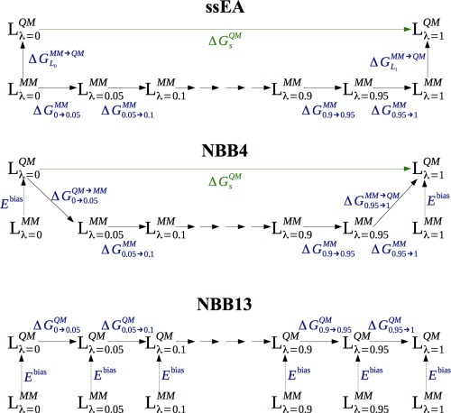
The various thermodynamic cycles employed in the ssEA, NBB4, and NBB13 methods to calculate binding free energies at the QM level. The cycles apply for the ligand simulated both with and without the host, giving either $\Delta G_{\text{bound}}^{\text{QM}}$ or $\Delta G_{\text{free}}^{\text{QM}}$ in eq. (2) (indicated by $\Delta G_s^{\text{QM}}$ in the figures). [Color figure can be viewed in the online issue, which is available at wileyonlinelibrary.com.]

Essex and coworkers have addressed this problem by considering only the electronic polarisation energy, which seems to give converged single‐step MM→QM/MM energies calculated by exponential averaging (ssEA; i.e., using the Zwanzig free‐energy perturbation approach;37 Fig. 1a) with ∼24,000 QM calculations for flexible ligands bound to cyclooxygenase‐2, as well as for small molecules in water solution, in both cases with only the ligand treated by QM.23, 28 However, they have also obtained converged QM/MM solvation free energies for small phenol analogues, including 200 water molecules in the QM calculations, considering interaction energies with only 1080 QM calculations.27 By performing full QM simulations, they have also shown that interaction energies (in contrast to total QM energies) give converged and consistent free energies for the MM→QM perturbation.38

König et al. instead reweighted the MM snapshots with QM energies, using the non‐Boltzmann Bennett acceptance ratio method (NBB; Fig. 1b).22 With this approach, they have obtained converged QM/MM hydration free energies using 4000–60,000 QM calculations, treating only the ligand by QM.29, 30

On the other hand, Mulholland and coworkers used full QM/MM Monte Carlo simulations, but employed the Metropolis–Hastings approach to reduce the number of QM calculations required.26 They have studied the relative hydration energy of water and methanol, as well as the binding of water molecules to neuraminidase, treating only the ligand by QM.24, 39 Still, the approach is very demanding, requiring 1.2–1.6·10⁵ QM calculations. However, recently Skylaris and coworkers have used a similar approach to calculate hydration free energies with full QM calculations, using QM/MM structures obtained by hybrid Monte Carlo simulation from MD simulations as an intermediate stepping stone.31 They obtained converged relative solvation energies by only 6000 QM calculations for each state.

We have employed both the ssEA and NBB approaches to calculate the relative binding affinities of nine cyclic carboxylic acids to the octa‐acid deep‐cavity host molecule (Figs. 2 and 3a) and for two synthetic disaccharides binding to galectin‐3, using the full host, all protein groups, and water molecules within 6 Å of the ligand in the QM calculations (287–312 atoms for the host–guest system and 744–748 atoms for galectin‐3) and dispersion‐corrected density‐functional theory with large basis sets (quadruple or triple zeta quality, respectively).13, 25 Unfortunately, it was not possible to obtain converged MM→QM/MM free energies for either system using 3600 QM calculations for each transformation.

Figure 2.

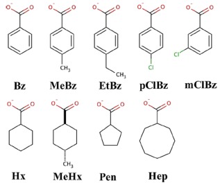
Guest molecules for the estimation of binding free energies to a truncated octa‐acid host. [Color figure can be viewed in the online issue, which is available at wileyonlinelibrary.com.]

Figure 3.

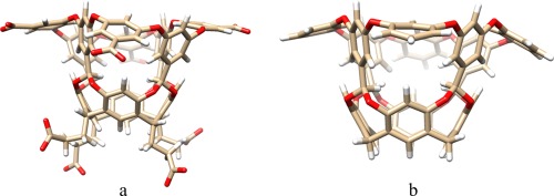
Structure of the full octa‐acid host (a) and the neutralized host, NOA without the propionate and carboxylate groups (b).

The full advantage of using QM calculations is not obtained until both the ligand and at least the closest groups of the receptor (4.5–6 Å40, 41, 42) are included in the QM calculations. So far, no converged QM/MM binding affinities have been obtained with such an approach, owing to the use of too demanding QM methods.13, 25 Therefore, we in this article turn to the cheaper (but more approximate) SQM methods and study what is needed to obtain converged MM→QM/MM free energies for the octa‐acid host–guest system. The emphasis is on convergence and what method gives the best convergence (we compare different variants of the ssEA and NBB methods), not on reproducing experimental data. We show that 720,000 QM calculations per transformation are required to converge the MM→QM free energies to within 1 kJ/mol.

Methods

Simulated system

In this article, we study the binding of nine cyclic carboxylate ligands to the octa‐acid host, using experimental data from the SAMPL4 challenge.43, 44 The ligands are shown in Figure 2 and the octa‐acid host in Figure 3a. Starting structures for the calculations were taken from our previous study of this system.13 To reduce the size and the large negative charge of the host and reduce its flexibility, we deleted the four propionate groups and also the four carboxylate groups on the rim of the ring system, giving rise to a neutral cavitand (NOA) with 144 atoms, shown in Figure 3b. We will show below that this truncation has only a minor effect on relative binding affinities estimated at the MM level, but it improves the convergence of the FES calculations.

The general Amber force field45 was used for both the NOA host and the ligands,13 and the TIP3P force field was used for water molecules.46 Restrained electrostatic potential (RESP) charges47 for the ligands were taken from our previous study13 and those of NOA were estimated in the same way: The host was optimized at the AM1 level48 and the electrostatic potential was calculated at the Hartree–Fock/6‐31G* level at points sampled around the molecule according to the Merz–Kollman scheme,49 albeit at a higher‐than‐default density (10 layers with 17 points per unit area, giving ∼2000 points per atom), using the Gaussian 09 software.50 The charges were then fitted to these potentials using the antechamber program in the Amber 14 suite.51 It was ensured that all symmetry‐equivalent atoms had the same charges (giving only 16 unique charges). The force field used for NOA is included in the Supporting Information, Table S1.

FES calculations at the MM level

All molecular dynamics (MD) simulations and FES calculations were performed with the Amber 13 (pre‐release) and 14 softwares.51 NOA and the ligands were solvated in a truncated octahedral box of water molecules, extending at least 9 Å from the solute using the leap program in the Amber suite, giving ∼4100 and ∼1800 atoms in total for the calculations with and without the host, respectively. Fifteen independent simulations were run for each ligand by solvating the systems in 15 different TIP3P water boxes of explicit water molecules and employing different random seeds for the starting velocities, to increase the difference between the independent simulations52). No counter‐ions were used in the calculations (implying that a neutralising plasma were added to the systems in the simulations), because we have previously shown that they only have a minor influence on the calculated free‐energy differences.13

The relative binding free energy between two ligands, L ₀ and L ₁ (ΔΔG _bind), was calculated for eight transformations: MeBz→Bz, EtBz→MeBz, pClBz→Bz, mClBz→Bz, Hx→Bz, MeHx→Hx, Hx→Pen, and Hep→Hx (the names of the ligands are defined in Fig. 2). The FES calculations were run with the pmemd module of Amber,51, 53 using the dual topology scheme with both ligands in the topology files. We employed 13 states with λ = 0.00, 0.05, 0.1, 0.2, …, 0.8, 0.9, 0.95, and 1.00, using a linear transformation of the potentials:

$$V_{\lambda }= \left(1\hspace{0.17em}–\hspace{0.17em}\lambda \right)V_0+\lambda V_1,$$ (1)

where V ₀ is the potential of the larger ligand and V ₁ is the potential of the smaller ligand. Electrostatic and van der Waals interactions were perturbed concomitantly, using soft‐core potentials for both types of interactions.54, 55 The soft‐core potentials were used only for atoms differing between the two guest molecules, that is, for the transformed CH₃ →H or Cl→H groups for the MeBz→Bz, EtBz→MeBz, pClBz→Bz, mClBz→Bz, and MeHx→Hx transformations, but for all atoms in the ring system for the Hx→Bz, Hx→Pen, and Hep→Hx transformations. Test calculations have shown that using soft‐core potentials for the whole guest molecule also for the smaller transformations does not change the results significantly.13 To make the calculations comparable between the two versions of Amber, we used the keyword tishake = 1 for the Amber 14 calculations.

For each λ value, we first performed 100 steps of minimisation, with the heavy atoms of the host and guest molecules restrained toward the starting structure with a force constant of 418.4 kJ/mol/Ų. This was followed by 20 ps constant‐volume equilibration with the same restraints and 2 ns constant‐pressure equilibration without any restraints. Finally, an 8 ns production simulation was run, during which structures were sampled every 2 ps. In the MD simulations, bonds involving hydrogen atoms were constrained with the SHAKE algorithm,56 allowing for a time‐step of 2 fs. In all simulations, the temperature was kept constant at 300 K using Langevin dynamics57 with a collision frequency of 2 ps⁻¹, and the pressure was kept constant at 1 atm using a weak‐coupling isotropic algorithm58 with a relaxation time of 1 ps. Long‐range electrostatics were handled by particle‐mesh Ewald (PME) summation59 with a fourth‐order B spline interpolation and a tolerance of 10⁻⁵. The cut‐off for Lennard–Jones interactions was set to 8 Å.

The relative binding free energies were estimated using a thermodynamic cycle that relates ΔΔG _bind to the free energy of alchemically transforming L ₀ into L ₁ when they are either bound to the host, ΔG _bound, or are free in solution, ΔG _free 60

$$\Delta \Delta G_{\text{bind}}= \Delta G_{\text{bind}}\left(L_1\right)\hspace{0.17em}-\hspace{0.17em}\Delta G_{\text{bind}}\left(L_0\right) = \Delta G_{\text{bound}}\hspace{0.17em}-\hspace{0.17em}\Delta G_{\text{free}}$$ (2)

ΔG _bound and ΔG _free can be estimated by the Bennett acceptance‐ratio method61, 62 (BAR). In this approach, an MD simulation is run for each λ, with the potential in eq. (1). For each pair of neighboring λ values, A and B, the free energy difference between the two states is estimated from

$$\Delta G^{A\to B}=RT\left(\text{ln}\frac{{〈f\left(V_A-V_B+C\right)〉}_B}{{〈f\left(V_B-V_A-C\right)〉}_A}\right)+C$$ (3)

where f(x) = (1 + exp(x/RT))⁻¹ is the Fermi function, R is the gas constant, T is the temperature (which was 300 K throughout this article), and C is a constant [if the number of samples are different in the two simulations, n _A ≠ n _B, a correction factor ln(n _A/n _B) should be added to the right‐hand side of eq. (3)]. An iterative procedure is applied to find a value of C that makes the first term of the right‐hand side of eq. (3) vanish. Free energies were also calculated by multi‐state BAR (MBAR),63 thermodynamic integration,64 and exponential averaging,37 using the pymbar software.63 Presented results were obtained with MBAR.

SQM calculations

SQM single‐point calculations were run on each of the MM snapshots, both for the simulations with and without NOA. For these calculations, water molecules were wrapped back into the original periodic box, centred on the ligand with the ptraj module. In the SQM calculations, the 48 water molecules closest to the ligand were included in the calculations without NOA, whereas the 19 water molecules closest to the C atom in the carboxylate group were included for the calculations with the ligand in NOA (in total 158–167 or 215–224 atoms, respectively; Fig. 4). This represents all water molecules within ∼4.5 Å of the ligand and they were obtained in the same way as in our previous study.13

Figure 4.

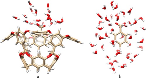
Example of structures used for the PM6‐DH2X calculations, including 19 or 48 water molecules for the calculations with (a) and without (b) NOA, respectively. [Color figure can be viewed in the online issue, which is available at wileyonlinelibrary.com.]

The PM6‐DH2X method65 was employed for the SQM calculations, that is, including dispersion, hydrogen‐bond, and halogen corrections,66, 67, 68 using the MOPAC software69 (this was the most accurate SQM method in this software when this investigation was started). The calculations employed the keyword Precise, to enhance the energy convergence criterion to 4.2·10⁻⁶ kJ/mol. For each snapshot, interaction energies were obtained by separate calculations for the complex, the guest, and the remainder (i.e., water molecules with or without NOA):13, 39

$$\Delta E_{\text{interact}}=E_{\text{complex}}\hspace{0.17em}-\hspace{0.17em}{E}_{\text{guest}}\hspace{0.17em}-\hspace{0.17em}{E}_{\text{remainder}}$$ (4)

MM→QM free energies

Several different methods were tested to calculate the MM→QM free energies. First, the QM interaction energies were used directly to calculate binding free energies for all λ values with the MBAR approach, that is, ignoring the fact that the MD simulations were not performed at the QM level. This will be called the QM‐MBAR approach.

Second, we employed ssEA calculations.13, 19, 20, 23, 27, 28 In these, we employ the thermodynamic cycle in Figure 1a, showing that ΔΔG _bind is first estimated at the MM level and then two single‐step FEP calculations are used to calculate the effect of changing the energy function from MM to QM, one for each of the two ligands:

$$\Delta G_s^{\text{QM}}=\Delta G_s^{\text{MM}}+\Delta G_{s,L_1}^{\text{MM}\to \text{QM}}-\Delta G_{s,L_0}^{\text{MM}\to \text{QM}}$$ (5)

where $\Delta G_s^{\text{MM}}$ is the free energy of the transformation at the MM level for either the bound or free states [subscript s; i.e., ΔG _bound or ΔG _free in eq. (2)], obtained by the standard MBAR approach, and the other two terms are correction terms for going from the MM potential to the QM potential. The latter corrections need to be evaluated only at the endpoints of the transformation, that is, for L ₀ in the λ = 0.00 snapshots and for L ₁ in the λ = 1.00 snapshots (for both the bound and free simulations). Each correction was evaluated either using exponential averaging (ssEA)37:

$$\Delta G_{s,{\mathrm{L}}_i}^{\text{MM}\to \text{QM}}=-RT\text{ln}{〈\text{exp}\left(-\left[E_{{\mathrm{L}}_i}^{\text{QM}}-E_{{\mathrm{L}}_i}^{\text{MM}}\right]/RT\right)〉}_{s,L_i}$$ (6)

or by using the cumulant expansion to the second order ( $\Delta G=\mu -\frac{{\sigma }^2}{2RT}$, where μ is the average and σ the standard deviation of the $E_{{\mathrm{L}}_i}^{\text{QM}}-E_{{\mathrm{L}}_i}^{\text{MM}}$ distribution; ssEAc),70, 71 which is exact if the energy differences follow a Gaussian distribution.

Third, we employed the NBB approach to reweight the snapshots.22 This method evaluates the free energy according to:

$$\Delta G^{\mathrm{A}\to \mathrm{B}}=RT\left(\frac{{〈f\left(E_{\mathrm{A}}^{\text{QM}}-E_{\mathrm{B}}^{\text{QM}}+C\right)\text{exp}\left(E_{\mathrm{B}}^{\text{bias}}/RT\right)〉}_{\mathrm{B}}{〈\text{exp}\left(E_{\mathrm{A}}^{\text{bias}}/RT\right)〉}_{\mathrm{A}}}{{〈f\left(E_{\mathrm{B}}^{\text{QM}}-E_{\mathrm{A}}^{\text{QM}}-C\right)\text{exp}\left(E_{\mathrm{A}}^{\text{bias}}/RT\right)〉}_{\mathrm{A}}{〈\text{exp}\left(E_{\mathrm{B}}^{\text{bias}}/RT\right)〉}_{\mathrm{B}}}\right)+C$$ (7)

where E ^bias = E ^MM–E ^QM. This bias is a correction for the fact that the simulations are performed at the MM level, but the energies are calculated at the QM level. The advantage with NBB is that the free energies are calculated with BAR, which has better convergence properties than EA, especially when the overlap is poor.62 The disadvantage is that at least twice as many QM calculations are needed, because BAR improves the convergence by employing the information from both a forward and backward calculation. Two different approaches to obtain the net binding free energies were used, as is illustrated in Figure 1. In the first, QM energies were calculated for all 13 λ values in the perturbation (Fig. 1c). This approach will be called NBB13 in the following. In the second approach, NBB was used only for the first two and last two λ values in the perturbation (Fig. 1b), as has been suggested by König and coworkers.29, 30 Thus, the net binding energy was obtained from

$$\Delta G_s^{\text{QM}}=\Delta G_s^{\text{QM}\left(\lambda =0\right)\to \text{MM}\left(\lambda =0.05\right)}+\Delta G_s^{\text{MM}\left(\lambda =0.05\to \lambda =0.95\right)}+\Delta G_s^{\text{MM}\left(\lambda =0.95\right)\to \text{QM}\left(\lambda =1\right)}$$ (8)

and the MM→QM energies were obtained from

$$\Delta G_s^{\text{QM}\left(\lambda =0\right)\to \text{MM}\left(\lambda =0.05\right)}=RT\left(\frac{{〈f\left(E_{\lambda =0}^{\text{QM}}-E_{\lambda =0.05}^{\text{MM}}+C\right)〉}_{s,\lambda =0.05}{〈\text{exp}(E_{\lambda =0}^{\text{bias}}/RT)〉}_{s,\lambda =0}}{{〈f\left(E_{\lambda =0.05}^{\text{MM}}-E_{\lambda =0}^{\text{QM}}-C\right)\text{exp}\left(E_{\lambda =0}^{\text{bias}}/RT\right)〉}_{s,\lambda =0}}\right)+C,$$ (9)

because the MM(λ = 0.05)→QM(λ = 0) perturbation is based on the MM(λ = 0.05) simulations, which are not biased, whereas the reverse transformation (QM(λ = 0)→MM(λ = 0.05)) is based on the MM(λ = 0) simulations, rather than the correct QM(λ = 0) simulations. It can be seen that QM calculations are needed only for L ₀, but not for L ₁. A similar equation applies for $\Delta G_s^{\text{MM}\left(\lambda =0.95\right)\to \text{QM}\left(\lambda =1\right)}$ (for which QM calculations are needed for L ₁, but not for L ₀). This approach will be called NBB4.

All potential energies (E ^QM, E ^MM, and E ^bias) in eqs. (6), (7), and (9) [and also eqs. (10)–(12) below] were approximated with the corresponding interaction energies, calculated by eq. (4). Moreover, the QM potential energies in the equations were calculated either for the isolated QM system (x _QM; i.e., the isolated guest with 49 water molecules or the host–guest complex with 19 water molecules) or for the full system with a QM/MM approach:

$$E^{\text{QM}/\text{MM}}=E^{\text{QM}}\left(x_{\text{QM}}\right)-E^{\text{MM}}\left(x_{\text{QM}}\right)+E^{\text{MM}}\left(x_{\text{all}}\right)$$ (10)

For the ssEA method in eqs. (5) and (6), the two approaches give the same result, because the energy difference in the exponential in eq. (6) becomes in the QM/MM case

$$E_{L_i}^{\text{QM}/\text{MM}}\left(x_{\text{all}}\right)-E_{L_i}^{\text{MM}}\left(x_{\text{all}}\right)=E_{L_i}^{\text{QM}}\left(x_{\text{QM}}\right)-E_{L_i}^{\text{MM}}\left(x_{\text{QM}}\right)+E_{L_i}^{\text{MM}}\left(x_{\text{all}}\right)-E_{L_i}^{\text{MM}}\left(x_{\text{all}}\right)=E_{L_i}^{\text{QM}}\left(x_{\text{QM}}\right)-E_{L_i}^{\text{MM}}\left(x_{\text{QM}}\right)$$ (11)

which is the same as in eq. (6). However, for NBB4 $E_{\lambda =0}^{\text{bias}}=E_{\lambda =0}^{\text{MM}}\left(x_{\text{QM}}\right)-E_{\lambda =0}^{\text{QM}}\left(x_{\text{QM}}\right)$ remains the same according to eq. (11), but eq. (9) changes to

$$\Delta G_s^{\mathrm{Q}\mathrm{M}/\mathrm{M}\mathrm{M}\left(\lambda =0\right)\to \mathrm{M}\mathrm{M}\left(\lambda =0.05\right)}=RT\left(\frac{{〈f\left(E_{\lambda =0}^{\text{QM}/\text{MM}}-E_{\lambda =0.05}^{\text{MM}}+C\right)〉}_{s,\lambda =0.05}{〈\text{exp}\left(E_{\lambda =0}^{\text{bias}}/RT\right)〉}_{s,\lambda =0}}{{〈f\left(E_{\lambda =0.05}^{\text{MM}}-E_{\lambda =0}^{\text{QM}/\text{MM}}-C\right)\text{exp}\left(E_{\lambda =0}^{\text{bias}}/RT\right)〉}_{s,\lambda =0}}\right)+C$$ (12)

with E ^QM/MM calculated from eq. (10) and the $\Delta G_s^{\text{MM}\left(\lambda =0.05\to \lambda =0.95\right)}$ energy calculated with the full systems, periodic boundary conditions, and total energies.

Uncertainties, quality estimates, and overlap measures

Reported uncertainties are standard errors, that is, standard deviations divided by the square root of the number of samples, for example, the 15 sets of independent simulations. The uncertainties of the free‐energy estimates were obtained by nonparametric bootstrap sampling (using 1000 samples) of the potential‐energy differences in the BAR or NBB calculations.

The quality of the binding‐affinity estimates compared to experimental data was quantified using the mean absolute deviation (MAD), the root‐mean‐squared deviation (RMSD), the correlation coefficient (r ²), and the slope and intercept of the best correlation line. In addition, Kendall's rank correlation coefficient was calculated for the eight transformations explicitly simulated (τ _r). The uncertainties of the quality estimates were obtained by a parametric bootstrap (using 500 samples), assuming the estimates follow a Gaussian distribution with the mean equal to the estimate and the standard deviation equal to the reported uncertainty.

To estimate the convergence of the various perturbations, six different overlap measures were employed.72 We calculated the Bhattacharyya coefficient for the energy distribution overlap (Ω),73 the Wu & Kofke overlap measures of the energy probability distributions (K _AB) and their bias metrics (Π),74, 75 the weight of the maximum term in the exponential average (w _max),20 the difference of the forward and backward exponential average estimate (ΔΔG _EA), and the difference between the BAR and TI estimates (ΔΔG _TI, although this difference may also reflect the integration error in TI76).72 We used w _max also to estimate the convergence of the ssEA and NBB4 calculations. In the former case, w _max is the weight of the maximum term in the average in eq. (6). In the latter case, w _max was calculated for each of the three averages in eq. (9) after convergence of C and the largest of these three values is reported. However, calculated in this way and using the same data, w _max for ssEA and NBB4 is identical, because the latter is always dominated by the $(\text{exp}\left(E_{\lambda =0}^{\text{bias}}/RT\right))$ term in eq. (9), which is the same as in eq. (6).

Result and Discussion

Binding affinities at the MM level

In this article, we study the binding of nine carboxylate ligands to the octa‐acid (OA) host molecule, shown in Figures 2 and 3a. We calculate the relative binding energies of the ligands with FES methods and our goal is to obtain converged relative binding energies at the QM/MM level, without performing sampling at the QM/MM level, but including all groups within ∼4.5 Å of the ligand in the QM calculations (not only the ligand as in most previous studies23, 24, 28, 29, 30, 39). Our previous investigation of this system as well as the binding of two ligands to galectin‐3 failed to give converged QM/MM binding energies with 3600 QM calculations at the DFT level.13, 25 Therefore, we employ here the much faster SQM PM6‐DH2X method, so that we can perform enough QM calculations to ensure converged results. Moreover, we have removed the propionate and benzoate groups of the octa‐acid host (yielding NOA, shown in Fig. 3b), because our previous study showed that it was hard to obtain a proper sampling of the dihedral angles of the propionate groups within a typical simulation time (4 ns).13 Moreover, the large negative charge (−8) of the host molecule sometimes gave problems in the QM calculations.

To check that the truncation of the host does not affect the results significantly, we first calculated ΔΔG _bind for the NOA host at the MM level. From the results in Table 1, it can be seen that the calculations with NOA gave almost the same results as for the full octa‐acid host13: For five of the transformations, the two hosts gave results that agreed within 1 kJ/mol, whereas for the remaining three transformations (EtBz→MeBz, Hx→Bz, and Hep→Hx), the results differed by 2–3 kJ/mol. However, owing to the high precision of both calculations, the difference is statistically significant for all except two of the transformations (MeBz→Bz and Hx→Pen) at the 95% level.

Table 1.

Results for the eight perturbations (ΔΔG _bind in kJ/mol) obtained at the MM level (using MBAR) for the NOA host.

Transformation	OA Exp.44	NOA MM calc.	OA13 MM calc.	NOA SQM/MM
MeBz→Bz	9.0±0.5	15.71±0.02	15.94±0.05	2.0±1.3
EtBz→MeBz	1.7±0.5	3.28±0.02	1.02±0.08	3.8±1.0
pClBz→Bz	12.6±0.2	18.60±0.02	19.06±0.09	6.8±1.0
mClBz→Bz	6.4±0.3	6.81±0.03	6.11±0.12	4.5±1.0
Hx→Bz	7.9±0.4	15.60±0.05	13.14±0.32	0.0±1.1
MeHx→Hx	8.3±0.4	14.81±0.01	15.35±0.15	5.0±1.1
Hx→Pen	7.9±0.4	8.33±0.04	7.48±0.73	0.0±1.0
Hep→Hx	4.1±0.3	7.35±0.07	5.50±0.66	7.2±0.9
MAD		4.07±0.13	3.56±0.17	4.9±0.4
RMSD		4.95±0.14	4.61±0.16	5.4±0.4
r 2		0.79±0.03	0.84±0.04	0.00±0.03
slope		1.50±0.07	1.77±0.09	0.0±0.1
inter		0.41±0.60	−2.40±0.75	3.9±0.9
τr		1.00±0.00	1.00±0.00	1.0±0.2

For comparison, calculated (BAR)13 and experimental44 results obtained with the full octa‐acid (OA) host are also included. For both NOA and OA, the presented calculated results are the average and standard error over the 15 or 10 independent simulations. In the last column, the SQM/MM results for the NOA host, obtained with ssEAc and 15 independent calculations are included. The six last rows give quality measures describing how well the calculations reproduce the experimental data of OA in the first column: The mean absolute deviation (MAD in kJ/mol), the root‐mean‐squared deviation (RMSD in kJ/mol), the correlation coefficient, the slope and intercept of the best correlation line, and Kendall's ranking correlation coefficient for only the eight considered transformations (τ_r).

The results of the NOA calculations are appreciably more precise than the OA calculations (0.02–0.08, compared to 0.05–0.73 kJ/mol). This is partly owing to the longer simulations (8 ns vs. 4 ns) and the larger number of independent simulations (15 vs. 10). However, there are also clear indications that the NOA calculations are better converged than the previous calculations: The overlap measures in Table 2 show a perfect overlap for all the eight transformations with NOA with all Ω = 1.00, K _AB ≥ 1.03, $\Pi$ ≥ 2.5, w _max ≤ 0.03, ΔΔG _EA ≤ 0.08 kJ/mol, and ΔΔG _TI ≤ 0.06 kJ/mol (Ω goes from 0, no overlap to 1, perfect overlap73; K _AB goes from 0 – no overlap, via 1 – full overlap, to 2 – the first distribution is completely inside the second distribution74, 75; a negative Π indicates poor overlap74, 75; 1/w _max indicates how many snapshots contribute significantly to the EA estimate; ΔΔG _EA is the hysteresis in the forward and backward EA estimates; and ΔΔG _TI indicates the difference between the BAR and TI estimates). In fact, all free‐energy measures estimated by PYMBAR (TI, TI_cubic EA_forward, EA_backward, BAR, and MBAR) agree within 0.06–0.19 kJ/mol for the eight transformations, and the most accurate BAR and MBAR results agree within 0.05 kJ/mol, indicating extremely well‐converged results.

Table 2.

Overlap measures for the eight perturbations of NOA and OA, performed at the MM level, based on 60,000 (NOA) or 4000 (OA) snapshots. Each measure is the minimum (Ω, K _AB, and $\Pi$) or maximum (w _max, ΔΔG _EA, and ΔΔG _TI) value over the 26 λ values for the simulations with and without the host.

	Ω	K AB	Π	w max	ΔΔG EA	ΔΔG TI
NOA
MeBz→Bz	1.00	1.03	2.9	0.003	0.02	0.04
EtBz→MeBz	1.00	1.04	2.7	0.004	0.03	0.03
pClBz→Bz	1.00	1.03	2.9	0.002	0.02	0.04
mClBz→Bz	1.00	1.03	2.8	0.002	0.06	0.02
Hx→Bz	1.00	1.03	2.5	0.004	0.06	0.02
MeHx→Hx	1.00	1.03	2.8	0.017	0.05	0.01
Hx→Pen	1.00	1.04	2.5	0.026	0.08	0.04
Hep→Hx	1.00	1.04	2.5	0.009	0.05	0.06
OA
MeBz→Bz	0.99	1.01	2.3	0.010	0.20	0.13
EtBz→MeBz	1.00	1.02	2.1	0.024	0.23	0.03
pClBz→Bz	1.00	1.02	2.5	0.009	0.12	0.14
mClBz→Bz	0.99	1.02	2.2	0.019	0.24	0.02
Hx→Bz	0.99	1.00	1.2	0.106	0.94	0.21
MeHx→Hx	0.93	0.79	1.1	0.947	16.19	0.34
Hx→Pen	0.95	0.85	0.0	0.716	1.69	0.06
Hep→Hx	0.98	0.93	−0.1	0.377	6.42	0.03

The measures are the Bhattacharyya coefficient for the energy distribution overlap (Ω),73 the Wu & Kofke overlap measures of the energy probability distributions (K _AB) and their bias metrics (Π)74, 75 the weight of the maximum term in the EA (w _max),20 the difference of the forward and backward EA estimate (ΔΔG _EA in kJ/mol), and the difference between the BAR and TI estimates (ΔΔG _TI in kJ/mol). Values indicating poor overlap or bad convergence are marked in bold face (Ω < 0.7, K _AB < 0.7, $\Pi$ < 0.5, w _max > 0.2, ΔΔG _EA > 4 kJ/mol, or ΔΔG _TI > 1 kJ/mol).72, 74, 75

For our previous OA simulations13 (also listed in Table 2), the convergence was appreciably worse with Ω down to 0.93, K _AB down to 0.79, Π down to −0.1, w _max up to 0.95, and ΔΔG _EA up to 16 kJ/mol, whereas ΔΔG _TI ≤ 0.3 kJ/mol was good. In particular, Hx→Pen and Hep→Hx transformation gave negative Π values and w _max > 0.38, which indicates that more λ values or longer simulations should have been used. This is also reflected by the larger standard error of these two estimates (0.7 kJ/mol). Moreover, the MeHx→Hx transformation gave w _max = 0.95 and ΔΔG _EA = 16 kJ/mol, which indicates that the overlap was poor also for this transformation. A large part of the improvement for NOA can be attributed to the longer simulations (60,000 snapshots instead of 4000). However, if we instead consider the worst values in the 15 independent simulations of NOA, each based on 4000 snapshots, NOA still gives converged results (Ω = 0.99, K _AB ≥ 0.93, Π ≥ 1.7, w _max ≤ 0.27, ΔΔG _EA ≤ 0.9 kJ/mol, and ΔΔG _TI ≤ 0.06 kJ/mol, although both w _max and ΔΔG _EA have increased by a factor of 6–17). This shows that the removal of the flexible propionate groups has strongly improved the sampling for the NOA host.

Affinities at the SQM level

Next, we tried to estimate binding affinities also at the SQM/MM level using 60,000 snapshots for each λ value (in practice, we first did the calculations on 4000 snapshots and based on those results, we decided how many independent simulations were needed to converge the results to a precision of 1 kJ/mol). As detailed in the Methods section, we employed several different approaches to calculate the MM→SQM free energies. First, we tried to use the full NBB13 approach with SQM calculations for all λ values (Fig. 1c). However, this is very demanding, requiring 60,000 · 13 · 2 · 5 = 7,800,000 QM calculations for each transformation (60,000 snapshots, 13 λ values, two sets of simulations, that is, with or without the host, calculations with both L ₀ and L ₁, and three calculations for each geometry to get interaction energies from eq. (4), but E _remainder is the same for the two ligands). Moreover, the calculations gave many numerical problems and highly uncertain results. The reason for this is partly that the MM calculations employ soft‐core potentials, which increase the difference between QM and MM and therefore deteriorates the convergence of the MM→QM perturbation. Therefore, this approach was only attempted for the MeBz→Bz transformation and for 4000 snapshots, giving $\Delta \Delta G_{\text{bind}}^{\text{NBB}13}$ = 29 ± 14 kJ/mol.

We also tried to calculate the binding free energies directly with MBAR calculations based on the QM results (QM‐MBAR; using the same data as NBB13), ignoring the fact that the snapshots were obtained with MD simulations at the MM, rather than the QM level.25 However, the results based on only 4000 snapshots for the MeBz→Bz transformation was poor (23.9 ± 0.1 kJ/mol), with large differences between estimates obtained with different methods (BAR, TI, and EA) and many overlap estimates indicating poor overlap, for example, Π down to −2.0, w _max up to 1.0, and ΔΔG _EA up to 949 kJ/mol. Therefore, this approach was not further pursued.

Instead, we tested the NBB4 approach suggested by König and coworkers.29, 30 In this approach, NBB is used to estimate the free energy of going from λ = 0.00 with QM to λ = 0.05 with MM (and similar between λ = 0.95 and 1.00), whereas the difference between λ = 0.05 and 0.95 is estimated at the MM level, as is illustrated in Figure 1b. NBB4 requires 60,000 · 4 · 2 · 3 = 1,440,000 QM calculations (i.e., only for λ = 0.00 and 0.05 with L ₀, and for λ = 0.95 and 1.00 with L ₁), which is 5.4 times fewer than with NBB13.

The NBB4 results are collected in Table 3. Two sets of results are presented: The first is for an NBB4 calculation including the concatenated results of all 60,000 snapshots with the standard error estimated by bootstrapping. The second is the average over the 15 individual independent calculations with 4000 snapshots in each and the standard error calculated from the standard deviation over the 15 sets. It can be seen that the uncertainty of the former approach is somewhat larger than for the latter, 2–7 vs. 2–3 kJ/mol. The opposite is normally observed, which indicates that the results strongly depend on a few snapshots, that is, that the calculations are still poorly converged. In most cases, the results of the two sets of calculations agree within the estimated statistical uncertainty, with differences of 1–8 kJ/mol. However, for the mClBz→Bz transformation, the difference is 20 kJ/mol, showing that the NBB4 estimates do not fully show the expected statistical behavior.

Table 3.

NBB4, ssEA, ssEAc, and ssPA results for the eight transformations (ΔΔG _bind or ΔΔG _MM→QM in kJ/mol).

Quantity	ΔΔG bind			ΔΔG MM→QM			ΔΔG bind	w max
Method	NBB4		ssEA	ssEAc		ssPA	ssEAc	ssEA
Averaging	all	15 indep	all	all	15 indep	all	15 indep	all
MeBz→Bz	−2.4±4.1	−1.1±2.9	−16.7±4.1	−13.8±1.0	−13.7±1.3	−11.6±0.16	3.1±1.3	0.76
EtBz→MeBz	−1.5±4.0	−4.5±3.2	−5.0±3.9	0.6±1.0	0.5±1.0	−2.8±0.17	4.4±1.0	0.87
pClBz→Bz	11.4±3.9	13.0±2.8	−10.7±4.0	−11.8±1.0	−11.8±1.0	−5.9±0.17	9.5±1.0	0.85
mClBz→Bz	31.9±7.2	9.6±3.8	11.9±4.9	−2.4±1.0	−2.4±1.0	−2.2±0.17	5.0±1.0	0.90
Hx→Bz	3.9±6.2	−3.7±2.2	−14.3±6.3	−15.5±1.0	−15.6±1.1	−29.9±0.17	3.5±1.1	0.92
MeHx→Hx	−1.4±5.1	5.6±2.9	−17.5±5.4	−10.0±0.9	−9.8±1.1	−3.8±0.16	6.8±1.1	0.96
Hx→Pen	−1.7±2.8	−2.4±3.3	−7.8±2.9	−8.4±1.0	−8.3±1.0	−4.5±0.16	0.5±1.0	0.55
Hep→Hx	17.4±2.2	11.1±2.8	9.3±2.2	−0.1±0.9	−0.2±0.9	−0.5±0.16	8.1±0.9	0.36

Results are shown for either all 60,000 snapshots in a single calculation with standard errors obtained with bootstrapping (all) or as the average over 15 independent simulations with 4000 snapshots each, obtaining standard errors from the standard deviation over these 15 results, divided by $\sqrt{15}$ (15 indep). In the last column, w _max is given for the ssEA–all calculation.

Therefore, we instead tried to estimate the MM→QM free energy by the ssEA approach. A direct application of ssEA [i.e., with the full exponential averaging in eq. (6)], gave an uncertainty similar to that for NBB4, 2–6 kJ/mol (third column in Table 3). Moreover, w _max = 0.36–0.96 (last column in Table 3), showing that the exponential average is dominated by one or a few terms (snapshots).

More stable results could be obtained by using a cumulant expansion to the second order70, 71 (which is equivalent of assuming a Gaussian distribution; ssEAc). With such an approach, the uncertainty was reduced to 0.9–1.0 kJ/mol for all eight transformations (based on calculations on all 60,000 snapshots and bootstrapped uncertainties; column four in Table 3). Closely similar results were obtained by averaging the results from the 15 independent simulations (with 4000 snapshots in each; column five in Table 3): The two approaches gave results that agreed within 0.2 kJ/mol and the uncertainties (estimated from the standard deviation over the 15 simulations) also agreed within a factor of 0.9–1.3. Moreover, the average standard errors for the individual calculations based on 4000 snapshots were 3.1–4.2 times larger than the standard errors for the calculations based on 60,000 snapshots, that is, close to $\sqrt{60000/4000}=\sqrt{15}$ = 3.9, following the expected $\sqrt{n}$ dependence of a normal distribution (in fact, we selected the final number of snapshots based on such an extrapolation). Figure 5 shows how the predictions converge and the precision improves with the number of snapshots. The results of the ssEA and ssEAc methods agree within 1–14 kJ/mol, which is inside the 95% confidence interval (dominated by the uncertainty of ssEA) for all transformations, except mClBz→Bz and Hep→Hx, indicating that the ssEA results are not fully well‐behaving. In Figure S1 in the Supporting Information, distribution and normal‐probability plots are given for three of the MM→QM perturbations. It can be seen that all E ^QM–E ^MM distributions are very close to normal, except in the low‐probability ends. The two first examples show typical results for simulations with and without the host, respectively, for which the distribution is Gaussian beyond 0.001 probability, whereas the last row shows the poorest results, for which deviations from Gaussian distribution start to emerge at 0.02 probability.

Figure 5.

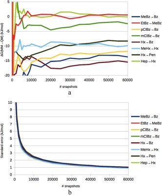
a) Convergence of the ssEAc predictions of ΔΔG _MM→QM with respect to the number of considered snapshots for the eight transformations. Pane b) shows the corresponding standard error of the calculations, based on 1000 bootstraps.

Three of the ligands are involved in more than one perturbation (Bz, MeBz, and Hx). Therefore, we have 2–4 estimates of ΔG _MM→QM for these for the simulations with or without the host, and these estimates are collected in Supporting Information Table S2. In most cases, the results of these calculations agree, for example, −90.1 to −90.8 kJ/mol for Bz with the host (average −90.7 ± 0.3 kJ/mol), in agreement with the estimated uncertainty of 0.4 kJ/mol for the individual estimates. However, in three cases, one of the simulations gives deviating results by 5–9 kJ/mol. This indicates that the ssEAc results still are somewhat sensitive to rare events in the simulations and occasionally the estimated precision is too high.

Finally, we also tried to estimate the MM→QM free energy with the pure average (ssPA), instead of the exponential average in the ssEA approach. This gave well‐converged results with a standard error of 0.2 kJ/mol, reflecting that a pure average has much better convergence properties than the exponential average (sixth column in Table 3). However, the pure average is an approximation to the true exponential average, an approximation that is valid only if the variation in the E ^QM–E ^MM energy differences is small, which is not the case. Therefore, the pure average converged to results that were different from those obtained with ssEAc. For the ΔΔG _MM→QM corrections in Table 3, the difference between the ssPA and ssEAc results for the various transformations was up to 14 kJ/mol (5 kJ/mol on average), a difference that is statistically significant for five of the transformations. However, ΔΔG _MM→QM is obtained as the difference of the results for the calculations with and without the NOA host, which each are the difference of the results obtained with L ₀ and L ₁ [eq. (2) and (5)]. For these four contributions to ΔΔG _MM→QM, the difference between ssPA and ssEAc was much larger, 59–237 kJ/mol. This clearly shows that pure averages cannot be used if you aim at an accuracy better than ∼10 kJ/mol, especially as there is no useful estimate of the true uncertainty of the approach.

The NBB and ssEA results discussed so far are not comparable, because the former are full ΔG _bind free energies, whereas the latter only includes the MM→QM free‐energy correction (ΔΔG _MM→QM in Table 3). Thus, to compare the results, we need to add $\Delta \Delta G_{\text{bind}}^{\text{MM}}$, obtained for the isolated QM system at the MM level. This is done in the penultimate column in Table 3. It can be seen that the NBB4 and ssEAc results agree within 1–9 kJ/mol (based on averages of the 15 independent simulations), which is reasonable, considering the quite large uncertainty of the NBB4 results.

All SQM results discussed up to this point have been based on calculations of the isolated QM system. More realistic energies can be obtained by a QM/MM approach. As discussed in the Methods section, QM and QM/MM energies give the same results for ssEA, so we easily reach a final result by adding the MM→QM ssEAc free‐energy corrections in Table 3 (column five) to the ΔΔG _bind free energies, obtained at the MM level for the full periodic system from the second column in Table 1, giving the results in last column of Table 1. These results differ slightly from the results in the penultimate column in Table 3, because the latter employ MM $\Delta \Delta G_{\text{bind}}^{\text{MM}}$ binding free energies obtained for only the QM system and using interaction energies instead of total potential energies (to make the results directly comparable with the NBB4 results in Table 3 which use the same MM $\Delta \Delta G_{\text{bind}}^{\text{MM}}$ free energies). The two results differ by up to 3.5 kJ/mol (1.5 kJ/mol on average), showing that already the small QM system gives reasonable $\Delta \Delta G_{\text{bind}}^{\text{MM}}$ free‐energy estimates.

From Figure 6, it can be seen that all MM→QM corrections are in the correct direction (assuming that NOA should give the same results as OA), that is, reducing the relative affinities, except in the EtBz→MeBz case, for which the MM→QM correction is close to zero. Unfortunately, the corrections are too large in six of the cases, giving too small relative binding affinities. Consequently, the SQM/MM results reproduce the experimental OA results appreciably worse than the MM results, as is shown in Table 1. For example, MAD increases to 4.9 ± 0.4 kJ/mol and r ² vanishes. Of course, this is somewhat disappointing after performing almost 6 million SQM calculations. However, this result is much better than previous attempts to obtain QM/MM FES binding free energies for the same system, which gave MADs of 17–26 kJ/mol and no convergence for the MM → QM perturbation.13 It is also much better than approaches based on optimized structures and energies calculated by dispersion‐corrected DFT methods or even CCSD(T) calculations, giving MADs of 8–37 kJ/mol.13, 14, 15 Moreover, our aim has been to find out what is required to converge the MM→QM/MM, not to reproduce the experimental results. Therefore, we have selected a rather cheap method, PM6‐D2HX, which is among the best available SQM methods, although it is appreciably worse than dispersion‐corrected DFT methods.77

Figure 6.

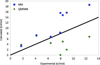
Comparison of the MM and SQM/MM (ssEAc) results for NOA, compared to the experimental relative affinities44 for the eight considered transformations. The black line shows the perfect correlation. [Color figure can be viewed in the online issue, which is available at wileyonlinelibrary.com.]

Thus, at least for this data, ssEAc with the cumulant expansion gave a lower uncertainty than NBB4. A possible reason for this is again the use of soft‐core potentials in the MM calculations, which increases the difference between QM and MM: In the ssEA approach, only the λ = 0.00 and 1.00 states are considered, for which the soft‐core potentials are not active. However, NBB4 considers also the λ = 0.05 and 0.95 states, for which the soft‐core is active. The ssEA approach also has the advantage of using only 60,000 · 2 · 2 · 3 = 720,000 QM calculations (i.e., only for L ₀ at λ = 0.00 and L ₁ at λ = 1.00), that is, half as many as for NBB4. Moreover, the reweighting in NBB is often badly conditioned, essentially picking out a single energy (snapshot) in the second average in the nominator of eq. (9). In fact, w _max calculated for this method is exactly the same as for ssEA (shown in the last column in Table 3), that is, 0.36–0.96, indicating that the estimated free energies are completely dominated by one or a few QM energies (and that the use of numerous QM calculations is only a way of finding these values). This explains the rather poor convergence of both these methods. On the other hand, with the cumulant expansion, all QM values are used to estimate the average and standard deviation of the Gaussian distribution (but both values are still somewhat dominated by a few values).

All results in Table 3 were obtained using interaction energies [eq. (4)] rather than total energies. This has the advantage of making the E ^QM–E ^MM energy difference smaller and less varying by ignoring the difference in the two energy functions for the internal interactions within the ligand or the host. On the other hand, this is an approximation. At the MM level, it is a good approximation: For seven of the perturbations, ΔΔG _bind calculated with interaction energies (and without periodicity and Ewald summation) reproduce the results in Table 1 (based on total energies) within 0.6 kJ/mol (MAD 0.3 kJ/mol). However, for the Hx→Bz perturbation, the difference is slightly larger, 2.7 kJ/mol. On the other hand, using total energies for the MM→QM perturbation increases the variation in E ^QM–E ^MM by a factor of ∼2, making the convergence much worse. As a consequence, ΔΔG _MM→QM estimated by ssEAc changes by 1–12 kJ/mol (5 kJ/mol on average; pure averages change by 1–4 kJ/mol) and the bootstrapped precision estimates become very large, illustrating that these results are far from converged. This shows that interaction energies strongly improve the convergence of the MM→QM perturbations, in agreement with other studies.38, 78

Conclusions

In this article, we have studied what is needed to obtain converged QM/MM relative binding free energies, performing sampling only at the MM level and including a significant surrounding of the ligand in the QM calculations (158–224 atoms). Previous studies with such an approach have given poorly converged results both for a host–guest system and a full protein, probably owing to the use of too few QM calculations (3600 per transformation).13, 25

Therefore, we have here employed a system for which we can perform many more QM calculations: First, we used the octa‐acid host–guest system, which is smaller and simpler than a protein. Second, we removed all eight carboxylate groups on the host molecule to further reduce the size of the system, to remove possible problems of the extensive net charge of the host, and to reduce the flexibility of the host and therefore improve the sampling of the phase space. Third, we employed the SQM PM6‐DH2X method, which is computationally much cheaper than the DFT methods we have used in our previous studies. On the other hand, this means that we cannot strictly compare to any experimental results and that we use a QM method with an appreciably lower accuracy than dispersion‐corrected DFT methods.77

We first showed that the truncation of the host gave rather restricted changes in relative binding free energies, as estimated at the MM level, up to 3 kJ/mol. Moreover, the new calculations were much more precise than those based on the full OA host, with a precision of 0.02–0.08 kJ/mol. This was partly an effect of the longer simulations (120 ns per λ value), but there were also clear indications that the sampling has been improved. In particular, our overlap measures clearly showed that the simulations were perfectly converged, in variance to the original simulations.

Next, we tested six different methods to calculate relative binding free energies at the QM level. We showed that approaches based on QM calculations for all 13 λ values (both NBB13 and QM‐MBAR) were very expensive and gave poorly converged results. On the other hand, NBB4 and ssEA gave promising results, although a full convergence could not be obtained even with 1,440,000 or 720,000 QM calculations per transformation, respectively. Instead, the results indicated that 3–50 times more QM calculations are needed for convergence and this is most likely an underestimate owing to the bad conditioning of these methods (they strongly depend on one or very few of the calculated values).

However, the ssEAc approach with the cumulant expansion gave nicely converged results with a standard error of 1 kJ/mol using 720,000 QM calculations per λ transformation for all eight studied relative free energies. Moreover, it showed the expected square‐root dependence of the standard error with respect to the number of calculations. It also required half as many QM calculations as the NBB4 approach. Pure averages for the MM→QM perturbation also gave converged free energies, but the results differed from those obtained by ssEAc by up to 14 kJ/mol, because this is only an approximate method that strictly should not work when the variation in the MM–QM energy differences is large.

The required number of QM calculations is of a comparable magnitude to what has been used in previous QM/MM‐FES studies by Mulholland and coworkers,24, 26 especially as they included only a single rigid water molecule in the QM system. König et al. also had to perform 20,000–60,000 QM calculations to obtain an uncertainty of up to 2 kJ/mol, again including only a small solute in the QM system.30 However, Skylaris et al. have included the solute and 200 water molecules in the QM calculations, calculating the free energies by ssEA, based on interaction energies.27 Still, they claim to obtain converged relative solvation free energies (within 4 kJ/mol) with only 1080 QM calculations per transformation. The reason for this seems to be a smaller difference between the QM and MM potentials (although they use the same GAFF/TIP3P MM method as we do): They report a range for the E ^QM–E ^MM energy difference of ∼55 kJ/mol, whereas it is almost four times larger in our study, 181–211 kJ/mol. The convergence of FES strongly depend on this range—in the well‐converged FES calculations at the MM level (with 13 λ values), the range is typically ∼10 kJ/mol with a maximum of 38 kJ/mol. The reason for the lower range in the studies by Skylaris et al. is probably that they study only simple and rigid phenol derivatives. In a recent study with more flexible (but smaller) molecules, they employed more QM calculations and included also an intermediate QM/MM step to improve the convergence with only the solute in the QM, performing QM/MM MD simulations.31 Finally, it should also be noted that König et al. have in two studies suggested that NBB4 gives better convergence than ssEA (for absolute solvation free energies).29, 30 However, they did not employ the cumulant expansion for ssEA, which strongly improves the convergence in this study. In fact, very recently they published a study of hydration free energies of 20 organic molecules, in which they come to conclusions very similar to ours:78 With a cumulant expansion, they obtain a slightly better convergence of the QM/MM free energies with ssEAc than with NBB4, both analytically and in practice. This shows that our conclusions apply also to other types of systems.

Consequently, we recommend the ssEAc method to obtain converged QM/MM binding free energies. Still, our results show that a very large number of QM calculations are needed to obtain strict QM/MM FES binding free energies, 720,000 per perturbation. This provides a useful guide for future studies of QM/MM binding free energies: The QM method and the size of the QM system have to be selected to allow for such an amount of QM calculations. Moreover, it provides a firm basis for comparison with alternative methods. It has recently been shown that reasonable binding free energies can be obtained with single structures optimized with dispersion‐corrected DFT methods for host–guest systems;77, 79 in fact, relative energies for ligands binding to the same host were reproduced with a MAD of 5 kJ/mol. Such an approach requires only a few hundred QM energy calculations. Unfortunately, the approach worked appreciably worse for the OA system, with MADs of 5–10 kJ/mol, probably owing to the larger flexibility and the high charge of this host.13, 14 Alternatively, full QM/MM MD simulation could be performed; 720,000 QM calculations correspond to 0.36–1.4 ns simulations, depending on the time step, which may give converged FES results. Thus, it might be better to spend the QM calculations on true FES calculations with sampling at the QM/MM level instead. This is currently investigated in our group.

Supporting information

Additional Supporting Information are found in the online version of this article.

Supporting Information

How to cite this article: Olsson M. A., Söderhjelm P., Ryde. U. J. Comput. Chem. 2016, 37, 1589–1600. DOI: 10.1002/jcc.24375

References

- 1. Gohlke H., Klebe G., Angew. Chem. Int. Ed. Engl. 2002, 41, 2644. [DOI] [PubMed] [Google Scholar]
- 2. Wereszczynski J., McCammon J. A., Q. Rev. Biophys. 2012, 45, 1. [DOI] [PMC free article] [PubMed] [Google Scholar]
- 3. Hansen N., van Gunsteren W. F., J. Chem. Theory Comput. 2014, 10, 2632. [DOI] [PubMed] [Google Scholar]
- 4. Raha K., Peters M. B., Wang B., Yu N., Wollacott A. M., Westerhoff L. M., Merz K. M., Drug Discov. Today 2007, 12, 725. [DOI] [PubMed] [Google Scholar]
- 5. Söderhjelm P., Genheden S., Ryde U., In Protein‐Ligand Interactions; Gohlke H., Ed.; Wiley‐VCH Verlag: Weinheim, Vol. 53, 2012; pp. 121–143. [Google Scholar]
- 6. Ryde U., Söderhjelm P., Chem. Rev. DOI: 10.1021/acs.chemrev.5b00630. [DOI] [PubMed] [Google Scholar]
- 7. Raha K., Merz K. M., J. Am. Chem. Soc. 2004, 126, 1020. [DOI] [PubMed] [Google Scholar]
- 8. Cho A. T., Guallar V., Berne B. J., Friesner R., J. Comput. Chem. 2005, 26, 915. [DOI] [PMC free article] [PubMed] [Google Scholar]
- 9. Gräter F., Schwarzl S. M., Dejaegere A., Fischer S., Smith J. C., J. Phys. Chem. B 2005, 109, 10474. [DOI] [PubMed] [Google Scholar]
- 10. Fanfrlík J., Bronowska A. K., Rezác J., Prenosil O., Konvalinka J., Hobza P., J. Phys. Chem. B 2010, 114, 12666. [DOI] [PubMed] [Google Scholar]
- 11. Söderhjelm P., Kongsted J., Ryde U., J. Chem. Theory Comput. 2010, 6, 1726. [DOI] [PubMed] [Google Scholar]
- 12. Mikulskis P., Genheden S., Wichmann K., Ryde U., J. Comput. Chem. 2012, 33, 1179. [DOI] [PubMed] [Google Scholar]
- 13. Mikulskis P., Cioloboc D., Andrejic M., Khare S., Brorsson J., Genheden S., Mata R. A., Söderhjelm P., Ryde U., J. Comput. Aided Mol. Des. 2014, 28, 375. [DOI] [PubMed] [Google Scholar]
- 14. Sure R., Antony J., Grimme S., J. Phys. Chem. B 2014, 118, 3431. [DOI] [PubMed] [Google Scholar]
- 15. Andrejic M., Ryde U., Mata R., Söderhjelm P., Chem. Phys. Chem. 2014, 15, 3270. [DOI] [PubMed] [Google Scholar]
- 16. Reddy M. R., Erion M. D., J. Am. Chem. Soc. 2007, 129, 9296. [DOI] [PubMed] [Google Scholar]
- 17. Rathore R. S., Reddy R. N., Kondapi A. K., Reddanna P., Reddy M. R., Theor. Chem. Acc. 2012, 131, 1096. [Google Scholar]
- 18. Swiderek K., Marti S., Moliner V., Phys. Chem. Chem. Phys. 2012, 14, 12614. [DOI] [PubMed] [Google Scholar]
- 19. Luzhkov V., Warshel A., J. Comput. Chem. 1992, 13, 199. [Google Scholar]
- 20. Rod T. H., Ryde U., Phys. Rev. Lett. 2005, 94, 138302. [DOI] [PubMed] [Google Scholar]
- 21. Duarte F., Amrein B. A., Blaha‐Nelson D., Kamerlin S. C. L., Biochim. Biophys. Acta 2015, 1850, 954. [DOI] [PMC free article] [PubMed] [Google Scholar]
- 22. König G., Boresch S., J. Comput. Chem. 2011, 32, 1082. [DOI] [PubMed] [Google Scholar]
- 23. Beierlein F. R., Michel J., Essex J. W., J. Phys. Chem. B 2011, 115, 4911. [DOI] [PubMed] [Google Scholar]
- 24. Woods C. J., Shaw K. E., Mulholland A. J., J. Phys. Chem. B 2015, 119, 997. [DOI] [PubMed] [Google Scholar]
- 25. Genheden S., Söderhjelm P., Ryde U., J. Comput. Chem. 2015, 36, 2114. [DOI] [PubMed] [Google Scholar]
- 26. Woods C. J., Manby F. R., Mulholland A. J., J. Chem. Phys. 2008, 128, 014109. [DOI] [PubMed] [Google Scholar]
- 27. Fox S. J., Pittock C., Tautermann C. S., Fox T., Christ C., Malcolm N. O. J., Essex J. W., Skylaris C. K., J. Phys. Chem. B 2013, 117, 9478. [DOI] [PubMed] [Google Scholar]
- 28. Genheden S., Cabedo Martinez A. I., Criddle M. P., Essex J. W., J. Comput. Aided Mol. Des. 2014, 28, 187. [DOI] [PubMed] [Google Scholar]
- 29. König G., Pickard F. C., Mei Y., Brooks B. R., J. Comput. Aided Mol. Des 2014, 28, 245. [DOI] [PMC free article] [PubMed] [Google Scholar]
- 30. König G., Hudson P. S., Boresch S., Woodcock H. L., J. Chem. Theory Comput. 2014, 10, 1406. [DOI] [PMC free article] [PubMed] [Google Scholar]
- 31. Sampson C., Fox T., Tautermann C. S., Woods C., Skylaris C. K. A., J. Phys. Chem. B 2015, 119, 7030. [DOI] [PubMed] [Google Scholar]
- 32. Hu H., Yang W., Annu. Rev. Phys. Chem. 2008, 59, 573. [DOI] [PMC free article] [PubMed] [Google Scholar]
- 33. Senn H. M., Thiel W., Angew. Chem. Int. Ed. 2009, 48, 1198. [DOI] [PubMed] [Google Scholar]
- 34. Heimdal J., Ryde U., Phys. Chem. Chem. Phys. 2012, 14, 12592. [DOI] [PubMed] [Google Scholar]
- 35. Strajbl M., Hong G., Warshel A., J. Phys. Chem. B 2002, 106, 13333. [Google Scholar]
- 36. Plotnikov N. V., Warshel A., J. Phys. Chem. B 2012, 116, 10342. [DOI] [PMC free article] [PubMed] [Google Scholar]
- 37. Zwanzig R. W., J. Chem. Phys. 1954, 22, 1420. [Google Scholar]
- 38. Cave‐Ayland C., Skylaris C. K., Essex J. W., J. Phys. B 2015, 119, 1017. [DOI] [PubMed] [Google Scholar]
- 39. Shaw K. E., Woods C. J., Mulholland A. J., J. Phys. Chem. Lett. 2010, 1, 219. [Google Scholar]
- 40. Hu L., Eliasson J., Heimdal J., Ryde U., J. Phys. Chem. A 2009, 113, 11793. [DOI] [PubMed] [Google Scholar]
- 41. Söderhjelm P., Ryde U., J. Phys. Chem. A 2009, 113, 617. [DOI] [PubMed] [Google Scholar]
- 42. Hu L., Söderhjelm P., Ryde U., J. Chem. Theory Comput. 2013, 9, 640. [DOI] [PubMed] [Google Scholar]
- 43. Muddana H. S., Fenley A. T., Mobley D. L., Gilson M. K., J. Comput. Aided Mol. Des. 2014, 28, 305. [DOI] [PMC free article] [PubMed] [Google Scholar]
- 44. Gibb C. L. D., Gibb B., J. Comput. Aided Mol. Des. 2014, 28, 319. [DOI] [PMC free article] [PubMed] [Google Scholar]
- 45. Wang J. M., Wolf R. M., Caldwell K. W., Kollman P. A., Case D. A., J. Comput. Chem. 2004, 25, 1157. [DOI] [PubMed] [Google Scholar]
- 46. Jorgensen W. L., Chandrasekhar J., Madura J. D., Impey R. W., Klein M. L., J. Chem. Phys. 1983, 79, 926. [Google Scholar]
- 47. Bayly C. I., Cieplak P., Cornell W. D., Kollman P. A., J. Phys. Chem. 1993, 97, 10269. [Google Scholar]
- 48. Dewar M. J. S., Zoebisch E. G., Healy E. F., Stewart J. J. P., J. Am. Chem. Soc. 1985, 107, 3902. [Google Scholar]
- 49. Besler B. H., Merz K. M., Kollman P. A. J., Comput. Chem. 1990, 11, 431. [Google Scholar]
- 50. Frisch M. J., Trucks G. W., Schlegel H. B., Scuseria G. E., Robb M. A., Cheeseman J. R., Scalmani G., Barone V., Mennucci B., Petersson G. A., Nakatsuji H., Caricato M., Li X., Hratchian H. P., Izmaylov A. F., Bloino J., Zheng G., Sonnenberg J. L., Hada M., Ehara M., Toyota K., Fukuda R., Hasegawa J., Ishida M., Nakajima T., Honda Y., Kitao O., Nakai H., Vreven T., J. A. Jr Montgomery, ., Peralta J. E., Ogliaro F., Bearpark M., Heyd J. J., Brothers E., Kudin K. N., Staroverov V. N., Kobayashi R., Normand J., Raghavachari K., Rendell A., Burant J. C., Iyengar S. S., Tomasi J., Cossi M., Rega N., Millam J. M., Klene M., Knox J. E., Cross J. B., Bakken V., Adamo C., Jaramillo J., Gomperts R., Stratmann R. E., Yazyev O., Austin A. J., Cammi R., Pomelli C., Ochterski J. W., Martin R. L., Morokuma K., Zakrzewski V. G., Voth G. A., Salvador P., Dannenberg J. J., Dapprich S., Daniels A. D., Farkas Ö., Foresman J. B., Ortiz J. V., Cioslowski J., Fox D. J., Gaussian 09, revision A. 02; Gaussian, Inc: Wallingford, CT, 2009. [Google Scholar]
- 51. Case D. A., Berryman J. T., Betz R. M., Cerutti D. S., Cheatham T. E., III, Darden T. A., Duke R. E., Giese T. J., Gohlke H., Goetz A. W., Homeyer N., Izadi S., Janowski P., Kaus J., Kovalenko A., Lee T. S., LeGrand S., Li P., Luchko T., Luo R., Madej B., Merz K. M., Monard G., Needham P., Nguyen H., Nguyen H. T., Omelyan I., Onufriev A., Roe D. R., Roitberg A., Salomon‐Ferrer R., Simmerling C. L., Smith W., Swails J., Walker R. C., Wang J., Wolf R. M., Wu X., York D. M., Kollman P. A., AMBER; University of California: San Francisco, 2015. [Google Scholar]
- 52. Genheden S., Ryde U., J. Comput. Chem. 2011, 32, 187. [DOI] [PubMed] [Google Scholar]
- 53. Kaus J. W., Pierce L. T., Walker R. C., McCammon J. A., J. Chem. Theory Comput. 2013, 9, 4131. [DOI] [PMC free article] [PubMed] [Google Scholar]
- 54. Steinbrecher T., Mobley D. L., Case D. A., J. Chem. Phys. 2007, 127, 214108. [DOI] [PubMed] [Google Scholar]
- 55. Steinbrecher T., Joung I., Case D. A., J. Comput. Chem. 2011, 32, 3253. [DOI] [PMC free article] [PubMed] [Google Scholar]
- 56. Ryckaert J. P., Ciccotti G., Berendsen H. J. C., J. Comput. Phys. 1977, 23, 327. [Google Scholar]
- 57. Wu X., Brooks B. R., Phys. Lett. 2003, 381, 512. [Google Scholar]
- 58. Berendsen H. J. C., Postma J. P. M., van Gunsteren W. F., Dinola A., Haak J. R., J Chem. Phys. 1984, 81, 3684. [Google Scholar]
- 59. Darden T., York D., Pedersen L., J. Chem. Phys. 1993, 98, 10089. [Google Scholar]
- 60. Tembe B. L., McCammon J. A., Comput. Chem. 1984, 8, 281. [Google Scholar]
- 61. Bennett C. H., J. Comput. Phys. 1976, 22, 245. [Google Scholar]
- 62. Shirts M. R., Pande V. S., J. Chem. Phys. 2005, 122, 144107. [DOI] [PubMed] [Google Scholar]
- 63. Shirts M. R., Chodera J. D., J. Chem. Phys. 2008, 129, 124105. [DOI] [PMC free article] [PubMed] [Google Scholar]
- 64. Kirkwood J. G., J. Chem. Phys. 1935, 3, 300. [Google Scholar]
- 65. Stewart J. J. P., J. Mol. Model. 2007, 13, 1173. [DOI] [PMC free article] [PubMed] [Google Scholar]
- 66. Korth M., Pitonák M., Rezác J., Hobza P., J. Chem. Theory Comput. 2010, 6, 344. [DOI] [PubMed] [Google Scholar]
- 67. Rezác J., Fanfrlik J., Salahub D., Hobza P., J. Chem. Theory Comput. 2009, 5, 1749. [DOI] [PubMed] [Google Scholar]
- 68. Rezác J., Hobza P., Chem. Phys. Lett. 2011, 506, 266. [Google Scholar]
- 69. Stewart J. J. P., MOPAC2012, Stewart Computational Chemistry; Colorado Springs: CO. [Google Scholar]
- 70. Hummer G., Szabo A., J. Chem. Phys. 1996, 105, 2004. [Google Scholar]
- 71. Kästner J., Senn H. M., Thiel S., Otte N., Thiel W., J. Chem. Theory Comput. 2006, 2, 452. [DOI] [PubMed] [Google Scholar]
- 72. Mikulskis P., Genheden S., Ryde U., J. Chem. Inf. Model. 2014, 54, 2794. [DOI] [PubMed] [Google Scholar]
- 73. Bhattacharyya A., Bull. Cal. Math. Soc. 1943, 35, 99. [Google Scholar]
- 74. Wu D., Kofke D. A., J. Chem. Phys. 2005, 123, 054103. [DOI] [PubMed] [Google Scholar]
- 75. Pohorille A., Jarzynski A., Chipot C., J. Chem. Phys. B 2010, 114, 10235. [DOI] [PubMed] [Google Scholar]
- 76. Li H., Yang W., Chem. Phys. Lett. 2007, 440, 155. [Google Scholar]
- 77. Sure R., Grimme S., J. Chem. Theory Comput. 2015, 11, 3785. [DOI] [PubMed] [Google Scholar]
- 78. Jia X., Wang M., Shao Y., König G., Brooks B. R., Zhang J. Z. H., Mei Y., J. Chem. Theory Comput. 2016, 12, 499. [DOI] [PubMed] [Google Scholar]
- 79. Grimme S., Chem. Eur. J. 2012, 18, 9955. [DOI] [PubMed] [Google Scholar]
Associated Data
This section collects any data citations, data availability statements, or supplementary materials included in this article.
Supplementary Materials