Calibrating random forests for probability estimation

Abstract

Probabilities can be consistently estimated using random forests. It is, however, unclear how random forests should be updated to make predictions for other centers or at different time points. In this work, we present two approaches for updating random forests for probability estimation. The first method has been proposed by Elkan and may be used for updating any machine learning approach yielding consistent probabilities, so‐called probability machines. The second approach is a new strategy specifically developed for random forests. Using the terminal nodes, which represent conditional probabilities, the random forest is first translated to logistic regression models. These are, in turn, used for re‐calibration. The two updating strategies were compared in a simulation study and are illustrated with data from the German Stroke Study Collaboration. In most simulation scenarios, both methods led to similar improvements. In the simulation scenario in which the stricter assumptions of Elkan's method were not met, the logistic regression‐based re‐calibration approach for random forests outperformed Elkan's method. It also performed better on the stroke data than Elkan's method. The strength of Elkan's method is its general applicability to any probability machine. However, if the strict assumptions underlying this approach are not met, the logistic regression‐based approach is preferable for updating random forests for probability estimation. © 2016 The Authors. Statistics in Medicine Published by John Wiley & Sons Ltd.

1. Introduction

Accurate estimation of outcome probabilities for individuals is important in medical practice. Applications are, for example, diagnosis, decision on therapy, or prognosis. If a predictive model is applied in other centers or at different time points, it is necessary to assess its generalizability, that is, its ability to provide accurate predictions in a new sample of patients 1. Validation data may also be used to update the model, thus to improve its predictive performance in the new sample. Effective updating strategies are available for logistic regression, which is the standard approach for probability estimation. One such approach is re‐calibration. Here, the intercept of the logistic regression model is re‐estimated, while the other coefficients are kept unchanged 2. This means that we understand calibration as a way to correct too low or too high predicted probabilities 1, not to find a mapping from score vectors to probability vectors 3. To guarantee consistent probability estimates, the logistic regression model needs to be correctly specified. The correct model specification is, however, challenging in case of nonlinear effects, high‐dimensional data, and collinearity between independent variables. One approach to overcome these challenges is the use of nonparametric machine learning methods, such as random forests for probability estimation.

Random forests were introduced by Breiman for classification problems 4, and they are an extension of classification and regression trees (CART) 5. Advantages of the CART algorithm are its simple interpretation, implementation, and application. However, random forests are generally preferable over CART. For specific versions of random forests, it has been shown that the variance of random forests is smaller than the variance of a single tree 6. Random forests can also have a faster convergence rate than single CART 6. The convergence rate of random forests may even be faster than the standard minimax rate of nonparametric regression 7. Finally, and most importantly for probability estimation, random forests allow consistent estimation of individual probabilities 8, 9, while probability estimation trees generally yield biased estimates 10.

It is, however, unclear how random forests for probability estimation should be updated to another population or a more recent time period. One approach for updating probability estimates has been described by Elkan 11. This method can be applied to any probability machine, that is, any machine learning method yielding consistent individual probability estimates. The broad applicability of this approach comes at the cost of strict assumptions regarding the distribution of the covariates in the data sets used for model development and updating.

In this work, we propose a logistic regression‐based updating approach for random forests, which has weaker assumptions than Elkan's approach. A random forest is estimated first and next translated to logistic regression models. These estimates are then updated using re‐calibration for logistic regression. We compare the two updating strategies in a simulation study and illustrate their usage with data from the German Stroke Study Collaboration.

2. Random forests for probability estimation

Random forests are generated by drawing bootstrap samples from the original data, and one tree is built from each bootstrap sample. A tree is constructed by introducing recursive binary splits to the data based on the covariates. To lower the correlation between trees, not all covariates are made available at all nodes for splitting. Only a subset of covariates of predefined size mtry is randomly selected at each node. At each parent node, the data are split into exactly two child nodes using the covariate minimizing the variances within child nodes and maximizing the variance between the two child nodes. The tree‐building process is stopped when the sample size in a terminal node is below a predefined threshold 8, 12. In contrast to the CART algorithm, trees of a random forest are not pruned back.

Class probabilities for a terminal node are estimated by the relative frequency of the class of interest in that terminal node. If, for example, a terminal node contains six cases and two control individuals, the probability estimate for being a case is 6/8 = 75% in that terminal node. The probability estimate of the tree for a new subject is the class probability of the corresponding terminal node. Results are aggregated for the random forest by averaging the probability estimates for the new subject over all trees.

The approach that trees are not grown to purity, that is, until all terminal nodes contain only observations of one class, differs from Breiman's original random forest algorithm for classification, in which trees are grown to purity of the terminal nodes. However, the convergence properties of random forests depend on a proper balance between terminal node size and sample size 13, 14, 15. Thus, trees should not be grown to purity. In fact, if nodes are pure, the probability estimate is either 0 or 1 in a terminal node 16. As a result, a larger number of trees might be required to obtain consistent probability estimates. If trees are too small, probability estimates might be imprecise 12. Therefore, as a default value, the terminal node size is generally 10% of the total sample size. Alternatively, the optimal terminal node size may be tuned 12.

The performance of the random forest for probability estimation is generally measured using the Brier score (BS), which is the mean‐squared difference between patient status and predicted probability 17. It thus measures the same characteristics as the mean‐squared error (MSE) measures for a continuous forecast. The BS is estimated by $\widehat{\mathrm{BS}}=\frac{1}{n}\sum _{i=1}^n{\left(y_i-\widehat{P}\left(y_i=1\right)\right)}^2$ for a dichotomous outcome y _i with i = 1,…,n independent observations. The statistical properties of the BS have been studied recently. For example, it has been shown that the BS is a proper score, that is, it cannot be improved by systematically predicting probability values other than the best estimate 18. Furthermore, it can be estimated consistently if the probabilities are estimated consistently 8. Finally, the sampling variances of BS have been derived 19. Because coverage probabilities of the corresponding asymptotic confidence intervals showed deficiencies 19, we prefer the use of bootstrapped confidence intervals for the BS.

3. Updating methods

3.1. Elkan's general updating approach for probability estimates

Elkan 11 proposed a general approach for updating probability estimates for a binary outcome y to a population with a different unconditional event probability, termed base rate. Let b = P(y = 1) be the base rate in the population on which the model has been developed and assume the availability of a model for which the probabilities P(y = 1|x) can be estimated for observations with characteristics x. In order to obtain updated probability estimates $P^{\prime }(y=1|x)$ for observations from another population with base rate $b^{\prime }=P^{\prime }(y=1)$, it is assumed that the change in the base rate is the only difference between the two populations. In particular, it is assumed that the distribution of individual characteristics stays the same in both classes, that is, $P\left(x\right|y=0)=P^{\prime }(x|y=0)$ and $P\left(x\right|y=1)=P^{\prime }(x|y=1)$. Under these assumptions, $P^{\prime }(y=1|x)$ can be expressed as a function of P(y = 1|x), b and b′ 11

$$P^{\prime }(y=1|x)=\frac{b^{\prime }P(y=1|x)-b{b}^{\prime }P(y=1\left|x\right)}{b^{\prime }P(y=1|x)+b-\mathrm{bP}(y=1\left|x\right)-b{b}^{\prime }}.$$ (1)

If both base rates are known or estimates are available for the base rates, the formula may be easily applied.

Because no assumptions are made regarding the probability machine, Elkan's 11 approach can be used for updating probability estimates from any method, in particular, from random forests. However, the applicability of Elkan's approach is limited by the assumption of equal covariate distributions in both data sets. If the covariate distributions are unequal, Elkan's approach (1) might lead to inconsistent probability estimates after calibration. Suppose, for example, that the probability for an event is higher in the population for calibration than in the development population for equal values of the covariates. If the covariate distributions are equal in both populations, base rate b′>b, and Elkan's method gives updated probabilities $P^{\prime }(y=1|x)>P(y=1\left|x\right)$ as expected. However, if values of the covariates with lower event probabilities are more frequent in the population for calibration, this may lead to base rates b′<b. In this case, Elkan's approach yields lower calibrated probabilities $P^{\prime }(y=1|x)<P(y=1\left|x\right)$, although they should be higher. Again, the reason is that only the base rates are taken into account and not the actual covariate values.

3.2. Logistic regression‐based approach for updating random forests for probability estimation

In this section, we propose an updating approach that has been specifically tailored for random forests. It borrows from re‐calibration for logistic regression 2. In brief, the procedure is a four‐step approach, where in the first step, a random forest is grown as described in Section 2. In the second step, each tree of the random forest is translated so that a logistic regression model can be fitted for each tree. In the third step, a logistic regression model is estimated for each tree. In the final step, each fitted logistic regression model is re‐calibrated. We now describe this procedure in greater detail.

The core of the approach is that each tree of the random forest is translated into a logistic regression model. We illustrate the transformation for a single tree using the following simple example. Suppose we are interested in estimating the probability for the dichotomous outcome y given covariates x ₁ and x ₂, and a random forest has been built. An example tree having terminal nodes t ₁, t ₂, and t ₃ is displayed in Figure 1.

Figure 1.

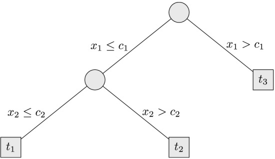
Example of a probability estimation tree for a dichotomous outcome y given covariates x ₁ and x ₂. Split points are c ₁ and c ₂, and the terminal nodes are labeled t ₁, t ₂, and t ₃.

For each terminal node, the probability estimate of the tree is the relative frequencies of subjects having the event in that terminal node. For example, for terminal node t ₁, the conditional probability to be estimated is

$$P(y=1|x_1\le c_1,x_2\le c_2),$$

where c ₁ and c ₂ are the split points in the tree.

The conditional probabilities can be estimated using a logistic regression model. To this end, a dummy variable is generated for each terminal node to indicate whether a subject resides in this terminal node or not. Specifically, a dummy variable d ₁ is created for the terminal node t ₁, and this dummy variable takes values

$$d_1=\left\{\begin{array}{cc}1& \text{if}{x}_1\le c_1,x_2\le c_2\\ 0& \text{else}.\end{array}\right.$$

Dummy variables d ₂ and d ₃ are defined for terminal nodes t ₂ and t ₃ accordingly:

$$d_2=\left\{\begin{array}{cc}1& \text{if}{x}_1\le c_1,x_2>c_2\\ 0& \text{else}\end{array}\right.\text{and}{d}_3=\left\{\begin{array}{cc}1& \text{if}{x}_1>c_1\\ 0& \text{else}\end{array}\right..$$

One of the three dummy variables d ₁, d ₂, d ₃ is taken as reference category, and we recommend choosing the one with the largest terminal node size. For each former tree, a logistic regression model is fitted, and the logistic regression model to be fitted for this tree is logit P(y = 1|d ₁,d ₂) = α + β ₁ d ₁+β ₂ d ₂ if d ₃ is used as reference category. The logistic regression model can be fitted either using the bootstrap sample drawn for this tree or using the entire training data. However, the results can be expected to be similar because the diversity of the models is already obtained from the bootstrap samples used for creating the random forest. We therefore decided to fit the logistic regression model on the entire training data for sake of simplicity. The conditional probabilities can be obtained for each terminal node from this logistic regression model.

All trees of the random forest are translated to a logistic regression model in the same way. The random forest can then be updated to a calibration data set by updating each of the logistic regression models using re‐calibration. For re‐calibration, the intercept of the logistic regression model is re‐estimated, while the other coefficients are kept unchanged 2. One assumption underlying this re‐calibration procedure is that the relative strength of the predictor variables is approximately similar in the two data sets. This means that the relative strength of combinations of variables represented by the dummy variables is approximately similar in both data sets. The procedure is summarized in Figure 2.

Figure 2.

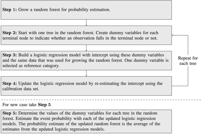
Steps in logistic regression‐based updating approach for random forests.

3.3. On the theoretical foundation of the two updating approaches

The mathematical basis for the validity of the two approaches differ: Elkan's approach relies on a formal argument using the Bayes formula. In contrast, the logistic regression‐based updating approach makes use of the fact that each terminal node represents a conditional probability, which can be estimated using logistic regression by providing the appropriate covariate. The idea of translating trees into a different form to obtain further improvements has been used before. For example, Seyedhosseini et al., 20 proposed to write the single trees as disjunctive normal forms. These can be optimized and result in disjunctive normal random forests with an improved performance compared with conventional random forests.

4. Simulation study

4.1. Data generation

To compare the two calibration methods in a simulation study, data were generated from two populations with different disease prevalences. Data from the first population were used for model building, and they are termed model‐building data. Data from the second population were split into training data and test data. These are named cal‐training data and cal‐test data, respectively.

Data sets were generated by means of logistic regression models. Covariates x ₁,…,x _p were generated according to predefined probability distributions. Regression coefficients β ₁,…,β _p and the intercept α were set to specific values. With these values, the probability for a positive event was estimated using the logistic regression model

$$\text{logit}P\left(y=1|x_1,\dots ,x_p\right)=\alpha +{\beta }_1{x}_1+\dots +{\beta }_p{x}_p.$$

The class of the outcome variable y was then assigned using a Bernoulli distribution with the previously calculated probability for a positive event.

In this simulation study, nine different scenarios were considered. In all simulation scenarios, the intercept was set to 0 for the model‐building data, and the intercept was set to 1 for the calibration data sets. The settings are summarized in Table 1. Continuous variables were generated according to a standard normal distribution, except for simulation scenarios 6 an 7. In these scenarios, the distribution of the continuous variable differed between the model‐building data and the calibration data. The five categorical variables in simulation scenarios 3 and 4 had k = 2,2,3,4,5 equally probable categories. The regression coefficients were identical in the model‐building data and the calibration data sets for all covariates in simulation scenarios 1–7. In simulation scenarios 8 and 9, the regression coefficient was 1 in the model‐building data. In the calibration data sets, the regression coefficients were 2 and 3, respectively. Noise variables without influence on the outcome were only simulated in simulation scenarios 2 and 4. They were continuous and generated from a standard normal distribution. In all simulation scenarios except simulation scenario 5, the number of observations in the model‐building data, the cal‐training data, and the cal‐test data was 1000 each. In scenario 5, the cal‐training data set was smaller and comprised only 100 observations. One hundred replications were generated for each simulation scenario.

Table 1.

Main settings in the simulation scenarios.

Scenario	Cont	Cat	Noise	Distinctive feature
1	2	0	0	–
2∗	2	0	8	–
3∗	5	5	0	–
4	5	5	90	–
5	2	0	0	Smaller calibration data set for training
6	1	0	0	Unequal covariate distribution: MB $\mathcal{N}(0,1)$, Cal $\mathcal{N}(-0.75,0.5)$
7	1	0	0	Unequal covariate distribution: MB $\mathcal{N}(1,1)$, Cal $\mathcal{N}(-1,1)$
8	1	0	0	Unequal coefficients: MB β = 1, Cal β = 2
9	1	0	0	Unequal coefficients: MB β = 1, Cal β = 3

Cont, number of continuous covariates; Cat, number of categorical covariates; Noise, number of noise variables; MB, model‐building data; Cal, calibration data; Distinctive feature, additional distinctive feature, if applicable.

^∗Results shown in Supporting Information.

For all random forests, 200 trees were grown with a terminal node size of 10% of the total sample size. Default settings were used for all other parameters. First, a random forest for probability estimation was grown using the model‐building data (RF). Second, the RF was translated to logistic regression models, which were fitted using the model‐building data (RF + LogReg). These were then updated by re‐estimating the intercept 2 using the cal‐training data (RF + LogReg + Cal). Fourth, the probability estimates of RF were updated using Elkan's method with base rates calculated from the model‐building data and the cal‐training data (RF + CalElkan). Fifth, a random forest for probability estimation was grown using the cal‐training data (RF onCalData). Sixth, a logistic regression model was fitted using the model‐building data and re‐calibrated using the cal‐training data (LogReg + Cal). All models were compared on the cal‐test data. We used the statistical software R for analysis 21 and the R package ranger for building the random forests 22.

4.2. Results

Figure 3 displays true versus predicted probabilities for simulation scenario 1. First of all, we note that both random forest‐based calibration approaches work. As expected, random forests did not perform as good as logistic regression because data were generated according to a logistic regression model with linear main effects only without interactions. However, for other simulated data sets, random forests outperformed logistic regression 9. One such example is data generated according to the Mease 23 model (Figure S1).

Figure 3.

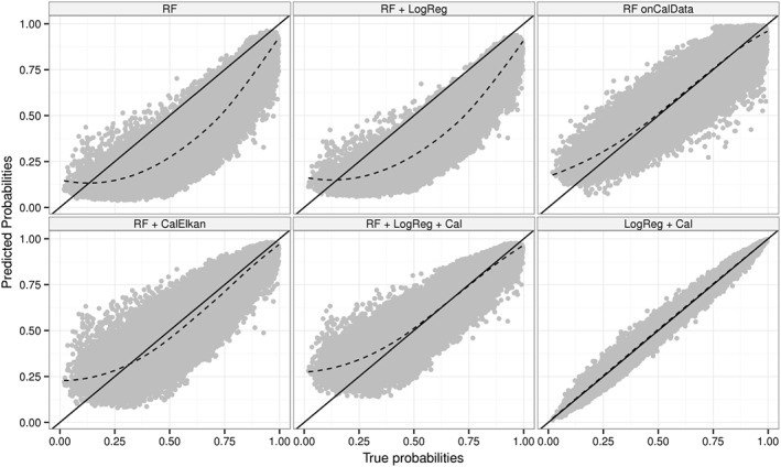
True versus predicted probabilities for simulation scenario 1. RF: random forest built on model‐building data; RF + LogReg: RF translated to logistic regression models; RF + LogReg + Cal: RF + LogReg updated using re‐calibration; RF + CalElkan: probabilities from RF updated using Elkan's method; RF onCalData: random forest built on cal‐training data; LogReg + Cal: logistic regression fitted using model‐building data and updated using re‐calibration.

Elkan's method and the logistic regression‐based approach decreased the MSE in simulation scenario 1 compared with the initial random forest (Figure 4). The MSEs were comparable. Results were similar for simulation scenarios 2 and 3 (Figure S9) and for the random forest‐based approaches in simulation scenario 4. The re‐calibrated logistic regression performed worse in simulation scenario 4, in which many noise variables were present. In scenarios 1–4, the covariate distributions and coefficients were identical in the model‐building data and the calibration data. In simulation scenarios 1–4, the MSEs of both updating approaches were similar to the MSE of the random forest built on the cal‐training data. However, in simulation scenario 5, both updating approaches performed better than the random forest built on the cal‐training data (Figure 5) because the cal‐training data were substantially smaller than in the other simulation scenarios.

Figure 4.

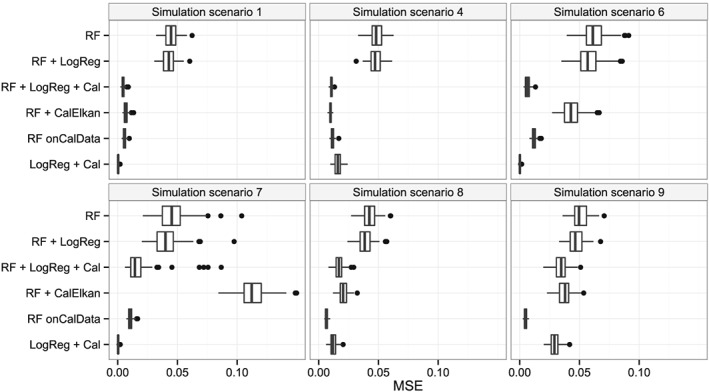
Mean‐squared errors between true and predicted probabilities in the simulation study. RF: random forest built on model‐building data; RF + LogReg: RF translated to logistic regression models; RF + LogReg + Cal: RF + LogReg updated using re‐calibration; RF + CalElkan: probabilities from RF updated using Elkan's method; RF onCalData: random forest built on cal‐training data; LogReg + Cal: logistic regression fitted using model‐building data and updated using re‐calibration.

Figure 5.

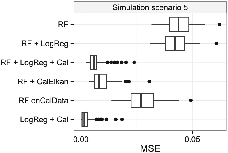
Mean‐squared errors between true and predicted probabilities in simulation scenario 5, where the calibration data for training were substantially smaller than in the other simulation scenarios. RF: random forest built on model‐building data; RF + LogReg: RF translated to logistic regression models; RF + LogReg + Cal: RF + LogReg updated using re‐calibration; RF + CalElkan: probabilities from RF updated using Elkan's method; RF onCalData: random forest built on cal‐training data; LogReg + Cal: logistic regression fitted using model‐building data and updated using re‐calibration.

Figure 6 displays true versus predicted probability estimates and shows that Elkan's method did not adequately update probabilities in simulation scenario 6. Figure 4 depicts the corresponding MSEs, which are substantially larger for Elkan's method than the MSE for the logistic regression‐based re‐calibration approach. In fact, the covariate distribution was unequal for the model‐building data and calibration data in simulation scenario 6. The assumptions underlying Elkan's method were thus not met. Unequal covariate distributions were also generated in simulation scenario 7. However, the ranges of the covariate differed substantially between both data sets in this extreme scenario. As a result, Elkan's method failed in this simulation scenario 7. The probability estimates updated using Elkan's method were even further away from the ideal line than the probability estimates of the initial random forest (Figure S6). The logistic regression‐based updating approach seemed to perform well. However, for some trees, the corresponding logistic regressions did not converge in this extreme scenario. The MSEs for the logistic regression‐based updating approach and the random forest built on the cal‐training data were similar for simulation scenarios 6 and 7.

Figure 6.

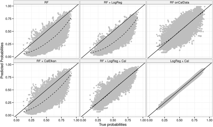
True versus predicted probabilities for simulation scenario 6. RF: random forest built on model‐building data; RF + LogReg: RF translated to logistic regression models; RF + LogReg + Cal: RF + LogReg updated using re‐calibration; RF + CalElkan: probabilities from RF updated using Elkan's method; RF onCalData: random forest built on cal‐training data; LogReg + Cal: logistic regression fitted using model‐building data and updated using re‐calibration.

Finally, the effect sizes of the covariate differed between the model‐building data and the calibration data in simulation scenarios 8 and 9. Both updating approaches for random forest and the re‐calibrated logistic regression did not perform as good as the random forest built on the cal‐training data. However, the difference was moderate in simulation scenario 8, and it was substantially larger in simulation scenario 9. Here, the effect size varied considerably between the model‐building and the calibration data sets.

For sensitivity analysis, we performed the same analyses with random forests grown with a terminal node size of 5% and 15% of the total sample size. Results were comparable (Figures S10 and S11).

5. Real data analysis: predicting functional outcome after stroke

The two updating approaches were also applied to real data for prognosis 90 days after stroke. The study has been described in detail elsewhere 24, 25, 26. In brief, the training data comprising 1754 subjects with ischemic stroke was prospectively collected from 23 neurology departments in 1998 and 1999. All participating hospitals had an acute stroke unit. Patients for validation were enrolled during 2001 and 2002. Nine hospitals participated in the validation study only, allowing for a combined temporal and external validation in a sample of 874 patients. Four additional hospitals also participated in the initial study, and these provided data for temporal validation from 596 patients. Patients were informed about study participation, and all patients gave informed consent if their personal data were to be transferred to the data management center. The study was approved by the Ethics Committee of the University of Essen, Germany. Prior to analysis, missing values were imputed using mean or mode imputation.

The aim was to construct a model for complete restitution versus incomplete restitution or mortality. The Barthel index (BI) 27 assesses functional independence. It measures individual abilities related to feeding, dressing, mobility, and personal hygiene. Complete restitution was assumed for individuals with BI $\ge 95$ and incomplete restitution for individuals with BI <95. As before 24, we used all 34 variables for prediction that were available for the training data and the validation data. Descriptive statistics of the variables that were previously identified by logistic regression models using the same data 25 are summarized in Table 2. This table indicates that the distribution differs between the training data and the temporal and external validation data for some covariates, such as fever.

Table 2.

Patient characteristics in the stroke data. n (%) are displayed for dichotomous variables, mean and standard deviation (SD) for continuous variables.

Variable	Training data	Temporal validation	External validation
Barthel index after 90 days: $\ge 95$	1025(58.4%)	337(56.5%)	494(56.5%)
Survival after 90 days: Yes	1588(90.5%)	546(91.6%)	811(92.8%)
Prior stroke: Yes	353(20.1%)	137(23.0%)	172(19.7%)
Diabetes mellitus: Yes	436(24.9%)	165(27.7%)	229(26.2%)
Lenticulostriate arteries infarction: Yes	188(10.7%)	31(5.2%)	64(7.3%)
Fever: Yes	220(12.5%)	51(8.6%)	54(6.2%)
Neurological complications: Yes	73(4.2%)	26(4.4%)	37(4.2%)
Gender: Female	716(40.8%)	270(45.3%)	357(40.8%)
Age at event (in years)	68.1(12.7)	68.0(12.4)	67.8(12.4)
NIHSS left arm	0.6(1.2)	0.6(1.1)	0.6(1.2)
NIHSS right arm	0.7(1.2)	0.5(1.1)	0.6(1.1)
NIHSS total score	6.9(6.2)	6.1(5.7)	6.6(6.1)
Rankin Scalea	3.1(1.4)	2.4(1.6)	2.5(1.6)

NIHSS: National Institutes of Health Stroke Scale.

^aOverall functional impairments as rated on the Modified Rankin Scale 48–72 h after admission.

A random forest for probability estimation was built using the stroke training data. The number of trees ntree was set to 200, the terminal node size nodesize was set to 10%, and the number of variables available for splitting at a node was set to mtry=9. Default settings were used for all other parameters. We used 10‐fold cross‐validation when we updated the random forest to the validation data for both random forest‐based re‐calibration methods. Specifically, we compared the probability predictions for the validation data of the initial random forest (RF), the random forest updated using Elkan's method (RF + CalElkan), and the random forest updated using the logistic regression‐based approach (RF + LogReg + Cal). Calibration curves were used for evaluation. To this end, the average number of observations per group was set to 50 for grouped proportions. The analyses were carried out using R 21, the R package ranger for building the random forests 22 and the R package rms for plotting the calibration curves 28.

The probability estimates of the random forest updated using the logistic regression‐based updating approach were closer to the ideal line than the probability estimates from the initial random forest and the probability estimates updated by Elkan's method for the external validation data (Figure 7). The Brier score with 95% bootstrap confidence intervals (in brackets) after 2000 bootstrap draws was 0.169 [0.154;0.183] for the probability estimates of the initial random forest. It was slightly decreased to 0.167 [0.153;0.181] by updating using Elkan's method, and it was lowered to 0.163 [0.151;0.176] for the probability estimates updated using the logistic regression‐based approach.

Figure 7.

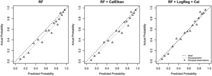
Calibration curves for external stroke validation data. RF: random forest built on training data; RF + CalElkan: probabilities from RF updated using Elkan's method; RF + LogReg + Cal: RF translated to logistic regression models and updated using re‐calibration.

These findings were confirmed by the temporal validation data (Figure S12). The Brier scores were 0.157 [0.140;0.174] for the initial random forest, 0.156 [0.138;0.172] for Elkan's method, and 0.150 [0.135;0.164] for the logistic regression‐based updating approach. The calibration curves for a logistic regression and a re‐calibrated logistic regression model (Figures S13 and S14) look similar to the calibration curves for the initial random forest and the random forest updated using the logistic regression‐based approach.

6. Discussion

Elkan's method for updating random forests and the logistic regression‐based updating approach for random forests are both valid for re‐calibration. The latter method is preferable to Elkan's method when the covariate distribution is unequal in the two data sets. This became apparent in simulation scenario 6 as well as in the real data analysis. In the real data example, some covariates differed in their distribution between the training and the validation data, and the calibration curves and Brier scores indicated a better performance of the logistic regression‐based approach than of Elkan's method. In simulation scenario 6, the probability estimates updated using Elkan's method were worse compared with the probability estimates updated using the logistic regression‐based updating approach. In this simulation scenario, the covariate distribution differed between the model‐building data and the calibration data. Elkan's method only takes the base rates into account, and this may explain the differences. For equally distributed covariates, the base rate in the calibration data would have been larger than in the model‐building data. However, in simulation scenario 6, the model‐building data had a higher frequency of covariate values with higher event probabilities than the calibration data. As a result, the difference in base rates was smaller, and the probability estimates were not adequately calibrated using Elkan's approach.

Updating an existing predictive model is advantageous compared with completely new estimation if only a small data set is available for calibration. Both approaches performed similarly in this case, and both re‐calibration methods performed well (Figure 5). One reason for this is that information from the model‐building data is still used in addition to the calibration data set. This is especially meaningful if only a small calibration data set is available 2, 29. However, updating a previously developed model is not always possible. Especially if a large calibration data set is available, it might be better to discard a poorly performing model 2, 30. Compared with the use of both updating approaches, it might also be preferable to completely re‐estimate a model if the relative strength of the predictor variables varies considerably between the training and the calibration data sets (simulation scenario 9).

Once the logistic regressions have been fitted, the set of logistic regressions can be converted back to a random forest. Each logistic regression was estimated on the basis of a single tree in the random forest. The class probability of each terminal node obtained from the logistic regression is used as new class probability for that terminal node in the tree. This conversion of the logistic regression back to a random forest might save computation time for probability estimation because subjects just need to be dropped down a tree to obtain the final estimate in a tree.

Our simulation studies have several limitations. Specifically, we neither investigated the effect of the terminal node size on the performance of the two re‐calibration methods comprehensively, nor the effect of the number of trees nor the number of variables available for splitting at a parent node in the random forest. In fact, the terminal node size could be tuned as described elsewhere 12. Similarly, the optimal number of covariates available for splitting could be tuned 31. Finally, the optimal number of trees could be determined in a two‐step procedure 32. However, all these approaches are computer processor time‐intensive. For sensitivity analysis, we repeated the analysis with two different terminal node sizes yielding similar results. Furthermore, the simulation studies have demonstrated that both approaches for re‐calibrating random forests are valid if the underlying assumptions are met.

For both the simulated data and the stroke data, it was reasonable to use re‐calibration for updating the logistic regression models of the translated random forests. This approach relies on the assumption that the effect of predictors is approximately similar in the model‐building and calibration data. More extensive updating strategies, allowing for adjustments of relative effects, relax this assumption 2. However, for the simulated data and the stroke data, it was plausible to assume similar effects of the predictors in the two data sets. We stress that re‐calibration is especially useful if only a small data set is available for calibration. In this case, more extensive updating approaches may even harm predictive performance 2.

In summary, we have proposed a new logistic regression‐based updating approach for random forests for probability estimation that has weaker assumptions than Elkan's method. Elkan's approach has the advantage that it can be applied to any probability machine. In contrast, the logistic regression‐based approach is especially designed for updating random forests for probability estimation. Both approaches are simple to implement in standard software packages. R code is available in the Supporting Information so that both methods can be used in applications.

Conflicts of interest

AZ serves as associate editor for Statistics in Medicine.

Supporting information

Supporting info item

Dankowski, T. , and Ziegler, A. (2016) Calibrating random forests for probability estimation. Statist. Med., 35: 3949–3960. doi: 10.1002/sim.6959.

References

- 1. Justice AC, Covinsky KE, Berlin JA. Assessing the generalizability of prognostic information. Annals of Internal Medicine. 1999; 130(6):515–524. [DOI] [PubMed] [Google Scholar]
- 2. Steyerberg EW, Borsboom GJJM, van Houwelingen HC, Eijkemans MJC, Habbema JDF. Validation and updating of predictive logistic regression models: a study on sample size and shrinkage. Statistics in Medicine. 2004; 23(16):2567–2586. [DOI] [PubMed] [Google Scholar]
- 3. Boström H. Calibrating random forests. In Proceedings of the Seventh International Conference on Machine Learning and Applications: Piscataway, NJ, 2008; 121–126. [Google Scholar]
- 4. Breiman L. Random forests. Machine Learning. 2001; 45(1):5–32. [Google Scholar]
- 5. Breiman L, Friedman J, Olshen RA, Stone CJ. Classification and Regression Trees. Chapman & Hall/CRC: Boca Raton, FL, 1984. [Google Scholar]
- 6. Arlot S, Genuer R. Analysis of purely random forests bias, 2014. arXiv preprint arXiv:1407.3939.
- 7. Biau G. Analysis of a random forests model. The Journal of Machine Learning Research. 2012; 13: 1063–1095. [Google Scholar]
- 8. Malley JD, Kruppa J, Dasgupta A, Malley KG, Ziegler A. Probability machines: consistent probability estimation using nonparametric learning machines. Methods of Information in Medicine. 2012; 51(1):74–81. [DOI] [PMC free article] [PubMed] [Google Scholar]
- 9. Kruppa J, Liu Y, Biau G, Kohler M, König IR, Malley JD, Ziegler A. Probability estimation with machine learning methods for dichotomous and multicategory outcome: theory. Biometrical Journal. 2014; 56(4):534–563. [DOI] [PubMed] [Google Scholar]
- 10. Steinberg D. 2009. CART: Classification and regression trees In The top Ten Algorithms in Data Mining, Wu X, Kumar V. (eds). Chapman & Hall/CRC: Boca Raton, FL; 179–201. [Google Scholar]
- 11. Elkan C. The foundations of cost‐sensitive learning. In Proceedings of the Seventeenth International Joint Conference on Artifical Intelligence: San Francisco, CA, 2001; 973–978. [Google Scholar]
- 12. Kruppa J, Schwarz A, Arminger G, Ziegler A. Consumer credit risk: individual probability estimates using machine learning. Expert Systems With Applications. 2013; 40(13):5125–5131. [Google Scholar]
- 13. Biau G, Devroye L, Lugosi G. Consistency of random forests and other averaging classifiers. The Journal of Machine Learning Research. 2008; 9: 2015–2033. [Google Scholar]
- 14. Genuer R. Variance reduction in purely random forests. Journal of Nonparametric Statistics. 2012; 24(3):543–562. [Google Scholar]
- 15. Lin Y, Jeon Y. Random forests and adaptive nearest neighbors. Journal of the American Statistical Association. 2006; 101(474):578–590. [Google Scholar]
- 16. Kruppa J, Ziegler A, König IR. Risk estimation and risk prediction using machine‐learning methods. Human Genetics. 2012; 131(10):1639–1654. [DOI] [PMC free article] [PubMed] [Google Scholar]
- 17. Stanski HR, Wilson LJ, Burrows WR. Survey of common verification methods in meteorology, WMO world weather watch technical report 8, wmo/td no. 358, Melbourne, 1989. Available from: http://www.cawcr.gov.au/ projects/verification/Stanski_et_al/Stanski_et_al.html [accessed February 18, 2016]. [Google Scholar]
- 18. Gneiting T, Raftery AE. Strictly proper scoring rules, prediction, and estimation. Journal of the American Statistical Association. 2007; 102(477):359–378. [Google Scholar]
- 19. Bradley AA, Schwartz SS, Hashino T. Sampling uncertainty and confidence intervals for the Brier score and Brier skill score. Weather and Forecasting. 2008; 23(5):992–1006. [Google Scholar]
- 20. Seyedhosseini M, Tasdizen T. Disjunctive normal random forests. Pattern Recognition. 2015; 48(3):976–983. [Google Scholar]
- 21. R Core Team. R: a language and environment for statistical computing. R Foundation for Statistical Computing: Vienna, Austria, 2014. Available from: http://www.R-project.org/ [accessed: 28 March 2016]. [Google Scholar]
- 22. Wright MN. ranger: a fast implementation of random forests, 2016. Available from: http://CRAN.R-project.org/ package=ranger R package version 0.3.0 [accessed: 28 March 2016].
- 23. Mease D, Wyner AJ, Buja A. Boosted classification trees and class probability/quantile estimation. The Journal of Machine Learning Research. 2007; 8: 409–439. [Google Scholar]
- 24. König IR, Malley JD, Weimar C, Diener HC, Ziegler A. on behalf of the German Stroke Study Collaboration. Practical experiences on the necessity of external validation. Statistics in Medicine. 2007; 26(30):5499–5511. [DOI] [PubMed] [Google Scholar]
- 25. Weimar C, Ziegler A, König IR, Diener HC. on behalf of the German Stroke Study Collaborators. Predicting functional outcome and survival after acute ischemic stroke. Journal of Neurology. 2002; 249(7):888–895. [DOI] [PubMed] [Google Scholar]
- 26. Weimar C, König IR, Kraywinkel K, Ziegler A, Diener HC. on behalf of the German Stroke Study Collaboration. Age and National Institutes of Health Stroke Scale Score within 6 hours after onset are accurate predictors of outcome after cerebral ischemia: development and external validation of prognostic models. Stroke. 2004; 35: 158–162. [DOI] [PubMed] [Google Scholar]
- 27. Mahoney FI, Barthel DW. Functional evaluation: the Barthel index. Maryland State Medical Journal. 1965; 14: 56–61. [PubMed] [Google Scholar]
- 28. Harrell Jr FE. rms: regression modeling strategies, 2016. Available from: http://CRAN.R-project.org/package=rms R package version 4.4‐2 [accessed: 26 March 2016].
- 29. Janssen KJM, Moons KGM, Kalkman CJ, Grobbee DE, Vergouwe Y. Updating methods improved the performance of a clinical prediction model in new patients. Journal of Clinical Epidemiology. 2008; 61(1):76–86. [DOI] [PubMed] [Google Scholar]
- 30. Altman DG, Royston P. What do we mean by validating a prognostic model? Statistics in Medicine. 2000; 19(4):453–473. [DOI] [PubMed] [Google Scholar]
- 31. Schwarz DF, König IR, Ziegler A. On safari to random jungle: a fast implementation of random forests for high dimensional data. Bioinformatics. 2010; 26(14):1752–1758. [DOI] [PMC free article] [PubMed] [Google Scholar]
- 32. Lopes M. Measuring the convergence rate of random forests via the bootstrap. In Joint Statistical Meeting: Seattle, United States of America, 2015. Available from: https://www.amstat.org/meetings/jsm/2015/onlineprogram/ AbstractDetails.cfm?abstractid=317640 [accessed: 26 March 2016]. [Google Scholar]
Associated Data
This section collects any data citations, data availability statements, or supplementary materials included in this article.
Supplementary Materials