Abstract.
Quantitative histomorphometry (QH) is the process of computerized feature extraction from digitized tissue slide images to predict disease presence, behavior, and outcome. Feature stability between sites may be compromised by laboratory-specific variables including dye batch, slice thickness, and the whole slide scanner used. We present two new measures, preparation-induced instability score and latent instability score, to quantify feature instability across and within datasets. In a use case involving prostate cancer, we examined QH features which may detect cancer on whole slide images. Using our method, we found that five feature families (graph, shape, co-occurring gland tensor, sub-graph, and texture) were different between datasets in 19.7% to 48.6% of comparisons while the values expected without site variation were 4.2% to 4.6%. Color normalizing all images to a template did not reduce instability. Scanning the same 34 slides on three scanners demonstrated that Haralick features were most substantively affected by scanner variation, being unstable in 62% of comparisons. We found that unstable feature families performed significantly worse in inter- than intrasite classification. Our results appear to suggest QH features should be evaluated across sites to assess robustness, and class discriminability alone should not represent the benchmark for digital pathology feature selection.
Keywords: quantitative histomorphometry, prostate cancer, feature stability, site variation, digital pathology, stain variability, prognosis, machine learning
1. Introduction
Quantitative histomorphometry (QH) is the process of computerized extraction of features from digitized slide images.1–12 These features are typically then used with automated classification methods to predict disease presence, behavior, and outcome. A major challenge for QH is the variation among pathology images across multiple sites. This variation is induced in the preparation phase prior to computational image analysis when tissue samples are stained, mounted onto a glass slide, and subsequently digitized via a whole slide scanner. Stain concentration, manufacturer, and batch effects affect the final appearance of a slide.13 In addition, the specific whole slide scanner used to digitize a slide can affect the appearance of the final digital image. All these preparation-induced image variations can affect the automated analysis of the image and thus the calculated feature values.
Image variation affects the features computed from an image and thus poses a problem for diagnostic and predictive algorithms based on these features. A key step in using these algorithms is choosing which features to use for classification. Traditional classification-based performance measures such as accuracy and area under the receiver operating characteristic curve are typically employed in feature selection methods that aim to identify features that maximize class discriminability. But to create a robust classifier, the feature selection algorithm must consider both discrimination and stability. A feature is stable if the mean and shape of its distribution is consistent among cohorts of patients who share disease or clinical profiles or outcomes. While feature stability has been examined in the radiology space,14–17 relatively little work has been done in the context of QH or in digital pathology.
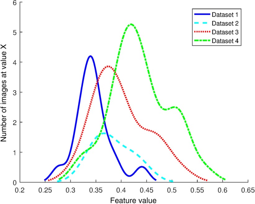
Cross institutional color variation is a well-known problem in digital pathology as evidenced by the large number of methods developed to quantify image color and standardize images to a template.18–21 While standardization of stains and procedures as suggested in Lyon et al.13 could help reduce variation, logistical and physical limitations mean that digital color correction will always be needed to ensure uniform color. Color normalization (CN) is broadly the process of altering the color channel values of pixels in a source image so that its color distribution matches that of a template image. Since image color is affected by preparation procedure and thus is a possible contributor to feature instability, one needs to evaluate the effect of CN on the resulting feature expression values. Some work has been done to evaluate the effect of CN on classifier performance in applications such as mitosis detection,18 but to our knowledge no study has been performed which examines the link between CN and feature values or feature stability. Staining and scanning procedures should not, in an ideal setting, dramatically affect the value of a stable feature. An example of an unstable feature is shown in Fig. 1. The feature value distributions from four datasets are shown to be of similar shape but with different means and modes.
Fig. 1.
Smoothed distribution of graph feature “disorder of nearest neighbor in 20 pixel radius” from the nonrecurrence Gleason 7 patients of four datasets.
In this paper, we investigate the effect of feature instability on classification, introduce a method for quantifying feature stability across many digital pathology datasets, and determine instability specifically resulting from use of different whole-slide scanners. To examine the degree to which site variability affects feature accuracy, we investigated the degradation of classifier performance in the context of intra- and intersite classification of tumor and nontumor regions of prostate tissue for 81 patients. Stability is evaluated using two feature-based evaluation measures. The first stability evaluation measure, latent instability (LI) score, aims to evaluate the inherent randomness of a feature’s distribution within a single-preparation procedure from factors such as interpatient feature variation. A low LI would indicate that intradataset variation is very low and that there is a low probability of features being different between two datasets with similar disease or clinical profiles or outcome due to random chance. We also introduce a method involving cross-dataset comparisons for quantifying the frequency at which a feature is different between datasets via a preparation-induced instability (PI) score. A high PI would indicate that a feature is affected by preparation procedures. Lastly, we apply these methods to a use case involving detecting tumor and nontumor regions on radical prostatectomy (RP) samples taken from prostate cancer patients based off QH analysis of digitized images. Our group has previously investigated the role of a number of different histomorphometric features including gland and nuclear shape, morphology, orientation, and disorder with prostate cancer presence, grade, aggressiveness, and outcome.22–29 The goal of this study is to identify which of these classes of features, which are predictive of presence of prostate cancer, are most stable across sites and scanners. Specifically, in this paper, we examine the stability of 216 gland lumen and 26 texture features extracted from 80 whole mount prostate adenocarcinoma (CaP). Our goal was to compare the intra- and interdataset variations of the prostate histology QH features to determine if the QH variance across sites is significantly larger than might be expected due to random chance.
We applied CN to the four datasets and measure feature instability among datasets before and after normalization. The goal of the experiment was to gain some insight into the potential of CN as a technique for reducing feature instability among datasets. We scanned the 34 slides of a single dataset on three different scanners to examine the specific contribution of scanner variation to feature instability. While clearly there are multiple sources of variance affecting the stability of image features, in this paper, we focus on two critical aspects in digital pathology, color variance due to differences in site and slide digitization and the induced color variation on account of different scanners.
Thus our contributions in this paper are
-
•
A method for evaluating precisely how histomorphometric features tend to vary across sites with varying preparation procedures.
-
•
New quantitative measures to evaluate feature stability across and within datasets, as well as quantitatively assessing the effect of CN on the resulting feature expression.
-
•
An evaluation of the stability of 242 QH features from five feature families in prostate histology across sites before and after CN and across whole-slide scanners.
The rest of this paper is organized as follows. Section 2 introduces the new metrics used to evaluate feature stability. Section 3 describes how feature instability affects classification and the CN, segmentation, and feature extraction techniques employed. Section 4 lays out the experimental design and quantitative results. Section 5 concludes the paper with a summary of the study and closing remarks.
2. Feature Robustness Indices
2.1. Latent Instability Score
To create a baseline for the expected feature value variation between images we compared feature distributions within random splits of a dataset , , , . Random halves of were compared against each other to check for significant differences in feature distribution between the halves. The end result of this process is a calculation of a feature’s LI score which represents the probability that a feature will be different among datasets due to effects not linked to the specific laboratory. Random dataset splits used to calculate LI produce subsets that contain different patients with different image content. LI is a measure of a feature’s inherent variability and the degree to which interpatient variance may contribute to feature instability when measured across datasets.
We split images , , where is the number of images in dataset into two equal parts , , for , where refers to the number of splitting iterations. and are sets of images such that the subsets are unique, all .
From the set of all features , we examined one feature at a time, , , is the total number of features. We computed the LI of in by taking the percentage of splits where the vector of feature values and were statistically significantly different under the Wilcoxon rank sum test (U), such that
| (1) |
where , and is the feature representation of the ’th feature of all the images in and , and is the -value of U in iteration . U was chosen due to its resilience to the effect of outliers and its ability to handle unknown distributions. Feature distributions were considered to be significantly different if they were different at the confidence level. is equal to the percentage of splits in which feature was significantly different between halves of . Therefore .
2.2. Preparation-Induced Instability Score
The feature values of two cohorts were compared using U. A pairwise comparison of each combination of datasets , was performed over trials using a random three-quarters of each dataset, creating and for every iteration for a total of comparisons per feature. From these comparisons, PI was calculated as a quantitative measure of the sensitivity of a feature to staining and scanning procedures. While LI measures how often a feature would be expected to be different among datasets without any differences among laboratories, PI represents how often that feature was actually found to be different among datasets. The difference between a feature’s LI and PI thus reveals the effect of laboratory preparation procedure on that feature.
| (2) |
is equal to the percentage of pairwise comparisons in which was significantly different among datasets. A high PI paired with a low average LI suggests that the feature is different among datasets due to fundamental differences among the datasets rather than noise inherent in the feature or interpatient variability.
3. Methods and Materials
3.1. Significance of Feature Instability
To determine the effect of feature instability and link the image extracted features to a specific task, we performed an experiment to test classification of tumor and benign regions in RP specimens. As all the RP patients had prostate cancer, the benign regions were selected from the noncancerous zones of those specimens. A total of 81 patients from two sites were used for this classification experiment. Dataset information is provided in Table 1. To determine the effect of using feature families of varying stability, classification experiments were performed using each feature family separately and with all 242 features. The results of cross-validation within a single site and independent validation across sites were compared with the hypothesis that unstable features would perform better in intrasite classification than in intersite tasks where feature instability would adversely affect model generalizability. Features were selected using the Wilcoxon rank-sum significance test between the tumor and benign regions of the training set at the significance level. For patients with multiple tumor or benign regions, only the largest region of each class was used. Classification was performed using a random forest classifier30 with 50 trees over 100 iterations. In each fold of cross validation, a random two-thirds of a site’s patients were used for training with the remaining third used for validation, with all regions of every patient kept in the same set. Significant features were selected on the training data independently in each fold.
Table 1.
Patients used for cancerous and noncancerous region classification.
| Total patients | 40 | 41 |
| With tumor regions only | 5 | 3 |
| With tumor and benign regions | 35 | 38 |
3.2. Statistical Analysis of Feature Robustness Indices
The purpose of the LI experiment was twofold. First, a low provides confirmation that is relatively consistent within . By looking only within a single dataset, we were able to partially control for the staining and scanning procedures and hence potentially identify if there were features that were inherently noisy even without additional confounding sources of variation. Second, the frequency of feature difference between the halves of the datasets allowed for establishment of a baseline for how often a feature would appear different between two sets due to random chance. This baseline is the measure by which we may judge interdataset feature instability. If a distribution was rarely different between the two halves of , it would appear unlikely that the feature distribution would be different across two different datasets.
A number of confounders affect the interpretation of the PI results, among them the difference in image content among the four patient cohorts. We have controlled for some clinical factors which may affect the resulting features (Gleason sum and patient outcome). The evidence of site-variation affecting stability may be assessed by comparing LI and PI results. Both LI and PI are arrived at by comparing unique sets of patients. However, while LI involves comparing patients from the same site, PI involves comparing images across sites. LI reflects the contribution of interpatient variation to feature instability while PI includes both patient variation and site-specific variation. Hence the ratio of PI to LI reflects the contribution of site variation to increased feature instability, a ratio that allows for the isolation of the site-induced variability from the image-specific variations. Further there are a number of factors that are not controlled for in the PI experiment, including image compression and original image magnification. However, in not controlling for these factors, we are following data acquisition protocols typical in digital pathology and which may be encountered in a typical clinical setting. Our findings suggest that greater attention to standardization of slide preparation, digitization, and analysis may be needed.
3.3. Color Normalization
We employed the nonlinear stain mapping CN method described by Khan et al.18 to normalize the color of the slide images. This method maps each stain in the source and template image to a channel, normalizes the channels, and then converts the image back to the RGB space. Other methods commonly used for hematoxylin and eosin (H&E) image normalization such as histogram color matching31 normalize the RGB channels themselves rather than using stain channels. However, this has the disadvantage of possibly inducing artifacts in the image.18 In our case, these artifacts severely degrade the performance of automated gland identification methods and thus necessitate the use of a stain channel approach. The images in dataset were color normalized to create dataset .
3.4. Segmentation
Gland lumen were automatically segmented from digital images of the cancerous regions of RP whole mount slide images using the approach described in Nguyen et al.32 To segment lumen, the algorithm first performed -means clustering of the colors of 10,000 randomly selected pixels in an image with . Pixels were given a label based on their cluster to define the prototypical color of nuclei, stroma, cytoplasm, and lumen in an image. These prototypes were then applied to the entire image to identify objects. Lumen objects surrounded by nuclei objects were deemed to be glands and the boundaries of the lumen were segmented.
3.5. Feature Extraction and Analysis
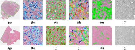
A total of 216 gland lumen features were extracted from segmented gland lumen after resizing segmentation results and images to magnification. Twenty-six Haralick features were extracted from the pixel intensity values of the entire image and involved excluding pixels corresponding to the gland segmentations. The extracted features belonged to five different families and are described in Table 2. A visualization of the five feature families is shown in Fig. 2. These features were chosen for analysis based on their relevance to CaP recurrence prediction as described in previous work from our group.6,33 Gland features are related to disease aggressiveness since more aggressive prostate cancer degrades the cohesiveness and regularity of the glands. These 216 features attempt to quantitatively capture gland morphology, shape, arrangement, and disorder of glands in the image. Since these features are intended to differentiate cancerous and noncancerous cases and images corresponding to different Gleason grades, there is a need to identify features that are stable and consistent.
Table 2.
Summary of features examined.
| Family | Description | Features |
|---|---|---|
| Graph | Descriptors of Delaunay, Voronoi, and minimum spanning tree diagrams | 51 |
| Shape | Lumen shape, smoothness, invariant moments, and Fourier descriptors | 100 |
| CGT6 | Entropy of gland orientation and neighborhood disorder | 39 |
| Subgraph | Local subgraph connectivity and distance between nodes | 26 |
| Texture | Relative pixel intensity, contrast, entropy, and energy | 26 |
Fig. 2.
Segmentation and feature visualization for (a–f) an image in and (g–l) an image in . (a, g) Cancerous regions annotated by expert pathologist. Automatically extracted features corresponding to (b, h) gland shape, (c, i) global gland graphs, (d, j) gland disorder, (e, k) local gland graphs, and (f, l) Haralick intensity texture.
The 51 graph-based features captured the spatial arrangement of the glands as calculated by using gland centroids as vertices. These include first- and second-order descriptors of Voronoi diagrams [see Figs. 2(c) and 2(i)], Delaunay triangulations, minimum spanning trees, and gland density.6
The 100 gland shape features measured the average shape of all the glands in an image as described by the lumen boundaries and the resulting area, perimeter, distance, smoothness, and Fourier descriptors.23
The 39 co-occurring gland tensor (CGT) features measured the disorder of neighborhoods of glands as measured by the entropy of orientation of the major axes of glands within a local neighborhood.6 Gland orientations can be visualized in Figs. 2(d) and 2(j), where the gland boundaries are color coded based on the angle of their orientation.
The 26 subgraph features described the connectivity and clustering of small gland neighborhoods using gland centroids [see Figs. 2(e) and 2(k)].5
The 26 Haralick texture features measured second-order intensity statistics.34 These features do not explicitly rely on gland segmentations.
3.6. Dataset Description
We collected 146 H&E-stained whole mount prostate tissue RGB images for the purpose of detecting cancerous regions on RP specimens. A series of QH features (as described in Sec. 3) previously shown to be predictive of biochemical recurrence of prostate cancer were extracted. Two separate cohorts from the University of Pennsylvania contained 41 and 40 patients, respectively ( and ). The Cancer Genome Atlas35 provided two datasets, 32 patients from the University of Pittsburgh () and 33 from Roswell Park (). All images were digitized using a whole slide scanner. The images within and were available in their digital form from the TCGA. and were originally digitized at magnification on an Aperio CS2 scanner. The precise make and model of the scanner used for the cases in and was not known; however, they were originally digitized at magnification. For each patient, a representative cancerous region of interest was identified and annotated by an expert pathologist. Features were calculated from within the annotated region. All images in all experiments were downsized to magnification ( per pixel) for gland segmentation and ( per pixel) for feature extraction.
3.6.1. Feature stability experiment
To investigate the stability of these features, we controlled the populations across the datasets and matched 80 patients for Gleason score 7 (GS7) and no cancer recurrence within 5 years of surgery. Fitting these requirements were 16 patients from , 14 from , 28 from and 22 from . This pruning was done to ensure that differences in the datasets were not due to differences in the populations.
3.6.2. Cancerous and noncancerous region classification
To evaluate the performance of classifiers that used varyingly stable feature families, all images of and were used. Table 1 describes the 81 patient dataset used in this experiment.
3.6.3. Multiscanner experiment
Thirty four slides from were scanned on a Leica Aperio CS2 (), Phillips IntelliSite Ultra Fast Scanner (), and Roche Ventana iScan HT () scanner. While contains 40 slides, some slides did not successfully scan on every scanner and hence were not used in this experiment. was originally digitized at magnification while and were digitized at .
4. Experimental Results and Discussion
4.1. Latent Instability to Evaluate Intradataset Feature Robustness
Low variation in within appeared to suggest that the differences among cohorts were a result of variation between the staining and scanning procedures used for the slides.
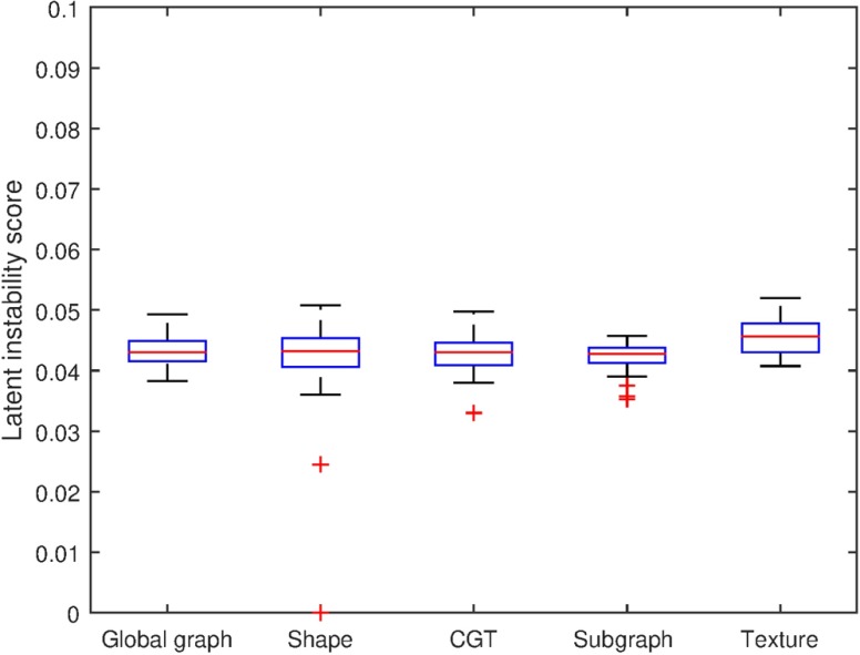
All feature families across all cohorts exhibited low LI scores. No feature family in any unstandardized dataset had a mean LI score higher than 0.0522 as seen in Table 3 and Fig. 3, indicating just a 5.22% chance of a feature being significantly different in a random split. These low LI scores were indicative of low intradataset feature instability. This suggests that within the same dataset, the features do not tend to vary considerably.
Table 3.
Mean and standard deviation of LI score by cohort and feature family.
| Site | Graph | Shape | CGT | Subgraph | Texture |
|---|---|---|---|---|---|
|
|
|
|
|
|
|
Note: The bold values represent the most stable and least stable feature families amongst the and cohorts.
Fig. 3.
Distribution of LI results by feature family.
4.2. Preparation-Induced Instability to Evaluate Feature Robustness Across Cohorts and Sites
To evaluate the effect of CN on feature value calculation and to investigate the role that CN plays in reduction of interdataset feature instability, we compared the number of feature distributions that were significantly different across datasets before and after normalization. We compared the mean preparation-induced instability score () for each family of features shown in Table 4 and Fig. 4 to the mean latent instability score () for that feature family. is the mean of the PI scores of all the features in a family and is the mean of a family’s LI across .
Table 4.
Mean and standard deviation of PI score in nonrecurrence Gleason 7 images of (top row) and (middle row) and in 34 images of across three scanners (bottom row).
| Dataset | Graph | Shape | CGT | Subgraph | Texture |
|---|---|---|---|---|---|
Note: The bold values represent the most stable and least stable feature families in each experiment.
Fig. 4.
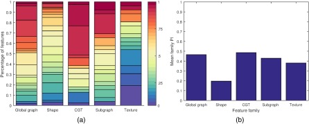
Summary of intra- and interdataset experiment results. (a) Feature family PI results by score frequency. Score indicates percentage of the 6 1000-iteration subsampled pairwise comparisons ( versus , versus , versus , versus , versus , versus ) in which the given feature was significantly different. Results plotted after grouping the 239 unique feature scores into 30 bins. (b) Average PI results by feature family computed as the mean score from all the features within a family.
Shape features were found to be most resilient while CGT features were the most unstable. Shape features were different among datasets times more often than would be expected without differences in slide preparation among datasets while CGT features were times more likely to be different.
CGT features measure the disorder of lumen orientation in neighborhoods of glands. Missed and erroneously segmented gland objects will have a larger effect on CGT features which compare glands to their neighbors while having less of an effect on shape measurements. This is consistent with the results. The families with high , graph, CGT, and subgraph, all depend on accurate gland detection. In contrast, the shape features are largely based off the shape of the lumen. These, therefore, appear to be less affected by segmentation errors. Texture features, which do not rely on segmentation, fall between the gland arrangement-dependent families and the shape family in terms of .
4.3. Cancerous and Noncancerous Region Classification to Determine Effect of Unstable Feature Families on Independent Validation
As seen in Table 5, the more unstable feature families, graph, CGT, and subgraph were significantly more accurate in intrasite classification than in the intersite task (, , and ). Shape, the most stable feature family, was the only feature family to perform equally well in intra- and intersite classification by AUC (, , ) with slightly higher accuracy in the intersite task (, , ). The performance drop of the more unstable features in independent validation and the consistency of the less unstable features suggests that feature instability affects the model’s generalizability.
Table 5.
Mean and standard deviation of AUC and accuracy of QH features in distinguishing tumor from benign regions over 100 iterations of a random forest classifier using Wilcoxon rank-sum test for feature selection at the confidence level. Intrasite classification performed using threefold cross validation, intersite classification performed using independent validation. Reported as average of and results. No texture features were predictive, and the family is therefore not represented here.
| Graph | Shape | CGT | Subgraph | All families | |
|---|---|---|---|---|---|
| Intrasite AUC | |||||
| Intersite AUC | |||||
| -Value | 0.88 | 0.29 | |||
| Intrasite accuracy | |||||
| Intersite accuracy | |||||
| -Value | 0.01 |
4.4. Evaluating Effect of Scanner Variation on Feature Stability
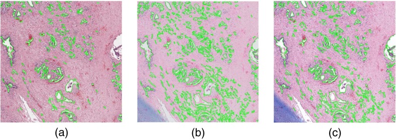
As seen in Table 4, automated segmentations of the same 34 slides scanned on three different scanners produced features which were less unstable in three families (global graph, CGT, and subgraph) and more unstable in one family (shape). The Haralick texture features were extremely unstable across scanners with a mean PI of 0.620 compared to 0.438 across . Notably, all the images used in the PI calculation were digitized using an Aperio scanner including and which were digitized on the exact same scanner. The scanner used appears to have a large effect on the texture features, which are dependent on color and contrast changes induced in the digitized slide images. It is possible the instability measurements of are affected by the Aperio scanner which in turn may explain the variation in the PI of the texture features between the two experiments. Figure 5 shows these variations as well as an example of the blue annotations added onto the slides by another group; however, features were extracted from regions entirely inside the blue contour.
Fig. 5.
A patient scanned on the (a) Aperio, (b) Phillips, and (c) Ventana scanners. The blue marker annotations were added between scans of the patient and were outside the region considered for feature analysis and thus did not affect feature values.
The lower instability of the global graph, CGT, and subgraph families in the experiment is not unexpected. While vary in sectioning, mounting, and staining procedures in addition to scanning equipment, only vary in digitization hardware. It is intuitive that datasets separated only by the scanner used would be more stable than datasets prepared by entirely different laboratories. However, the large increase in shape feature PI mean and standard deviation ( to ) is somewhat surprising as the shape features were the most stable feature family by a large margin in the experiment. Figure 6 shows that in some regions of interest, the automated segmentation performance varies greatly across scanners, though we did not undertake a quantitative assessment of the degree of segmentation variation. The very large standard deviation in shape feature PI as well as the instability variation among feature families suggests that some features are highly vulnerable to intersite variation while others are more robust.
Fig. 6.
Region of interest of a slide scanned on (a) Aperio, (b) Phillips, and (c) Ventana scanners with automated gland segmentation results overlaid. It is clear that the automated segmentation performed much worse on the Phillips scanner in this specific region.
4.5. Evaluating Effect of Color Normalization on Feature Stability
The PI and LI experiments were repeated using color normalized versions of the images of to study the effects of CN on feature stability. Images were standardized to a template image, thereby creating normalized datasets (see Fig. 7). The template image was chosen as one of the images where the automated segmentation algorithm was able to accurately extract the gland boundaries. An example of how the feature values may change before and after normalization is shown in Fig. 8.
Fig. 7.
Illustration of the experiment performed to evaluate the effect of CN on feature stability. (a) Source image to be normalized, (b) template image, and (c) resulting color transformed image. (d) Color histograms of pre-CN image (a) in solid lines and post-CN image (c) in dashed lines.
Fig. 8.
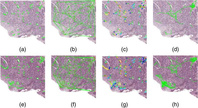
Segmentation and feature visualization on image (a–d) prenormalization and (e–h) postnormalization. (a, e) Automated segmentation results. Automatically extracted features corresponding to (b, f) global gland graphs, (c, d) gland disorder, and (d, h) local gland graphs.
The goal of the CN experiments was to quantify how CN affected the number of unstable features. A decrease in feature family PI or LI after normalization would suggest that the process of CN was playing a role in reducing feature instability across or within sites. Our results suggest that CN had no effect on overall feature stability. The largest change in PI between original and normalized data was a change of 0.019 in the subgraph features with CN actually increasing intersite instability in four of the five feature families (see Table 4). The largest change in LI was in the graph features which had an increase in mean LI of 0.003, representing a 0.3% point increase in intrasite instability.
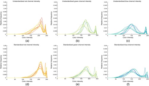
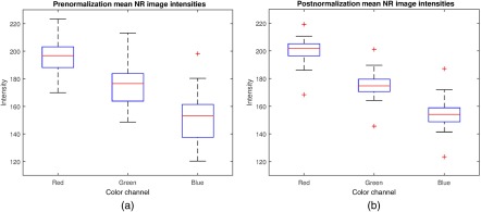
CN had a noticeable effect on the distribution of RGB values in the datasets. The histograms of eight images before and after normalization are shown in Fig. 9. After normalization, the histograms of each color channel were better aligned and had a more similar distribution. Notably, the chosen color standardization method18 does not operate in the RGB space. Hence the changes in the histograms are merely byproducts of the normalization of distributions in the color space. Figure 10 shows that the spread of RGB values across was reduced after normalization.
Fig. 9.
Histograms of color channel intensity distributions for eight images (a–c) before and (d–f) after normalization. (a) Red, (b) green, and (c) blue channel intensity distributions in prenormalization images. (d) Red (e) green, and (f) blue channel intensity distributions in postnormalization images.
Fig. 10.
Boxplots of the mean color channel intensities from each image in and (a) before normalization and (b) after normalization.
The results of the CN experiments also reveal that factors other than color appear to have played a large part in altering segmentation success and hence the resulting feature values. The chosen CN scheme is useful for this application because it attempts to normalize stain concentrations across images. Clearly the results of our experiments with CN will need to be validated via other CN schemes.
5. Concluding Remarks
In this paper, we presented a method for quantifying instability of features across multiple datasets and employed this method to determine stability in five feature families across four prostate cancer datasets with known variations due to staining, preparation, and scanning platforms. We introduced two new indices for quantifying feature instability and used them to identify which features previously shown to be predictive of cancer presence are most robust and stable. We found that all feature families exhibit differences among datasets from different institutions at a rate nearly 5 to 12 times what would be expected based on random chance. Although shape features were most resilient across datasets, all feature families exhibited sensitivity to staining and scanning procedure variations and the shape features themselves were especially vulnerable to scanner variation. With intra- and intersite classification, we have demonstrated that feature instability affects classifier performance and shown that a feature family’s mean PI may indicate the degree to which the accuracy of those features may degrade with site variability. We have demonstrated that while CN can definitely affect the feature values and their stability, CN alone cannot solve the problem of interdataset feature instability. We found that the number of features different among datasets can change after CN, but in our case this did not resolve feature instability. Limitations to this study include that we did not consider other sources of variation that might be affecting the stability of the feature values, e.g., variations in segmentation. While we qualitatively observed that the automated gland segmentations varied among different scanners, we did not quantitatively determine the extent or cause of this variation. We did not examine how these instability scores may vary when using data from other sites or how sensitive our scores were to the specific tissue images used to calculate them. Additionally, we only considered one CN scheme in this work and the results obtained need to be validated in conjunction with other CN methods. We have not investigated how stability information may be incorporated in feature selection or classifier construction and our use case was confined to a specific application involving cancer detection on prostate histopathology images. In future work, we will seek to look at the trade-off between feature discriminability and stability more comprehensively and in the context of other use cases. This framework for quantifying feature instability may be useful in designing and developing future digital pathology-based computer-aided diagnostic algorithms which will need robust and discriminating features in order to be generalizable and consistent across sites.
Acknowledgments
Research reported in this publication was supported by the National Cancer Institute of the National Institutes of Health under award numbers (R21CA167811-01, R21CA179327-01, R21CA195152-01, U24CA199374-01, and K01ES026841), National Institute of Diabetes and Digestive and Kidney Diseases (R01DK098503-02), DOD Prostate Cancer Synergistic Idea Development Award (PC120857), DOD Lung Cancer Idea Development New Investigator Award (LC130463), DOD Prostate Cancer Idea Development Award, Ohio Third Frontier Technology development Grant, CTSC Coulter Annual Pilot Grant, Case Comprehensive Cancer Center Pilot Grant, VelaSano Grant from the Cleveland Clinic, Wallace H. Coulter Foundation Program in the Department of Biomedical Engineering at Case Western Reserve University. The content is solely the responsibility of the authors and does not necessarily represent the official views of the National Institutes of Health.
Biography
Biographies for the authors are not available.
References
- 1.Xu J., et al. , “Stacked sparse autoencoder (SSAE) for nuclei detection on breast cancer histopathology images,” IEEE Trans. Med. Imaging 35(1), 119–130 (2016). 10.1109/TMI.2015.2458702 [DOI] [PMC free article] [PubMed] [Google Scholar]
- 2.Ginsburg S., et al. , “Feature importance in nonlinear embeddings (FINE): applications in digital pathology,” IEEE Trans. Med. Imaging 35(1), 76–88 (2016). [DOI] [PubMed] [Google Scholar]
- 3.Sridhar A., Doyle S., Madabhushi A., “Content-based image retrieval of digitized histopathology in boosted spectrally embedded spaces,” J. Pathol. Inf. 6, 41 (2015). 10.4103/2153-3539.159441 [DOI] [PMC free article] [PubMed] [Google Scholar]
- 4.Ali S., et al. , “Selective invocation of shape priors for deformable segmentation and morphologic classification of prostate cancer tissue microarrays,” Comput. Med. Imaging Graphics 41, 3–13 (2015). 10.1016/j.compmedimag.2014.11.001 [DOI] [PMC free article] [PubMed] [Google Scholar]
- 5.Lee G., et al. , “Supervised multi-view canonical correlation analysis (sMVCCA): integrating histologic and proteomic features for predicting recurrent prostate cancer,” IEEE Trans. Med. Imaging 34, 284–297 (2015). 10.1109/TMI.2014.2355175 [DOI] [PubMed] [Google Scholar]
- 6.Lee G., et al. , “Co-occurring gland angularity in localized subgraphs: predicting biochemical recurrence in intermediate-risk prostate cancer patients,” PLoS One 9, e97954 (2014). 10.1371/journal.pone.0097954 [DOI] [PMC free article] [PubMed] [Google Scholar]
- 7.Cruz-Roa A., et al. , “A deep learning architecture for image representation, visual interpretability and automated basal-cell carcinoma cancer detection,” Lect. Notes Comput. Sci. 8150, 403–410 (2013). 10.1007/978-3-642-40763-5 [DOI] [PubMed] [Google Scholar]
- 8.Lee G., et al. , “Cell orientation entropy (COrE): predicting biochemical recurrence from prostate cancer tissue microarrays,” Lect. Notes Comput. Sci. 8151, 396–403 (2013). 10.1007/978-3-642-40760-4 [DOI] [PubMed] [Google Scholar]
- 9.Lewis J. S., et al. , “A quantitative histomorphometric classifier (QuHbIC) identifies aggressive versus indolent p16-positive oropharyngeal squamous cell carcinoma,” Am. J. Surg. Pathol. 38, 128–137 (2014). 10.1097/PAS.0000000000000086 [DOI] [PMC free article] [PubMed] [Google Scholar]
- 10.Sparks R., Madabhushi A., “Explicit shape descriptors: novel morphologic features for histopathology classification,” Med. Image Anal. 17, 997–1009 (2013). 10.1016/j.media.2013.06.002 [DOI] [PMC free article] [PubMed] [Google Scholar]
- 11.Sparks R., Madabhushi A., “Statistical shape model for manifold regularization: Gleason grading of prostate histology,” Comput. Vision Image Understanding 117, 1138–1146 (2013). 10.1016/j.cviu.2012.11.011 [DOI] [PMC free article] [PubMed] [Google Scholar]
- 12.Basavanhally A., et al. , “Multi-field-of-view framework for distinguishing tumor grade in ER+ breast cancer from entire histopathology slides,” IEEE Trans. Biomed. Eng. 60, 2089–2099 (2013). 10.1109/TBME.2013.2245129 [DOI] [PMC free article] [PubMed] [Google Scholar]
- 13.Lyon H., et al. , “Standardization of reagents and methods used in cytological and histological practice with emphasis on dyes, stains and chromogenic reagents,” Histochem. J. 26(7), 533–544 (1994). 10.1007/BF00158587 [DOI] [PubMed] [Google Scholar]
- 14.Oliver J. A., et al. , “Variability of image features computed from conventional and respiratory-gated PET/CT images of lung cancer,” Transl. Oncol. 8(6), 524–534 (2015). 10.1016/j.tranon.2015.11.013 [DOI] [PMC free article] [PubMed] [Google Scholar]
- 15.Fave X., et al. , “Can radiomics features be reproducibly measured from CBCT images for patients with non-small cell lung cancer?” Med. Phys. 42(12), 6784–6797 (2015). 10.1118/1.4934826 [DOI] [PMC free article] [PubMed] [Google Scholar]
- 16.Nyflot M. J., et al. , “Quantitative radiomics: impact of stochastic effects on textural feature analysis implies the need for standards,” J. Med. Imaging 2(4), 041002 (2015). 10.1117/1.JMI.2.4.041002 [DOI] [PMC free article] [PubMed] [Google Scholar]
- 17.Leijenaar R. T., et al. , “Stability of FDG-PET radiomics features: an integrated analysis of test-retest and inter-observer variability,” Acta Oncol. 52(7), 1391–1397 (2013). 10.3109/0284186X.2013.812798 [DOI] [PMC free article] [PubMed] [Google Scholar]
- 18.Khan A. M., et al. , “A nonlinear mapping approach to stain normalization in digital histopathology images using image-specific color deconvolution,” IEEE Trans. Biomed. Eng. 61(6), 1729–1738 (2014). 10.1109/TBME.2014.2303294 [DOI] [PubMed] [Google Scholar]
- 19.Reinhard E., et al. , “Color transfer between images,” IEEE Comput. Graphics Appl. 21, 34–41 (2001). 10.1109/38.946629 [DOI] [Google Scholar]
- 20.Macenko M., et al. , “A method for normalizing histology slides for quantitative analysis,” in IEEE Int. Symp. on Biomedical Imaging: From Nano to Macro (ISBI ’09), pp. 1107–1110 (2009). [Google Scholar]
- 21.Kothari S., et al. , “Automatic batch-invariant color segmentation of histological cancer images,” in IEEE Int. Symp. on Biomedical Imaging: From Nano to Macro (ISBI ‘11), pp. 657–660 (2011). 10.1109/ISBI.2011.5872492 [DOI] [PMC free article] [PubMed] [Google Scholar]
- 22.Ghaznavi F., et al. , “Digital imaging in pathology: whole-slide imaging and beyond,” Annu. Rev. Pathol. Mech. Dis. 8, 331–359 (2013). 10.1146/annurev-pathol-011811-120902 [DOI] [PubMed] [Google Scholar]
- 23.Doyle S., et al. , “Cascaded discrimination of normal, abnormal, and confounder classes in histopathology: Gleason grading of prostate cancer,” BMC Bioinf. 13, 282 (2012). 10.1186/1471-2105-13-282 [DOI] [PMC free article] [PubMed] [Google Scholar]
- 24.Hipp J., et al. , “Integration of architectural and cytologic driven image algorithms for prostate adenocarcinoma identification,” Anal. Cell. Pathol. 35(4), 251–265 (2012). 10.3233/ACP-2012-0054 [DOI] [PMC free article] [PubMed] [Google Scholar]
- 25.Yu E., et al. , “Detection of prostate cancer on histopathology using color fractals and probabilistic pairwise Markov models,” in IEEE Int. Conf. of Engineering in Medicine and Biology Society (EMBS ‘11), pp. 3427–3430 (2011). 10.1109/IEMBS.2011.6090927 [DOI] [PubMed] [Google Scholar]
- 26.Golugula A., et al. , “Supervised regularized canonical correlation analysis: integrating histologic and proteomic measurements for predicting biochemical recurrence following prostate surgery,” BMC Bioinf. 12, 483 (2011). 10.1186/1471-2105-12-483 [DOI] [PMC free article] [PubMed] [Google Scholar]
- 27.Madabhushi A., et al. , “Computer-aided prognosis: predicting patient and disease outcome via quantitative fusion of multi-scale, multi-modal data,” Comput. Med. Imaging Graphics 35, 506–514 (2011). 10.1016/j.compmedimag.2011.01.008 [DOI] [PubMed] [Google Scholar]
- 28.Doyle S., et al. , “A boosted Bayesian multiresolution classifier for prostate cancer detection from digitized needle biopsies,” IEEE Trans. Biomed. Eng. 59, 1205–1218 (2012). 10.1109/TBME.2010.2053540 [DOI] [PubMed] [Google Scholar]
- 29.Monaco J. P., et al. , “High-throughput detection of prostate cancer in histological sections using probabilistic pairwise Markov models,” Med. Image Anal. 14, 617–629 (2010). 10.1016/j.media.2010.04.007 [DOI] [PMC free article] [PubMed] [Google Scholar]
- 30.Breiman L., “Random forests,” Mach. Learn. 45(1), 5–32 (2001). 10.1023/A:1010933404324 [DOI] [Google Scholar]
- 31.Pizer S. M., et al. , “Adaptive histogram equalization and its variations,” Comput. Vision Graphics Image Process. 39(3), 355–368 (1987). 10.1016/S0734-189X(87)80186-X [DOI] [Google Scholar]
- 32.Nguyen K., et al. , “Structure and context in prostatic gland segmentation and classification,” Lect. Notes Comput. Sci. 7510, 115–123 (2012). 10.1007/978-3-642-33415-3 [DOI] [PubMed] [Google Scholar]
- 33.Ginsburg S. B., et al. , “Novel PCA-VIP scheme for ranking MRI protocols and identifying computer-extracted MRI measurements associated with central gland and peripheral zone prostate tumors,” J. Magn. Reson. Imaging 41, 1383–1393 (2015). 10.1002/jmri.v41.5 [DOI] [PMC free article] [PubMed] [Google Scholar]
- 34.Haralick R. M., Shanmugam K., Dinstein I. H., “Textural features for image classification,” IEEE Trans. Syst, Man Cybern. 3(6), 610–621 (1973). 10.1109/TSMC.1973.4309314 [DOI] [Google Scholar]
- 35.National Cancer Institute, “Home—The Cancer Genome Atlas-Cancer Genome-TCGA,” 2016, http://cancergenome.nih.gov/.


