eLife logoLink to eLife
. 2016 Oct 3;5:e20252. doi: 10.7554/eLife.20252

Sparse activity of identified dentate granule cells during spatial exploration

Maria Diamantaki 1,2, Markus Frey 1, Philipp Berens 1,3,4, Patricia Preston-Ferrer 1,*, Andrea Burgalossi 1,*
Editor: Karel Svoboda5
PMCID: PMC5077296  PMID: 27692065

Abstract

In the dentate gyrus – a key component of spatial memory circuits – granule cells (GCs) are known to be morphologically diverse and to display heterogeneous activity profiles during behavior. To resolve structure–function relationships, we juxtacellularly recorded and labeled single GCs in freely moving rats. We found that the vast majority of neurons were silent during exploration. Most active GCs displayed a characteristic spike waveform, fired at low rates and showed spatial activity. Primary dendritic parameters were sufficient for classifying neurons as active or silent with high accuracy. Our data thus support a sparse coding scheme in the dentate gyrus and provide a possible link between structural and functional heterogeneity among the GC population.

DOI: http://dx.doi.org/10.7554/eLife.20252.001

Research Organism: Rat

Introduction

Sparse activity is a hallmark feature of cortical and hippocampal function (Treves and Rolls, 1994; Olshausen and Field, 2004; Wolfe et al., 2010; Barth and Poulet, 2012; Spanne and Jörntell, 2015). In neocortical circuits, sparse representations are thought to be crucial for optimal encoding of sensory stimuli (Brecht et al., 2004; Huber et al., 2008; Li et al., 2009; Rochefort et al., 2009). Similarly in hippocampal circuits, the skewed distribution of population firing activity indicates that a preconfigured, highly active minority of neurons dominates information coding (Mizuseki and Buzsáki, 2013; Buzsaki and Mizuseki, 2014). Whether and how this highly active population is structurally or molecularly different from the majority of neurons remains to be established. The dentate gyrus (DG) is among the most sparse networks known to date. Extracellular recordings in foraging rodents have in fact revealed that only a tiny minority of principal neurons – putative granule cells (GCs) – is active during behavior, while the rest are silent (Jung and McNaughton, 1993; Skaggs et al., 1996; Neunuebel and Knierim, 2012). Although several structure–function schemes have been proposed (Leutgeb et al., 2007; Alme et al., 2010; Lisman, 2011; Neunuebel and Knierim, 2014), the cellular identity of active and silent neurons has remained largely unexplored.

Here, we addressed this issue by employing juxtacellular recording and labeling procedures in freely moving rats (Tang et al., 2014a). An advantage of this technique over conventional extracellular methods is that neurons can be identified irrespective of their spiking activity; thus, both silent and active cells can be sampled during free behavior (i.e. under intact sensory, motor and vestibular inputs), which enables the analysis of sparsely active networks (Hromádka et al., 2008; O'Connor et al., 2010; Herfst et al., 2012; Burgalossi et al., 2014). We provide a quantitative assessment of sparse activity in the rat’s DG and show that a subset of mature GCs with complex dendritic trees contributes to the active pool.

Results

In a first set of experiments, we aimed to explore electrophysiological signatures of GC activity. To this end, we juxtacellularly recorded and labeled spontaneously active neurons in the rat DG in-vivo. From these recordings, we observed that active GCs displayed a characteristic spike waveform, as shown in the representative example in Figure 1A–C. Here, a spontaneously active GC was recorded and identified in a head-fixed awake rat. This neuron displayed morphological features of mature GCs (see Materials and methods and Figure 1A) and discharged sparsely during the awake state (average firing rate=0.49 Hz; Figure 1B). Notably, spikes from this neuron displayed a ‘shoulder’ following the positive peak of the juxtacellular spike, which was best evident as a local maximum in the first derivative of the juxtacellular voltage trace (Figure 1C). Altogether, we recorded and identified 47 active neurons during urethane theta-oscillations (n=19), awake head-fixation (n=4) and free-behavior (n=24) (Figure 1D). In these recordings, the presence of spike-shoulders was determined by the intersection between the spike trace and its moving average during the repolarization phase of the spike (see Figure 1—figure supplement 1). Irrespective of the recording condition (i.e. anesthetized versus awake), we found that all neurons displaying spike-shoulders were located within the GC layer (n=17; with the exception of one excitatory neuron just below the GC layer; see Figure 1D,E and Materials and methods) and corresponded to morphologically mature GCs (see criteria in Materials and methods; n=15 cases where morphology could be assessed). In CA3c (n=7), fast-spiking (n=10) and hilar (n=17) neurons, spike-shoulders were not identified (Figure 1F). In most cases spike-shoulders from GCs were already apparent in the average spike waveform (Figure 1C,E and Figure 1—figure supplement 1A) and resulted in a relatively long duration of the juxtacellular spike signal (Figure 1G). Furthermore, recordings could be assigned with high accuracy to the GC class based solely on the average spike waveforms (~89%; cross-validated; see Materials and methods for details), thus providing additional evidence for a correlation between spike-shoulders and GC identity.

Figure 1. Spike waveform features of identified granule cells.

(A) Reconstruction of the somatodendritic morphology of a morphologically mature GC recorded in an awake, head-fixed animal. (B) Representative raw (top) and high-pass filtered (bottom) spike trace recorded under head-fixation from the cell shown in (A). (C) Average spike waveform (black) of the cell shown in (A). Note the presence of the shoulder (black arrowhead) on the spike waveform and the corresponding peak (white arrowhead) in the first derivative below (blue, dV/dt). The right panel shows a magnification of the inset on the left. The ‘shoulder width’ measured at half-maximum of the average spike waveform’s first derivative is illustrated by the double-headed arrow. The first derivative is scaled up for illustration purposes. (D) Schematic outline of the dentate gyrus showing the somatic location of all active neurons recorded and identified juxtacellularly (n=47 neurons: GCs, n=21; hilar cells, n=17; CA3c cells, n=7; and fast-spiking cells, n=2; see details in Materials and methods). Recordings where spike-shoulders (‘AP-shoulders’) were or were not detected are indicated as black or grey dots, respectively. The asterisk indicates the neuron located below the GC layer, where shoulders were also identified (see Materials and methods for details). (E) Representative normalized average spike waveforms (black) of four identified GCs with their corresponding first derivatives (blue). Black arrowheads indicate the spike-shoulder and white arrowheads the local peak in the first derivatives. First derivatives are scaled up for illustration purposes. The location of these cells within the GC layer is indicated by the corresponding numbers in (D). (F) Representative normalized average spike waveforms (black) of an identified CA3c cell, an identified fast-spiking cell (FS) and an identified hilar cell (Hil) with their corresponding first derivatives (blue). Note the absence of shoulders in the spike waveforms and first derivatives. First derivatives are scaled up for illustration purposes. (G) Correlation between spike width and ‘shoulder width’ for all identified GCs (n=21, see panel D). Regression line (black), Pearson’s correlation coefficient (r) and p-value are indicated. AP=action potential; Hil=hilus; GCL=granule cell layer; ML=molecular layer.

DOI: http://dx.doi.org/10.7554/eLife.20252.002

Figure 1.

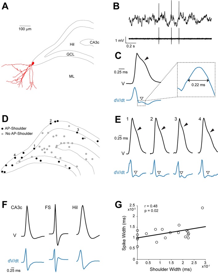
Figure 1—figure supplement 1. Detection of spike-shoulders.

Figure 1—figure supplement 1.

(A) Representative average spike waveform of an identified GC (Id 98), showing how the moving-average approach was used to detect the presence of spike-shoulders. The moving average (red dotted trace) was used to smooth high-frequency fluctuations in the spike trace (black) and to capture the underlying slow trends. The spike trace in the repolarization phase was compared to its time-lagged average and slower changes (shoulders) were detected as intersections between them. The right panel shows a close-up magnification of the intersection (indicated by a red circle) between spike voltage trace and its moving average. (B) Variability of spike-shoulder prominence (quantified as the half-width of the local maximum on the first derivative of the spike trace; see Materials and methods) and location relative to the spike peak (quantified as the time difference between the spike-peak and the intersection with the moving average, as in A) for identified (Id.; n=6) and classified GCs (Put.; n=18) recorded in freely moving rats. Error bars indicate SEM. The variability of spike shoulders was not significantly different between identified and classified GCs (p-values are indicated; Mann-Whitney test).

Next, we performed juxtacellular recordings from single DG neurons while rats explored an open-field environment or an elevated ‘O’ maze. Of 190 juxtacellular recordings established in the GC layer, 163 were from silent neurons (see Materials and methods and Figure 2). Figure 2A–D shows two examples of identified silent GCs, recorded during free behavior. Both neurons displayed morphological features of mature GCs (Figure 2A,C) and did not fire during exploration (Figure 2B,D). Spiking was readily induced by current injection (Figure 2E), which was used in a subset of cases to label the neurons at the end of the recording session (see Materials and methods; Pinault, 1996; Herfst et al., 2012; Tang et al., 2014a).

Figure 2. Silent granule cells during spatial exploration.

Figure 2.

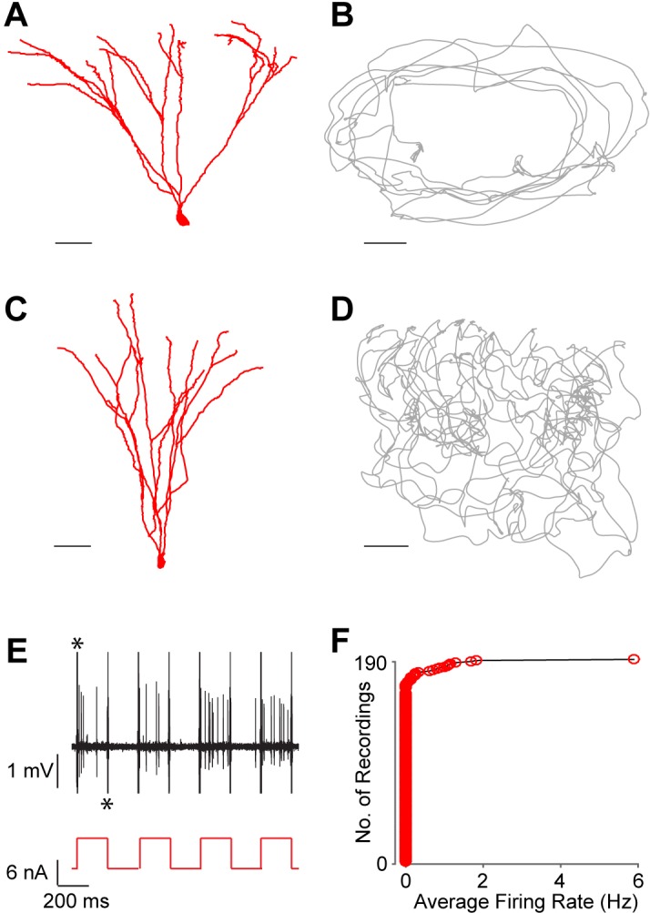
(A and C) Reconstruction of the dendritic morphology of two silent, morphologically mature GCs recorded during freely moving behavior (cell ids 924 and 991, respectively). Scale bars=50 µm. (B and D) Trajectory of a rat (grey) running on an O-shaped arena (B) or on an open-fieldarena (D). The two recordings correspond to the neurons in (A and C), respectively. Scale bars=10 cm. (E) Unlike extracellular recordings, juxtacellular sampling is not biased towards active cells, as silent neurons can also be recorded and their presence confirmed by current injection. This is shown here for the silent cell in (C): action potential firing (black, top) induced by squared pulses of injected current (red, bottom). These pulses were delivered at the end of the freely moving recording session to confirm the presence of the silent celland to label the cell (C). Asterisks indicate stimulation artifacts (truncated for display purposes). (F) Cumulative plot showing the firing-rate distribution within the GC layer. Each red circle represents one neuron, sampled juxtacellularly within the GC layer (see Materials and methods for details). Note the large proportion of silent neurons (163 out of 190) compared to that of active cells; this is likely to be an underestimate of the true silent proportion (see Results and Materials and methods for details).

DOI: http://dx.doi.org/10.7554/eLife.20252.004

Active GCs were thus very sparse and accounted for only ~14% (27 out of 190) of all neurons sampled within the GC layer (Figure 2F; we note that this is likely to represent an overestimate, since silent juxtacellular ‘hits’ were often discarded; see Materials and methods). Nine spontaneously active GCs were successfully labeled and identified in freely moving animals; consistent with previous observations (Jung and McNaughton, 1993; Skaggs et al., 1996), the sharpest spatial activity was observed within the subset of neurons displaying highest firing rates (>1 Hz); two of these neurons are shown in Figure 3A–H. The first morphologically mature GC (Figure 3A) was recorded in an open square maze and displayed a single firing field (Figure 3B). A large fraction of spikes (Figure 3C) occurred within bursts (Figure 3D; see also Pernía-Andrade and Jonas, 2014) and was rhythmically entrained by local field potential (LFP) theta oscillations (4–12Hz; Figure 3E). The second neuron was also a mature GC (Figure 3F). It was recorded while the rat explored an ‘O’ maze, and a single firing field was observed (Figure 3G). Spikes of this identified neuron also displayed shoulders (Figure 3H).

Figure 3. Spatial and temporal firing properties of identified active granule cells.

(A) Left, single-plane confocal image showing a morphologically mature GC (cell id 103) located in the infrapyramidal blade, recorded and labeled in a freely moving animal. Right, reconstruction of dendritic (red) and axonal (blue) morphologies; only the axon extending within the hilus (Hil) is shown. Close anatomical proximity (< 1 µm; compatible with putative synaptic contacts) was observed between mossy boutons and large hilar neurons (4 out of 13 analyzed boutons; not shown), suggesting that hilar neurons might integrate spatial signals from upstream GCs. Scale bars=50 μm. GCL=granule cell layer; ML=molecular layer. (B) Spike-trajectory plot (top) and rate map (bottom) for the neuron shown in (A), recorded in a square arena. Scale bar=10 cm. (C) Representative high-pass filtered spike trace, recorded during free behavior from the neuron in (A). (D) Interspike interval (ISI) distribution for the neuron in (A). Note the early peak (arrowhead) representing short ISI within bursts. (E) Spike-autocorrelogram for the neuron in (A). Note the prominent rhythmicity in the theta-frequency range (~8 Hz during awake behavior). (F) Reconstruction of the dendritic morphology of an active morphologically mature GC (cell id 104) recorded during freely moving behavior. Scale bar=50 µm. (G) Spike-trajectory plot (top) and rate map (bottom) for the neuron shown in (F) recorded on an O-shaped linear arena. Scale bar=10 cm. (H) Normalized average spike waveform (black) of the neuron shown in (F), with corresponding first derivative (blue). Black arrowhead indicates the spike-shoulder and white arrowhead the local peak in the first derivative. The first derivative is scaled up for illustration purposes. (I) Fluorescence micrograph showing a histologically verified electrode track (red dotted line) and recordings site (dotted circle), which was localized to the superficial portion of the GC layer (end of the track). Note the presence of small cell debris at the labeling site (dotted circle). (J) Spike-trajectory plot (top) and rate map (bottom) for the recording location shown in (I) (putative GC recording, cell id 80) during exploration of a square open arena. Scale bar= 10 cm. (K) Same as in (H), but for the putative GC recording in (I).

DOI: http://dx.doi.org/10.7554/eLife.20252.005

Figure 3.

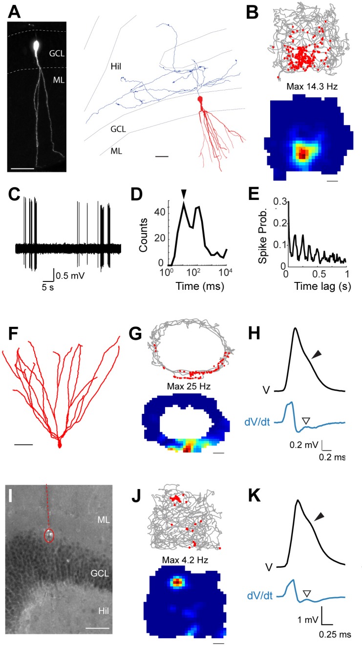
Figure 3—figure supplement 1. Spatial firing activity of identified and putative GCs.

Figure 3—figure supplement 1.

(A) Spike-trajectory plots (left) and rate maps (middle) for the identified GCs which were classified as spatially modulated (see Materials and methods for details). Cell id and maximal firing rates are indicated. In the right panels, firing fields are outlined as grey areas (see Materials and methods). The total size of the firing fields (expressed in number of pixels) is indicated. For cell id 102, the multiple firing fields might result from suboptimal spatial coverage, as indicated by the close-up magnification on a single-pass at the upper-left corner of the maze. The corresponding high-pass filtered juxtacellular spike trace is indicated. (B) Same as (A), but for ‘putative’ GCs.

Given the correlation between spike-shoulders and GC identity (see Figure 1), we sought to take advantage of this waveform signature (together with the anatomical location of the electrode track in the GC layer, see Materials and methods) for classifying unidentified juxtacellular recordings obtained in freely moving animals. An example of a classified GC recording is shown in Figure 3I–K. In this recording, cell identification by juxtacellular labeling failed, but the recording site could be localized to the GC layer (see Figure 3I and Materials and methods). This neuron fired only a few spikes during behavior, which tended to cluster at a single spatial location (Figure 3J). Spikes fired by this neuron displayed prominent shoulders (Figure 3K), a strong correlate of GC identity (Figure 1). Altogether, we recorded 27 active GCs (9 identified and 18 classified) during spatial exploration. We note that since most but not all identified active GCs displayed spike-shoulders (18 out of 21; ~86%, Figure 1D), a fraction of GC recordings (~14%) is likely to be misclassified as false-negative in our dataset. In line with the examples shown in Figure 3, in the majority of cases firing occurred at single spatial locations (8 out of 11 recordings; Figure 3—figure supplement 1; see details in Materials and methods), suggesting that these spatial firing patterns are likely to arise from the mature GC population (Danielson et al., 2016).

Next, we explored whether the heterogeneity of GC activity during behavior might relate to the morphological properties of the neurons. To this end, we first reconstructed the somato-dendritic compartment of seven silent and six active GCs (all of which were classified as morphologically mature; see Figure 4A,B, Figure 4—figure supplement 1 and criteria in Materials and methods), which were selected for the morphological analysis on the basis of their high-quality filling (see Figure 4—figure supplement 2B–D and Materials and methods). We then trained a logistic regression classifier enforcing different levels of sparsity in the weights with different primary morphological metrics (total dendritic length, total length of dendritic branch orders, number of primary dendrites and number of dendritic endings) as features (Figure 4C and Figure 4—source data 1). The classifier was able to distinguish active and silent cells with good accuracy independent of the enforced level of sparsity (leave-one-out cross-validation accuracy ~85%, 11 out of 13 cells classified correctly). This classification accuracy was significantly higher than chance (p=0.03, permutation test, 500 runs, see Materials and methods). For lower levels of sparsity, the classifier used a more distributed weight profile, whereas for higher levels, the weight used was more concentrated on individual predictors (Figure 4D). Overall, longer high-order dendrites (5 and 6 orders) were most predictive of active cells, whereas shorter low-order dendrites (2 and 3 orders) together with a higher number of primary dendrites were most predictive of silent cells (Figure 4D). Notably, the morphological differences between active and silent neurons (Figure 4A,B) were unlikely to have resulted from methodological or procedural biases (see Figure 4—figure supplement 2 and Materials and methods for more details). This indicates that in our dataset of identified neurons (n=13), dendritic architectures can be predictive of GC activity during behavior (see also Figure 4—source data 1).

Figure 4. Morphological analysis of identified active and silent granule cells.

(A) Somatodendritic reconstructions of silent (left, cell id 993) and active (right, cell id 102) GCs, recorded in freely moving rats. Dendritic branch orders 1–3 are indicated in black, while high-order branches (≥ 4) are indicated in red. Scale bar=50 µm. (B) Dendrograms for the cells in (A). The branch orders of the terminal dendritic tips are indicated. Color codes same as in (A). Scale bar=50 µm. (C) Box-plots comparing primary dendritic parameters (active GCs, n=6; silent GCs, n=7). Whiskers represent 1.5 IQR. Outliers are shown as crosses. (D) Weights of logistic regression classifier (mean ± SEM over cross-validation folds) used for classifying GCs as active or silent for different levels of sparseness (α=0.05 corresponds to dense weights, α=0.95 corresponds to sparse weights).

DOI: http://dx.doi.org/10.7554/eLife.20252.007

Figure 4—source code 1. Classification analysis.
Matlab script to load Figure 4—source data 1, run the logistic regression classification analysis on primary morphological features (Figure 4D), perform the shuffle analysis and run the control analysis with all morphological features.
DOI: 10.7554/eLife.20252.008
Figure 4—source data 1. Electrophysiological and morphological parameters of the identified GCs.
The table summarizes the main electrophysiological and morphological properties of the identified and reconstructed silent and active GCs (source data for Figure 4). Morphologies of the neurons are shown in Figure 4—figure supplement 1.
DOI: 10.7554/eLife.20252.009

Figure 4.

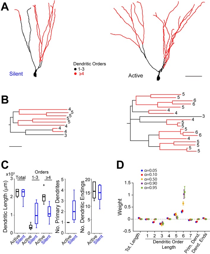
Figure 4—figure supplement 1. Morphological reconstructions of GCs recorded and labeled in freely moving rats.

Figure 4—figure supplement 1.

(A, B) Morphological reconstructions of silent (A) and active (B) GCs, recorded in freely moving rats. Dendritic branch orders 1–3 are indicated in black, while high-order branches (≥4) are indicated in red (same color-code as in Figure 4A). The insets show close-up magnifications of the soma and the proximal dendrites of each cell (first-order dendrites are in blue, second-order in green, third-order in orange and fourth-order in magenta). Scale bars=100 µm for the low magnification and 10 μm for the insets. Cell ids are indicated.

Figure 4—figure supplement 2. Distribution of recordings across animals and quantification of single-cell labeling quality.

Figure 4—figure supplement 2.

(A) Histogram showing the distribution of active (red) and silent recordings (blue) across animals (only recordings lasting > 60 s are included in the analysis; see Materials and methods). Identified recordings are indicated by the corresponding ids. Note that to ensure unequivocal cell identification, a low number of electrode penetrations and recordings were performed for each rat (average number of recordings per rat = 3.2 ± 2.7). In the animals with a relatively large number of recordings (> 5), either labeling was not attempted or cell identification could not be assured with certainty because of multiple consecutive electrode penetrations. We note that, given the relatively small number of observations for each rat, a dependency between rat identity and morphological properties cannot be rigorously tested and thus formally ruled out. (B) Representative micrographs of distal dendritic segments for an active and a silent neuron. Scale bars=10 µm. (C) Maximum gray scale values for distal dendritic compartments (top) and the ratio between distal and proximal dendrites (bottom) for active (n=6) and silent neurons (n=7). p-values are indicated (Mann-Whitney U test). See Materials and methods for details. (D) Distribution of terminal dendritic endings as a function of distance from the soma for active (n=6, red) and silent neurons (n=7, blue). Lines represent means, shadows represent SD. The distances of dendritic endings were not significantly different between active and silent neurons (Mann Whitney U Test, p-value is indicated).

Discussion

Sparse coding in the DG has been postulated to subserve ‘pattern separation’, a key function during memory processing (McNaughton and Morris, 1987; Leutgeb et al., 2007; Myers and Scharfman, 2009; Neunuebel and Knierim, 2014). Here we show that indeed the large majority of juxtacellularly sampled neurons within the GC layer are silent during exploration. The small fraction of active GCs (Figure 2F) displayed characteristic juxtacellular spike waveforms, characterized by the presence of ‘shoulders’ following the positive action potential peak (Figure 1C,E). Although, at present, we ignore the relative contributions of capacitive and/or ionic mechanisms to spike-shoulders, they served as a reliable correlate of GC identity. If such waveform signatures can also be resolved extracellularly – which remains to be demonstrated – they could be instrumental for future classification of tetrode-recorded DG units. We also provide direct anatomical evidence that morphologically mature GCs can display spatial firing, which in most cases occurred at single spatial locations (Figure 3—figure supplement 1). Although this is consistent with previous work (Leutgeb et al., 2007; Neunuebel and Knierim, 2012), the limited recording durations and spatial sampling prevent rigorous comparison with previous extracellular studies. Recordings in large open-field environments will be required to resolve whether different firing patterns (single versus multiple firing fields) are contributed by distinct cell types within the DG (Neunuebel and Knierim, 2012).

Previous work has demonstrated that cell intrinsic and synaptic mechanisms can be major determinants of single-cell activity in sparsely active networks (Crochet et al., 2011; Epsztein et al., 2011). Our data indicate that the dendritic architecture of mature GCs can be predictive of in-vivo spiking activity (Figure 4D), thus providing a possible structure–function scheme for active and silent neurons. We note, however, that in our limited dataset of identified GCs (n=13) structure–function relationships are subtle, as they derive from the combined analysis of multiple structural parameters (Figure 4D). Future work – possibly involving targeted manipulations of dendritic structures – will be required to resolve the causal contribution of GC dendritic architectures to spatial representations.

Materials and methods

Juxtacellular recordings

Experimental procedures for juxtacellular recordings, signal acquisition and processing, and animal tracking were essentially performed as recently described (Tang et al., 2014a; Diamantaki et al., 2016). The electrode solution contained standard Ringer solution: 135 mM NaCl, 5.4 mM KCl, 5 mM HEPES, 1.8 mM CaCl2 and 1 mM MgCl2 (pH is adjusted to 7.2). In a subset of recordings, neurobiotin (1.5–3%; Vector Laboratories, Burlingame, CA) or biocytin (1.5–3%; Sigma-Aldrich, St Louis, MO) was added to the electrode solution. Osmolarity was adjusted to 290-320 mOsm. Sample sizes were estimated on the basis of previously published data using similar procedures (Ray et al., 2014; Tang et al., 2014b; Tang et al., 2015).

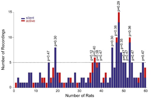
Juxtacellular recordings in anesthetized Wistar rats (n=11) were performed under ketamine/xylazine/urethane anesthesia, essentially as previously described (Klausberger et al., 2003; Ray et al., 2014). Juxtacellular recordings in awake, head-fixed Wistar rats (n=4) were performed as previously described (Houweling and Brecht, 2008; Doron et al., 2014; Tang et al., 2014a). Briefly, animals were pre-implanted with a metal post and a recording chamber under ketamine/xylazine anesthesia, and a craniotomy was performed at the coordinates for targeting the dorsal DG (3.5–4 mm posterior and 1.5–2 mm lateral from bregma). After a recovery period (~3–5 days), animals were slowly habituated to head-fixation. After successful habituation, and before juxtacellular recordings, mapping experiments with low resistance electrodes (0.5–1 MΩ) were performed to estimate the location of the DG precisely. Electrode penetrations were adjusted in order to target the DG blades and the crest. Juxtacellular recordings in freely moving Wistar rats (n=60) were performed as previously described (Tang et al., 2014a; Diamantaki et al., 2016). Implantation and mapping procedures were similar to those described above for the head-fixed preparation. After recovery from the surgery, animals were slowly habituated to the head-fixation and to collect chocolate/food pellets, as recently described (Diamantaki et al., 2016). Training and recording was performed in three types of arenas: a square maze (70 × 70 cm) with 25 cm high walls, a wall-less maze (55 × 65 cm) and an elevated, O-shaped, linear maze (70 × 50 cm, 14 cm wide path). All animals underwent the same training prior to the experiments (> 3 days, > 9 total sessions). 67 recordings from silent neurons in the O-shaped linear maze come from our previous work (Diamantaki et al., 2016), and 33 of these neurons were recorded during the first 3 days of exposure to a novel environment; as the fraction of active/silent neurons did not change significantly as a function of habituation (active/silent neurons during the first 3 days of habituation=9/42; active/silent neurons after > 3 days of habituation=18/121; p=0.48, Fisher’s Exact Test), these recordings were pooled and included in Figure 2F for estimating the proportion of active/silent neurons within the GC layer.

Juxtacellular labeling was performed by using standard labeling protocols (Pinault, 1996) and modified procedures, which consisted of rapidly breaking the dielectric membrane resistance with short (1–2 ms) ‘buzz-like’ current pulses (using the built-in buzz module of the ELC-X03 amplifier, NPI Electronic, Tamm, Germany), which provided rapid access to cell entrainment by juxtacellular current injection, i.e. 200 ms square current pulses, 1–10 nA (Pinault, 1996). At relatively high concentrations of neurobiotin or biocytin (i.e. 2.5–3%), short access to the cell’s interior was occasionally sufficient for recovering labeled neurons. The same labeling procedures were applied to active and silent neurons, which resulted in similar success rates of juxtacellular filling (see Results). Recordings (or portions of recordings) in which cellular damage was observed – e.g. spike-shape broadening, increase in firing rate accompanied by negative DC-shifts of the juxtacellular voltage signal, as described in (Pinault, 1996; Herfst et al., 2012) – were excluded from the analysis.

The juxtacellular voltage signal was acquired via an ELC miniature headstage (NPI Electronic), and an ELC-03XS amplifier (NPI Electronic), sampled at 20–50 kHz by a LIH 1600 data-acquisition interface (HEKA Electronic, Lambrecht/Pfalz, Germany) under the control of PatchMaster 2.20 software (HEKA Electronic) or Spike2 v8.02 software and the POWER1401-3 data-acquisition interface (CED, Cambridge, UK). The location of the animal was tracked using two LEDs (red and blue with in-between distance of 3.5 cm) mounted on the rat's head. Animal tracking was performed by acquiring a video (25 Hz frame rate) with the IC Capture Software (The Imaging Source, Bremen, Germany).

Targeting of the dentate gyrus and dataset of juxtacellular recordings

Electrode penetrations into the DG were accompanied by electrophysiological features, which could be used to estimate the electrode location relative to the layered structure of the DG. Entry into the DG (i.e. the molecular layer) was always associated with a drastic increase in field-potential gamma oscillatory activity during exploratory behavior or urethane/ketamine anesthesia. The beginning of the GC layer could always be easily mapped because the entry into the densely packed cell layer was associated with an increase in the electrode resistance (which was indicative of cell-contact). Multiple juxtacellular hits/recordings were typically established within the layer upon progressively advancing the electrode. The large majority of sampled neurons were silent (see Figure 2F and below). Entry into the hilar region was associated with a drop in the electrode resistance, which typically returned to its initial value. Thus electrode resistance, LFP gamma oscillations and juxtacellular hit-rates served as reliable correlates of the electrode location within the GC layer. Indeed, cell identification or anatomical verification of recording sites were in agreement with the expected electrode location.

During the search procedure in freely moving animals, neurons were sampled while rats were exploring the arena by advancing the electrode in small steps (~2–5 µm). An increase in the electrode resistance was considered indicative of cell contact; if spikes were not observed during free-behavior, the silent neurons were either labeled (as in Figure 2E) or discarded by further advancing the electrode. In this respect, our search procedures can be considered ‘blind’; however, not all silent ‘hits’ within the GC layer – which were most likely to have resulted from silent neurons – were maintained for a sufficient period of time (> 60 s) to be included in the analysis. This was primarily due to the fact that, for recording spiking GCs, silent ‘hits’ were often discarded after brief sampling of the arena and the electrode further advanced within the GC layer. In addition to this ‘search-bias’ towards active neurons, it cannot be formally excluded that other biases – for example, intrinsic to the juxtacellular sampling methods – might have occurred. Nevertheless, our analysis indicates that the dataset of reconstructed neurons (Figure 4—figure supplement 1) is likely to represent a random subset of active and silent GCs (see Figure 4—figure supplement 2A and Results), and that our morphological results are unlikely to be accounted for by procedural or sampling biases (see also Figure 4—figure supplement 2).

Recordings were classified as ‘identified’ if at least a soma and/or portions of the dendritic tree were recovered (see Burgalossi et al., 2011). ‘Non-identified’ recordings refer to cases in which cell identification by juxtacellular labeling failed, or in which the recordings were lost before labeling could be attempted. Non-identified recordings were classified as ‘putative’ GCs if: (i) the recording location was assigned the GC layer (based on electrophysiological signatures and/or anatomical verification of the recording sites), (ii) spike-shoulders could be detected (as in Figure 1—figure supplement 1A), and (iii) the recording was assigned to the GC class by the neural network classifier (see details in Analysis of Electrophysiology Data). These procedures were conceptually similar to the classification approach developed for layer 2 neurons of the medial entorhinal cortex (Tang et al., 2014b) and parasubicular neurons (Tang et al., 2016).

The dataset of recordings in anesthetized animals is as follows: from a total of 20 recordings established in the DG, 10 were from identified GCs. Seven recordings were from identified hilar neurons, one from an identified CA3c cell, and one from an identified fast-spiking cell. All included recordings from anesthetized animals were identified.

The dataset of recordings in head-fixed, awake rats is as follows: from a total of nine recordings established in the DG, one was an identified GC. Three recordings were from identified hilar neurons and five from fast-spiking cells. All included recordings from awake head-fixed animals were identified, with the exception of the five neurons classified as fast-spiking neurons based on standard electrophysiological criteria (see details in Analysis of Electrophysiology Data).

The dataset of recordings in freely moving animals includes 190 recordings which were assigned to the GC layer. Recordings from active neurons which were not identified and did not display spike-shoulders (see Analysis of electrophysiology data) were not included in the present study. Only recordings lasting > 60 s were included in the analysis; this threshold, which sets the upper limit on the possible firing rate of silent cells to 0.016 Hz (i.e. < 1 spike in 60 s), was used to define active and silent recordings as those where more than 1 spike or where less than 1 spike in 60 s was fired, respectively. Of the 190 recordings assigned to the GC layer, 163 were from silent neurons (n=161 with firing rate of 0 Hz; n=2 with firing rates < 0.016 Hz; 8 identified). (We note that this proportion of active neurons is likely to represent an overestimate, as silent juxtacellular ‘hits’ that were shorter than 60 s and were likely to have come from silent neurons, were routinely discarded and not included in the analysis.) In all silent recordings, the presence of a silent neuron was verified either by juxtacellular labeling (as in Figure 2E) or by the presence of ‘end spikes’ upon recording loss. Twenty-seven recordings were from active GCs (9 identified and 18 classified as putative GCs – these 27 recordings were equally distributed between the different types of arenas: 11 were performed in two-dimensional arenas and 16 on the O-shaped circular maze). Eight recordings were from hilar neurons (seven identified and one putative), six from identified CA3c cells and four from fast-spiking cells (one identified and three putative).

All GCs recorded and identified in freely moving animals, for which morphology could be assessed (n=13; Figure 4—figure supplement 1 and Figure 4—source data 1), were classified as morphologically mature neurons according to previously established criteria; for example, based on their location within the GC layer, the absence of basal dendrites, the complex cone-shape of the dendritic arbor and, in the few cases where axons were recovered (e.g. Figure 3A), the presence of long-range axons and mossy boutons (Ambrogini et al., 2004; Schmidt-Hieber et al., 2004; Espósito et al., 2005; Zhao et al., 2006Pernía-Andrade and Jonas, 2014). The few cells located within the lower third of the GC layer (n=3; of which two were silent and one active; see Figure 4—source data 1) were tested for doublecortin expression and were negative (not shown). This result is in line with the expected small proportion (~5%) of morphologically immature GCs relative to the total GC population in young adult rats (Cameron and McKay, 2001; Gould, 2006).

Analysis of electrophysiology data

The animal’s speed was calculated on the basis of smoothed X and Y coordinates of the tracking (averaged across a 600 ms rectangular sliding window). Statistical significance was assessed by the two-sided Mann-Whitney nonparametric test with 95% confidence intervals. Data are presented as mean ± standard deviation unless otherwise indicated.

The ‘spike-shoulder’ analysis was performed on the average spike traces. The presence of ‘spike shoulders’, occurring after the positive peak of the juxtacellular spike, was determined using a moving average approach as follows. First a search window on the spike waveform was defined between the spike-peak and the spike-offset (10% of the spike peak). A moving average of the voltage signal was computed (using a 0.25 ms sliding window), and the spike trace within the search window was compared to its moving average. The occurrence of an intersection between these two was used as an identifier for a ‘shoulder’ in the average spike trace. If a shoulder was identified, the half-width of the local maximum on the corresponding portion of the first derivative of the spike trace was used as a quantifier for the prominence of the ‘spike shoulder’ (as shown in Figure 1G). To eliminate noise in measuring the local maximum, both the spike trace and its first derivative were smoothed (averaged across a 200 ms rectangular sliding window).

The dataset of juxtacellular recordings for ‘spike-shape analysis’ included all identified active neurons (total of n=47 neurons): identified GCs (n=21), hilar cells (n=17), CA3c cells (n=7) and fast-spiking cells (n=2). The category of fast-spiking neurons contained identified cells (n=2) and non-identified recordings (n=8), which were classified as fast-spiking on the basis of characteristic electrophysiological features (i.e. firing rates > 10Hz and/or narrow spike widths, i.e. < 0.2 ms spike half-widths). One neuron, located below the GC layer (asterisk in Figure 1D) displayed spike-shoulders, but its morphology could not be assessed because only the soma was recovered; this neuron was, however, classified as a putative excitatory cell (positive for GluR2/3 expression; not shown) and, unlike mossy cells or displaced CA3c neurons, it displayed a small soma (diameter=11 µm). Based on these observations and previous criteria (Amaral and Woodward, 1977; Martí-Subirana et al., 1986; Tóth and Freund, 1992; Scharfman et al., 2007; Szabadics et al., 2010; Scharfman and Pierce, 2012), this neuron was classified as an ectopic GC. We note, however, that including this neuron in the hilar class did not significantly affect the classification accuracy of the neural network classifier and all conclusions from the present work remained unaffected (not shown).

To test whether unidentified juxtacellular recordings could be assigned to the GC class on the basis of their average spike waveform, we used a neural-network classifier that was trained on the average spike waveforms of all identified active neurons (n=47 neurons; ‘spike shape analysis’ dataset, as above). The neural-network classifier was created using the built-in functions of the MATLAB Neural Networks Toolbox. The hidden layer size was set to ten and training was stopped when more than six validation errors occurred. To train the neural-network classifier, the Levenberg-Marquardt backpropagation and a leave-one-out cross validation scheme was used. To balance the different class sizes, we used the ADASYN (adaptive synthetic sampling approach for imbalanced learning) algorithm. This algorithm creates new samples from the minority class using linear interpolation between existing minority class examples (Haibo et al., 2008). GCs were correctly classified on the basis of spike-shape features with high accuracy (~89%) and with a low rate of false-positives (2/47; ~4%) and false-negatives (3/47; ~6%). All neurons that were classified as ‘putative’ GCs (n=18) were correctly classified as GCs by the neural network classifier (see also 'Targeting of the dentate gyrus and dataset of juxtacellular recordings' above). High classification accuracy (~87%) was also obtained by training the classifier only on the repolarization phase of the average spikes (i.e. where shoulders occur), indicating that the presence/absence of spike-shoulders is a strong determinant of the classifier’s performance. In line with the conclusions from the identified dataset (Figure 1D–F), the classification results provide additional evidence for a correlation between spike-shoulders and GC identity.

Rate maps and analysis of spatial firing

Animal positional coordinates were extracted from the video (format: AVI, frame rate: 25 Hz) by custom-made software written in MatLab. After calculating the LED positions frame by frame, the position of the rat was defined as the midpoint between two head-mounted LEDs. A running speed threshold (> 1 cm/s) was applied for isolating periods of rest from active movement. Color-coded firing maps were plotted. For these, space was discretized into pixels of 2.5 cm x 2.5 cm, for which the occupancy z of a given pixel x was calculated as:

z(x)=tw(|xxt|)Δt

where xt is the position of the rat at time t,Δt is the inter-frame interval, and w is a Gaussian smoothing kernel with σ = 2.5 cm.

Then, the firing rate r was calculated as:

r(x)= iw(|xxi|)z

where xi is the position of the rat when spike i was fired. The firing rate of pixels whose occupancy z was less than 20 ms was considered unreliable and not shown. Spatial coverage was defined as thefraction of visited pixels (bins) in the arena . Inclusion criteria for spatial analysis were as follows: (i) spatial coverage > 70% for the square arenas or ≥ two laps for the linear arena; (ii) average firing rate > 0.1 Hz and a total number of spikes > 25. Sixteen out of 27 GC recordings met these criteria, and were included in the spatial analysis. The generally low firing rates and total number of spikes prevented rigorous quantification of spatial modulation by statistical criteria; in line with observations from previous work (Jung and McNaughton, 1993), we classified recordings as spatially selective if the spikes were spatially clustered and the corresponding place fields accounted for < 20% of the total visited pixels. Spatial information content was calculated as in Bjerknes et al. (2014). To calculate the number of place fields, a firing field was defined from the rate map, and considered as at least 12 contiguous pixels with average firing rate exceeding 20% of the peak firing rate. The ‘in-field firing rate’ (Figure 4—source data 1) was calculated as the average firing rate of the place field pixels, and the ‘out-of-field firing rate’ as the average firing rate of the pixels outside the place fields. In eight recordings, a single firing field could be observed (see Figure 3), where as in three cases, an additional field could be detected. In the remaining five recordings, firing was not spatially selective. We note that the limited durations of our recordings and the generally lower spatial coverage prevents direct comparison with previous tetrode studies (Jung and McNaughton, 1993; Leutgeb et al., 2007; Neunuebel and Knierim, 2012); our findings are, however, largely in agreement with previous literature, which indicates that most spatially selective units sampled within (or near) the GC layer contribute single firing fields (Leutgeb et al., 2007; Neunuebel and Knierim, 2012).

Histochemistry and cell reconstruction

At the end of each recording, the animal was euthanized with an overdose of pentobarbital and perfused transcardially with 0.1 M phosphate-buffered saline followed by a 4% paraformaldehyde solution. Brains were cut on a vibratome to obtain 50–70 μm thick coronal sections. To reveal the morphology of juxtacellularly labeled cells, brain slices were processed with streptavidin-546 or 488 (Life Technologies, Carlsbad, CA) as previously described (Tang et al., 2014a). Immunohistochemical stainings for doublecortin (C-18, Santa Cruz Biotechnology, Dallas, Texas) were performed as previously described on free-floating sections (Ray et al., 2014). After fluorescence images were acquired, the neurobiotin/biocytin staining was converted into a dark DAB reaction product. All reconstructed active and silent neurons (n=13, Figure 4—figure supplement 1) underwent the same histological processing and were processed following the Ni2+-DAB enhancement protocol (Klausberger et al., 2003). Neuronal reconstructions were performed manually on DAB-converted specimens with the Neurolucida software (MBF Bioscience, Williston, VT) and displayed as two-dimensional projections.

Analysis of morphological data

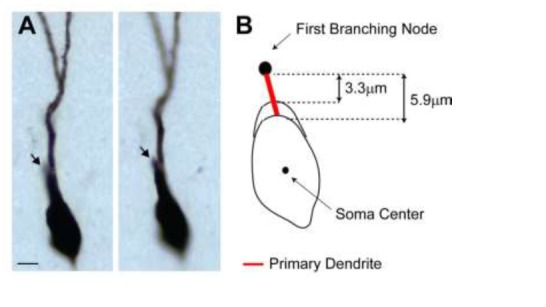
Morphometric analysis of the reconstructed neurons was performed with the Neurolucida software. Neuronal reconstructions were performed blind to the electrophysiological properties of the cells. For cell id 993, the soma was occluded by a black deposit on the brain section, and its position was manually interpolated at the termination point of the primary dendrite. Close-up magnifications of the soma and proximal dendrites in Figure 4—figure supplement 1 have, in a few cases, been rotated along the longitudinal axis to allow optimal display of the primary dendrites. The quality of cellular filling and labeling was estimated by quantifying the gray levels of DAB-stained neurons with ImageJ (Schneider et al., 2012). For all identified neurons (n=13; Figure 4—figure supplement 1), high-magnification pictures (100x oil-immersion objective) were obtained under identical settings (e.g. illumination and camera exposure) with a light microscope (BX-53, Olympus). A region of interest was defined on proximal and distal dendrites, and the normalized gray scale values (max gray value – background level) were taken as a correlate of labeling intensities. All proximal dendritic segments were within 20 µm of the soma, while distal dendritic segments were ≥ 200 µm from the soma. We note that in both groups (active and silent) of reconstructed neurons, it cannot be assured whether - even in the best-filled examples - dendritic morphologies are full and complete. Nevertheless, our analysis indicates that labeling quality and filling efficiency were very similar between active and silent neurons (Figure 4—figure supplement 2B–D and ‘control experiments’ below). Labeling efficiencies for silent and active neurons were estimated as the proportion of filled neurons (n=6 active and n=7 silent neurons; Figure 4—figure supplement 1 and Figure 4—source data 1) over all labeling attempts. Dendritic lengths were not compensated by tissue shrinkage. Dendritic order (nth) was defined as the portion of the dendritic tree between the (n−1) and (n) branching nodes, or the dendritic end. The only exception was the first-order dendrites, which were estimated as the distance between the soma center and the first branching node. We found this measure to be more consistent across repeated measurements and experimenters, whereas the distance from the soma edge to the first branching node is more dependent on the shape (more or less elongated) of the somatic contour. Estimating primary dendritic length as the distance between the soma edge and the first branching node (see dendritic segments in ‘blue’ in Figure 4—figure supplement 1) did not affect classification accuracy (not shown). The ‘soma location’ within the GC layer (see Figure 4—source data 1) was estimated as the relative position with respect to the anatomical borders of the GC layer, with ‘0’ representing the deep border – close to the hilus – and ‘1’ the superficial border – close to the molecular layer. The ‘branching index’ was defined as the number of dendritic endings divided by the number of primary dendrites. The ‘complexity index’ was computed, as in previous work (Pillai et al., 2012), according to the following equation: (Σ branch tip orders + number of branch tips)×(total dendritic length/total number of primary dendrites). To estimate the total number of spines (see Figure 4—source data 1), we quantified spine densities in GCs (n=7) by manually counting the number of spines on 10 µm dendritic segments, and then dividing it by the total segment length; at least three dendritic segments were counted per branch order, and averaged. Spine densities were within the range reported in the literature (Desmond and Levy, 1985; Hama et al., 1989; Trommald and Hulleberg, 1997; Vuksic et al., 2008; Freiman et al., 2011); however, in the present study, densities were not compensated for hidden spines and so absolute values represent an underestimate. Since spine densities increased as a function of dendritic order (not shown; see also Stone et al. (2011)), the total number of spines (Figure 4—source data 1) was estimated as the sum, over all dendritic orders, of the spine densities multiplied by the total dendritic length of each order.

Morphological analysis: control experiments

To determine whether the morphological differences between active and silent neurons could have resulted from procedural or methodological biases, we preformed the following controls. First, the efficiency of juxtacellular filling was very similar between active and silent neurons (active, 6/14 labeling attempts, ~42%; silent, 7/19 labeling attempts, ~37%). Second, no apparent bias was observed in the distribution of active and silent neurons across animals (Figure 4—figure supplement 2A), and no correlation was observed between in-vivo activity and soma location within the GC layer or the laminar location of the cells (suprapyramidal versus infrapyramidal blade) (see Figure 4—source data 1). Third, the quality of cell filling and dendritic labeling was similar between active and silent neurons. This was assessed by comparing: (i) the staining intensity at distal dendritic locations (Figure 4—figure supplement 2B,C); and (ii) the distribution of dendritic endings as a function of distance from the soma (Figure 4—figure supplement 2D). We reasoned that incompletely filled neurons should display lower labeling intensities and dendritic endings that are located closer to the soma; these parameters (together with total dendritic lengths, see Figure 4—source data 1) were not significantly different between active and silent neurons (see Figure 4—figure supplement 2B–D). Moreover, dendritic complexity was not correlated to the labeling/filling quality (p=0.32; n=13). Altogether,these analyses indicate that our identified neurons are likely to represent a random sample of active and silent GCs, and that labeling biases are unlikely to account for the differences in morphological parameters between the two classes.

Sparse logistic regression classifier

To build an automatic cell-type classifier that uses morphological parameters, we trained an L1-regularized logistic regression classifier (Friedman et al., 2010) using nested cross-validation (Cadwell et al., 2016). In the outer cross-validation loop, we iterated over each individual cell, evaluating the prediction for that cell with a model trained on all but that cell (‘leave-one-out cross-validation’). We used primary dendritic measures (the total dendritic length, the length of dendritic orders 1–7, the number of primary dendrites and the number of dendritic endings) as features (10 in total; see Figure 4D). Training on additional derived measures (such as ‘complexity index’ or ‘branching index’; see Figure 4—source data 1) did not improve classification performance (not shown; see Figure 4—source code 1).

Cross-validation in the inner loop was used to select the optimal amount of regularization. The evaluated model is selected on the basis of the the 1-SE rule to prevent overfitting (Friedman et al., 2010). All variables were z-scored before training the classifier. We used the elastic-net algorithm with α=0.05, 0.1, 0.5, 0.9 and 0.95, regularizing the weights with a mix of L2 and L1 regularization; this resulted in a denser weight vector for small values of α and a sparse weight vector for high values. The elastic-net penalty is particularly well suited for coping with highly correlated predictors as is the case here (Friedman et al., 2010). The choice of α did not affect the classification performance (~85%). We used the implementation provided by lassoglm in MATLAB with a binomial output distribution. We report the mean weight with SEM across cross-validation runs. To test whether the classification performance is significantly different than chance, we performed a permutation test. To this end, we shuffled the labels of all cells and repeated the entire cross-validation and classification procedure to obtain a null distribution of classification performances (500 runs, only for α=0.1). The p-value for the classification performance on the actual data is computed as the fraction of runs resulting in a classification performance larger or equal to the one observed in the data. Code for running this analysis is available with the paper (Figure 4—source code 1).

Acknowledgements

This work was supported by the Werner Reichardt Centre for Integrative Neuroscience (CIN) at the Eberhard Karls University of Tübingen (CIN is an Excellence Cluster funded by the Deutsche Forschungsgemeinschaft within the framework of the Excellence Initiative EXC 307) and by the the Bernstein Award from the German Ministry of Science and Education (BMBF) to PB (FKZ 01GQ1601). We thank Alexandra Eritja for excellent assistance with anatomy experiments, and Nima Ghorbani for contributing to software development. We thank James Knierim and Xioajing Chen for helpful discussions.

Funding Statement

The funders had no role in study design, data collection and interpretation, or the decision to submit the work for publication.

Funding Information

This paper was supported by the following grants:

  • Deutsche Forschungsgemeinschaft EXC 307 to Maria Diamantaki, Markus Frey, Philipp Berens, Patricia Preston-Ferrer, Andrea Burgalossi.

  • Bundesministerium für Bildung und Forschung FKZ 01GQ1601 to Philipp Berens.

Additional information

Competing interests

The authors declare that no competing interests exist.

Author contributions

MD, Acquisition of data, Analysis and interpretation of data, Drafting or revising the article.

MF, Analysis and interpretation of data, Drafting or revising the article.

PB, Analysis and interpretation of data, Drafting or revising the article.

PP-F, Conception and design, Acquisition of data, Analysis and interpretation of data, Drafting or revising the article.

AB, Conception and design, Acquisition of data, Analysis and interpretation of data, Drafting or revising the article.

Ethics

Animal experimentation: All experimental procedures were performed according to the German guidelines on animal welfare and approved by the local institution in charge of experiments using animals (Regierungspraesidium Tuebingen, permit numbers CIN2/14, CIN/5/14 and CIN/814).

References

  1. Alme CB, Buzzetti RA, Marrone DF, Leutgeb JK, Chawla MK, Schaner MJ, Bohanick JD, Khoboko T, Leutgeb S, Moser EI, Moser MB, McNaughton BL, Barnes CA. Hippocampal granule cells opt for early retirement. Hippocampus. 2010;20:1109–1123. doi: 10.1002/hipo.20810. [DOI] [PubMed] [Google Scholar]
  2. Amaral DG, Woodward DJ. A hippocampal interneuron observed in the inferior region. Brain Research. 1977;124:225–236. doi: 10.1016/0006-8993(77)90881-2. [DOI] [PubMed] [Google Scholar]
  3. Ambrogini P, Lattanzi D, Ciuffoli S, Agostini D, Bertini L, Stocchi V, Santi S, Cuppini R. Morpho-functional characterization of neuronal cells at different stages of maturation in granule cell layer of adult rat dentate gyrus. Brain Research. 2004;1017:21–31. doi: 10.1016/j.brainres.2004.05.039. [DOI] [PubMed] [Google Scholar]
  4. Barth AL, Poulet JF. Experimental evidence for sparse firing in the neocortex. Trends in Neurosciences. 2012;35:345–355. doi: 10.1016/j.tins.2012.03.008. [DOI] [PubMed] [Google Scholar]
  5. Bjerknes TL, Moser EI, Moser MB, Edvard MI. Representation of geometric borders in the developing rat. Neuron. 2014;82:71–78. doi: 10.1016/j.neuron.2014.02.014. [DOI] [PubMed] [Google Scholar]
  6. Brecht M, Schneider M, Sakmann B, Margrie TW. Whisker movements evoked by stimulation of single pyramidal cells in rat motor cortex. Nature. 2004;427:704–710. doi: 10.1038/nature02266. [DOI] [PubMed] [Google Scholar]
  7. Burgalossi A, Herfst L, von Heimendahl M, Förste H, Haskic K, Schmidt M, Brecht M. Microcircuits of functionally identified neurons in the rat medial entorhinal cortex. Neuron. 2011;70:773–786. doi: 10.1016/j.neuron.2011.04.003. [DOI] [PubMed] [Google Scholar]
  8. Burgalossi A, von Heimendahl M, Brecht M. Deep layer neurons in the rat medial entorhinal cortex fire sparsely irrespective of spatial novelty. Frontiers in Neural Circuits. 2014;8:e20252. doi: 10.3389/fncir.2014.00074. [DOI] [PMC free article] [PubMed] [Google Scholar]
  9. Buzsáki G, Mizuseki K. The log-dynamic brain: how skewed distributions affect network operations. Nature Reviews Neuroscience. 2014;15:264–278. doi: 10.1038/nrn3687. [DOI] [PMC free article] [PubMed] [Google Scholar]
  10. Cadwell CR, Palasantza A, Jiang X, Berens P, Deng Q, Yilmaz M, Reimer J, Shen S, Bethge M, Tolias KF, Sandberg R, Tolias AS. Electrophysiological, transcriptomic and morphologic profiling of single neurons using Patch-seq. Nature Biotechnology. 2016;34:199–203. doi: 10.1038/nbt.3445. [DOI] [PMC free article] [PubMed] [Google Scholar]
  11. Cameron HA, McKay RD. Adult neurogenesis produces a large pool of new granule cells in the dentate gyrus. The Journal of Comparative Neurology. 2001;435:406–417. doi: 10.1002/cne.1040. [DOI] [PubMed] [Google Scholar]
  12. Crochet S, Poulet JF, Kremer Y, Petersen CC, Poulet James FA. Synaptic mechanisms underlying sparse coding of active touch. Neuron. 2011;69:1160–1175. doi: 10.1016/j.neuron.2011.02.022. [DOI] [PubMed] [Google Scholar]
  13. Danielson NB, Kaifosh P, Zaremba JD, Lovett-Barron M, Tsai J, Denny CA, Balough EM, Goldberg AR, Drew LJ, Hen R, Losonczy A, Kheirbek MA. Distinct Contribution of Adult-Born Hippocampal Granule Cells to Context Encoding. Neuron. 2016;90:101–112. doi: 10.1016/j.neuron.2016.02.019. [DOI] [PMC free article] [PubMed] [Google Scholar]
  14. Desmond NL, Levy WB. Granule cell dendritic spine density in the rat hippocampus varies with spine shape and location. Neuroscience Letters. 1985;54:219–224. doi: 10.1016/s0304-3940(85)80082-3. [DOI] [PubMed] [Google Scholar]
  15. Diamantaki M, Frey M, Preston-Ferrer P, Burgalossi A. Priming spatial activity by single-cell stimulation in the dentate gyrus of freely moving rats. Current Biology . 2016;26:536–541. doi: 10.1016/j.cub.2015.12.053. [DOI] [PubMed] [Google Scholar]
  16. Doron G, von Heimendahl M, Schlattmann P, Houweling AR, Brecht M. Spiking irregularity and frequency modulate the behavioral report of single-neuron stimulation. Neuron. 2014;81:653–663. doi: 10.1016/j.neuron.2013.11.032. [DOI] [PubMed] [Google Scholar]
  17. Epsztein J, Brecht M, Lee AK. Intracellular determinants of hippocampal CA1 place and silent cell activity in a novel environment. Neuron. 2011;70:109–120. doi: 10.1016/j.neuron.2011.03.006. [DOI] [PMC free article] [PubMed] [Google Scholar]
  18. Espósito MS, Piatti VC, Laplagne DA, Morgenstern NA, Ferrari CC, Pitossi FJ, Schinder AF. Neuronal differentiation in the adult hippocampus recapitulates embryonic development. Journal of Neuroscience. 2005;25:10074–10086. doi: 10.1523/JNEUROSCI.3114-05.2005. [DOI] [PMC free article] [PubMed] [Google Scholar]
  19. Freiman TM, Eismann-Schweimler J, Frotscher M. Granule cell dispersion in temporal lobe epilepsy is associated with changes in dendritic orientation and spine distribution. Experimental Neurology. 2011;229:332–338. doi: 10.1016/j.expneurol.2011.02.017. [DOI] [PubMed] [Google Scholar]
  20. Friedman J, Hastie T, Tibshirani R. Regularization paths for generalized linear models via coordinate descent. Journal of Statistical Software. 2010;33:1–22. doi: 10.18637/jss.v033.i01. [DOI] [PMC free article] [PubMed] [Google Scholar]
  21. Gould E. Structural plasticity. In: Andersen P, Morris R, Amaral D, Bliss T, O'Keefe J, editors. The Hippocampus Book. Oxford University Press; 2006. [Google Scholar]
  22. Haibo H, Yang B, Garcia EA, Shutao L. ADASYN: Adaptive synthetic sampling approach for imbalanced learning. Neural Networks (IEEE World Congress on Computational Intelligence) IEEE International Joint Conference; 2008. pp. 1322–1328. [Google Scholar]
  23. Hama K, Arii T, Kosaka T. Three-dimensional morphometrical study of dendritic spines of the granule cell in the rat dentate gyrus with HVEM stereo images. Journal of Electron Microscopy Technique. 1989;12:80–87. doi: 10.1002/jemt.1060120203. [DOI] [PubMed] [Google Scholar]
  24. Herfst L, Burgalossi A, Haskic K, Tukker JJ, Schmidt M, Brecht M. Friction-based stabilization of juxtacellular recordings in freely moving rats. Journal of Neurophysiology. 2012;108:697–707. doi: 10.1152/jn.00910.2011. [DOI] [PMC free article] [PubMed] [Google Scholar]
  25. Houweling AR, Brecht M. Behavioural report of single neuron stimulation in somatosensory cortex. Nature. 2008;451:65–68. doi: 10.1038/nature06447. [DOI] [PubMed] [Google Scholar]
  26. Hromádka T, Deweese MR, Zador AM. Sparse representation of sounds in the unanesthetized auditory cortex. PLoS Biology. 2008;6:e20252. doi: 10.1371/journal.pbio.0060016. [DOI] [PMC free article] [PubMed] [Google Scholar]
  27. Huber D, Petreanu L, Ghitani N, Ranade S, Hromádka T, Mainen Z, Svoboda K. Sparse optical microstimulation in barrel cortex drives learned behaviour in freely moving mice. Nature. 2008;451:61–64. doi: 10.1038/nature06445. [DOI] [PMC free article] [PubMed] [Google Scholar]
  28. Jung MW, McNaughton BL. Spatial selectivity of unit activity in the hippocampal granular layer. Hippocampus. 1993;3:165–182. doi: 10.1002/hipo.450030209. [DOI] [PubMed] [Google Scholar]
  29. Klausberger T, Magill PJ, Márton LF, Roberts JD, Cobden PM, Buzsáki G, Somogyi P. Brain-state- and cell-type-specific firing of hippocampal interneurons in vivo. Nature. 2003;421:844–848. doi: 10.1038/nature01374. [DOI] [PubMed] [Google Scholar]
  30. Leutgeb JK, Leutgeb S, Moser MB, Moser EI. Pattern separation in the dentate gyrus and CA3 of the hippocampus. Science. 2007;315:961–966. doi: 10.1126/science.1135801. [DOI] [PubMed] [Google Scholar]
  31. Li CY, Poo MM, Dan Y. Burst spiking of a single cortical neuron modifies global brain state. Science. 2009;324:643–646. doi: 10.1126/science.1169957. [DOI] [PMC free article] [PubMed] [Google Scholar]
  32. Lisman J. Formation of the non-functional and functional pools of granule cells in the dentate gyrus: role of neurogenesis, LTP and LTD. The Journal of Physiology. 2011;589:1905–1909. doi: 10.1113/jphysiol.2010.201137. [DOI] [PMC free article] [PubMed] [Google Scholar]
  33. Martí-Subirana A, Soriano E, García-Verdugo JM. Morphological aspects of the ectopic granule-like cellular populations in the albino rat hippocampal formation: a Golgi study. Journal of Anatomy. 1986;144:31–47. [PMC free article] [PubMed] [Google Scholar]
  34. McNaughton B, Morris R. Hippocampal synaptic enhancement and information storage within a distributed memory system. TINS. 1987;10:408–415. doi: 10.1016/0166-2236(87)90011-7. [DOI] [Google Scholar]
  35. Mizuseki K, Buzsáki G. Preconfigured, skewed distribution of firing rates in the hippocampus and entorhinal cortex. Cell Reports. 2013;4:1010–1021. doi: 10.1016/j.celrep.2013.07.039. [DOI] [PMC free article] [PubMed] [Google Scholar]
  36. Myers CE, Scharfman HE. A role for hilar cells in pattern separation in the dentate gyrus: a computational approach. Hippocampus. 2009;19:321–337. doi: 10.1002/hipo.20516. [DOI] [PMC free article] [PubMed] [Google Scholar]
  37. Neunuebel JP, Knierim JJ. Spatial firing correlates of physiologically distinct cell types of the rat dentate gyrus.  Journal of Neuroscience. 2012;32:3848–3858. doi: 10.1523/JNEUROSCI.6038-11.2012. [DOI] [PMC free article] [PubMed] [Google Scholar]
  38. Neunuebel JP, Knierim JJ. CA3 retrieves coherent representations from degraded input: direct evidence for CA3 pattern completion and dentate gyrus pattern separation. Neuron. 2014;81:416–427. doi: 10.1016/j.neuron.2013.11.017. [DOI] [PMC free article] [PubMed] [Google Scholar]
  39. O'Connor DH, Peron SP, Huber D, Svoboda K. Neural activity in barrel cortex underlying vibrissa-based object localization in mice. Neuron. 2010;67:1048–1061. doi: 10.1016/j.neuron.2010.08.026. [DOI] [PubMed] [Google Scholar]
  40. Olshausen BA, Field DJ. Sparse coding of sensory inputs. Current Opinion in Neurobiology. 2004;14:481–487. doi: 10.1016/j.conb.2004.07.007. [DOI] [PubMed] [Google Scholar]
  41. Pernía-Andrade AJ, Jonas P. Theta-gamma-modulated synaptic currents in hippocampal granule cells in vivo define a mechanism for network oscillations. Neuron. 2014;81:140–152. doi: 10.1016/j.neuron.2013.09.046. [DOI] [PMC free article] [PubMed] [Google Scholar]
  42. Pillai AG, de Jong D, Kanatsou S, Krugers H, Knapman A, Heinzmann JM, Holsboer F, Landgraf R, Joëls M, Touma C. Dendritic morphology of hippocampal and amygdalar neurons in adolescent mice is resilient to genetic differences in stress reactivity. PLoS One. 2012;7:e20252. doi: 10.1371/journal.pone.0038971. [DOI] [PMC free article] [PubMed] [Google Scholar]
  43. Pinault D. A novel single-cell staining procedure performed in vivo under electrophysiological control: morpho-functional features of juxtacellularly labeled thalamic cells and other central neurons with biocytin or Neurobiotin. Journal of Neuroscience Methods. 1996;65:113–136. doi: 10.1016/0165-0270(95)00144-1. [DOI] [PubMed] [Google Scholar]
  44. Ray S, Naumann R, Burgalossi A, Tang Q, Schmidt H, Brecht M. Grid-layout and theta-modulation of layer 2 pyramidal neurons in medial entorhinal cortex. Science. 2014;343:891–896. doi: 10.1126/science.1243028. [DOI] [PubMed] [Google Scholar]
  45. Rochefort NL, Garaschuk O, Milos R-I, Narushima M, Marandi N, Pichler B, Kovalchuk Y, Konnerth A. Sparsification of neuronal activity in the visual cortex at eye-opening. PNAS. 2009;106:15049–15054. doi: 10.1073/pnas.0907660106. [DOI] [PMC free article] [PubMed] [Google Scholar]
  46. Scharfman H, Goodman J, McCloskey D. Ectopic granule cells of the rat dentate gyrus. Developmental Neuroscience. 2007;29:14–27. doi: 10.1159/000096208. [DOI] [PMC free article] [PubMed] [Google Scholar]
  47. Scharfman HE, Pierce JP. New insights into the role of hilar ectopic granule cells in the dentate gyrus based on quantitative anatomic analysis and three-dimensional reconstruction. Epilepsia. 2012;53:109–115. doi: 10.1111/j.1528-1167.2012.03480.x. [DOI] [PMC free article] [PubMed] [Google Scholar]
  48. Schmidt-Hieber C, Jonas P, Bischofberger J. Enhanced synaptic plasticity in newly generated granule cells of the adult hippocampus. Nature. 2004;429:184–187. doi: 10.1038/nature02553. [DOI] [PubMed] [Google Scholar]
  49. Schneider CA, Rasband WS, Eliceiri KW. NIH Image to ImageJ: 25 years of image analysis. Nature Methods. 2012;9:671–675. doi: 10.1038/nmeth.2089. [DOI] [PMC free article] [PubMed] [Google Scholar]
  50. Skaggs WE, McNaughton BL, Wilson MA, Barnes CA. Theta phase precession in hippocampal neuronal populations and the compression of temporal sequences. Hippocampus. 1996;6:149–172. doi: 10.1002/(SICI)1098-1063(1996)6:2&#x0003c;149::AID-HIPO6&#x0003e;3.0.CO;2-K. [DOI] [PubMed] [Google Scholar]
  51. Spanne A, Jörntell H. Questioning the role of sparse coding in the brain. Trends in Neurosciences. 2015;38:417–427. doi: 10.1016/j.tins.2015.05.005. [DOI] [PubMed] [Google Scholar]
  52. Stone SS, Teixeira CM, Devito LM, Zaslavsky K, Josselyn SA, Lozano AM, Frankland PW. Stimulation of entorhinal cortex promotes adult neurogenesis and facilitates spatial memory. Journal of Neuroscience. 2011;31:13469–13484. doi: 10.1523/JNEUROSCI.3100-11.2011. [DOI] [PMC free article] [PubMed] [Google Scholar]
  53. Szabadics J, Varga C, Brunner J, Chen K, Soltesz I. Granule cells in the CA3 area. Journal of Neuroscience. 2010;30:8296–8307. doi: 10.1523/JNEUROSCI.5602-09.2010. [DOI] [PMC free article] [PubMed] [Google Scholar]
  54. Tang Q, Brecht M, Burgalossi A. Juxtacellular recording and morphological identification of single neurons in freely moving rats. Nature Protocols. 2014a;9:2369–2381. doi: 10.1038/nprot.2014.161. [DOI] [PubMed] [Google Scholar]
  55. Tang Q, Burgalossi A, Ebbesen CL, Ray S, Naumann R, Schmidt H, Spicher D, Brecht M. Pyramidal and stellate cell specificity of grid and border representations in layer 2 of medial entorhinal cortex. Neuron. 2014b;84:1191–1197. doi: 10.1016/j.neuron.2014.11.009. [DOI] [PMC free article] [PubMed] [Google Scholar]
  56. Tang Q, Burgalossi A, Ebbesen CL, Sanguinetti-Scheck JI, Schmidt H, Tukker JJ, Naumann R, Ray S, Preston-Ferrer P, Schmitz D, Brecht M. Functional architecture of the rat parasubiculum. Journal of Neuroscience. 2016;36:2289–2301. doi: 10.1523/JNEUROSCI.3749-15.2016. [DOI] [PMC free article] [PubMed] [Google Scholar]
  57. Tang Q, Ebbesen CL, Sanguinetti-Scheck JI, Preston-Ferrer P, Gundlfinger A, Winterer J, Beed P, Ray S, Naumann R, Schmitz D, Brecht M, Burgalossi A. Anatomical organization and spatiotemporal firing patterns of layer 3 neurons in the rat medial entorhinal cortex. Journal of Neuroscience. 2015;35:12346–12354. doi: 10.1523/JNEUROSCI.0696-15.2015. [DOI] [PMC free article] [PubMed] [Google Scholar]
  58. Treves A, Rolls ET. Computational analysis of the role of the hippocampus in memory. Hippocampus. 1994;4:374–391. doi: 10.1002/hipo.450040319. [DOI] [PubMed] [Google Scholar]
  59. Trommald M, Hulleberg G. Dimensions and density of dendritic spines from rat dentate granule cells based on reconstructions from serial electron micrographs. The Journal of Comparative Neurology. 1997;377:15–28. doi: 10.1002/(SICI)1096-9861(19970106)377:1&#x0003c;15::AID-CNE3&#x0003e;3.0.CO;2-M. [DOI] [PubMed] [Google Scholar]
  60. Tóth K, Freund TF. Calbindin D28k-containing nonpyramidal cells in the rat hippocampus: their immunoreactivity for GABA and projection to the medial septum. Neuroscience. 1992;49:793–805. doi: 10.1016/0306-4522(92)90357-8. [DOI] [PubMed] [Google Scholar]
  61. Vuksic M, Del Turco D, Bas Orth C, Burbach GJ, Feng G, Müller CM, Schwarzacher SW, Deller T. 3D-reconstruction and functional properties of GFP-positive and GFP-negative granule cells in the fascia dentata of the Thy1-GFP mouse. Hippocampus. 2008;18:364–375. doi: 10.1002/hipo.20398. [DOI] [PubMed] [Google Scholar]
  62. Wolfe J, Houweling AR, Brecht M. Sparse and powerful cortical spikes. Current Opinion in Neurobiology. 2010;20:306–312. doi: 10.1016/j.conb.2010.03.006. [DOI] [PubMed] [Google Scholar]
  63. Zhao C, Teng EM, Summers RG, Ming GL, Gage FH. Distinct morphological stages of dentate granule neuron maturation in the adult mouse hippocampus. Journal of Neuroscience. 2006;26:3–11. doi: 10.1523/JNEUROSCI.3648-05.2006. [DOI] [PMC free article] [PubMed] [Google Scholar]
eLife. 2016 Oct 3;5:e20252. doi: 10.7554/eLife.20252.014

Decision letter

Editor: Karel Svoboda1

In the interests of transparency, eLife includes the editorial decision letter and accompanying author responses. A lightly edited version of the letter sent to the authors after peer review is shown, indicating the most substantive concerns; minor comments are not usually included.

Thank you for submitting your article "Structural determinants of granule cell activity in the dentate gyrus of freely-moving rats" for consideration by eLife. Your article has been favorably evaluated by Eve Marder (Senior Editor) and three reviewers, one of whom, Karel Svoboda (Reviewer #1), is a member of our Board of Reviewing Editors, and another one is Matthew F Nolan (Reviewer #2).

The reviewers have discussed the reviews with one another and the Reviewing Editor has drafted this decision to help you prepare a revised submission.

Summary:

This manuscript describes loose-seal cell-attached recordings from hippocampal granule cells (GCs) in awake rats. We know relatively little about these mysterious cells. Previous experiments have explored granule cell activity using tetrode-style recordings or maps of cFos expression. These methods have suggested that GC activity is sparse – in the sense that only a small subset of GCs are active in any one environment – but both methods are imperfect. Extracellular recordings are biased towards active cells and sample neurons with more membrane area more efficiently. Loose-seal recordings are unbiased in the sense that active and inactive neurons are recorded. The authors find ultra-sparse activity in GCs, providing the strongest evidence to data for sparse coding in the dentate gyrus. Loose-seal recordings in addition allow labeling and reconstruction of a subset of recorded neurons. This provides the additional insight that active neurons are larger and spiny. This is a nice and simple structure-function relationship. These findings of specific structure-function relationships within the (mature) dentate granule cell population are novel and very interesting, and would constitute a valuable contribution to the field.

Essential revisions:

All reviewers have reservations about the strength of the statistical analysis used to support the main conclusions and presentation of the data. We suggest that you take the comments below as a guide to reanalyze the data set.

1) Details on the GC recordings and morphological parameters should be provided. We suggest a supplementary table containing all neurons as separate entries with these data: duration of recording; number of spikes recorded; identity of the animal; duration of the recording; distance covered by the animal; aspects of receptive field shape (i.e. place field attributes), morphological parameters; which analysis and figure the neuron contributed to. This table should allow independent analysis of the dataset. The detailed dendritic structures should be deposited at neuromorph.org or another repository.

2) Given multiple comparisons of dendritic structure were made, it is unclear if corrections for multiple comparisons were made. This is related to the hot topic of 'p-value hacking'. Please make sure to take multiple comparisons into account.

3) The study reports numbers of neurons, treating each neuron as an independent observation. Could the apparent relationship between activity and dendrite morphology instead reflect a subset of animals in which granule cells are more active with more complex dendrites? The possibility of non-independence of observations should be accounted for in the statistical analysis.

4) The description of the classifier and its evaluation is not sufficient. What properties of the spike waveform were used for training? What was the exact composition of the training and test datasets? Is it just the 47 neurons in Figure 1D? This is a somewhat small number of samples compared to datasets often used for training classifiers. What was the false positive and false negative rate when testing the classifier? What was the quantitative criterion for shoulder or no shoulder in Figure 1D? Figure 1G indicates that the shoulder is variable and not present in all granule cells. Does this have implications for interpretation of the data and what are these?

5) Figure 4D. The legend indicates that "the distributions" are statistically different. Is this referring to length, distance, or length data as a function of distance as shown in the figure? The conclusion is based on results of a Mann Whitney U which would usually be used to test for a difference in medians. It is not clear how this was applied here.

The analysis of morphology and its presentation needs to be improved. Assuming that the morphologies of the 7 silent and 6 active granule cells analyzed in detail are complete and representative, the main conclusions of the study are fairly straightforward. Therefore, it is important for the authors to devote more of the manuscript to their morphological methods and clarify their procedures in more detail.

6) The authors write "we reconstructed the somato-dendritic compartment of 7 silent and 6 active GCs, which were selected for the morphological analysis due to their high-quality filling and complete dendritic morphology." What were the criteria for assessing the completeness of the dendritic morphology? Was the labeling protocol standardized in some way between silent and active neurons? For instance, is it possible that it was harder to fill silent cells than active ones? What is the fraction of silent cells for which labeling was attempted whose dendritic tree was completely filled, and how does that compare to the fraction for active cells? If there was any difference in the rate of complete filling, could it be possible that there was a bias in the labeling method that could lead to an apparent difference in the level of branching or complexity? Is it possible, for example, that silent cells were harder to fill and more likely to have somewhat less complete dendritic fills, and thus more likely to appear to have less complex trees?

7) The branching and complexity measures that show a difference between active and silent cells are defined in the methods: "The 'branching index' was defined as the number of dendritic endings divided by the number of primary dendrites. The 'complexity index' was computed as in previous work (Pillai et al., 2012) according to the following equation: (sum of branch tip orders + number of branch tips) x (total dendritic length/total number of primary dendrites)." These measures appear to be particularly sensitive to the number of primary dendrites as it appears in the denominator in both cases. Therefore, the authors should include in the table mentioned above, for each of the 13 neurons with complete dendritic trees, the firing rate in the arena, the branching and complexity values, the total dendritic length, the number of dendritic endings, and the number of primary dendrites. The authors write that there was a non-significant 2x difference in the number of primary dendrites "(the number of primary dendrites (active, 1.1+/-0.4; silent, 2.2+/-1.1; p=0.08)", but the branching index also differed by 2x "(branching index; active, 14.6+/-4.6; silent, 7.8+/-4.7; p=0.026)", though this difference was significant. This suggests that the number of dendritic endings is similar for both silent and active cells. Therefore, is it possible that the difference in the number of primary dendrites could be responsible for differences in activity, instead of the difference in spine number that they suggest as the cause? In comparison, the number of spines differed by a factor of 1.4x "(total number of spines; active, 1802+/-353; silent, 1354+/-257; p=0.035)" and they state "The total number of dendritic spines also showed a significant correlation with firing rates (r=0.63; p=0.019; n=13)". What is the correlation between the number of primary dendrites and firing rate and associated significance?

8) The authors write that "The large majority of sampled neurons were silent (see Figure 2F). In order to record from spiking GCs, silent recordings were routinely discarded by further advancing the electrode within the layer." Does this mean that their sample was biased toward more active cells? If so, they should clearly point this out when they state proportions of cells that were active. For instance, they state "Active GCs were thus very sparse, consistent with previous estimates (Jung and McNaughton, 1993; Leutgeb et al., 2007; Neunuebel and Knierim, 2012) and accounted for only ~14% (32 out of 228) of all blindly-sampled neurons within the GC layer." If they biased their search for active cells, then they should remove "blindly-sampled" from this sentence and point out that the 14% value is an overestimate based on their sampling method. In addition, is it possible that any bias in the search toward active cells could influence the morphological results? For instance, is it possible that cells that are active during the search and active during exploration of the arena are not a random sample of the entire set of cells active during exploration? Perhaps these cells have more branching and complex dendritic trees compared to cells that are active during exploration but were not spontaneously active during the cell search procedure? The basic question is whether the sample of 7 silent and 6 active cells analyzed in detail morphologically constituted an unbiased sample of silent cells, and an unbiased sample of active cells, respectively. If the possibility of such a bias cannot be ruled out, yet there is no reason to think there is a bias, the authors could just make a short comment about how they assume their methods have isolated a random sample of silent and active cells.

How long did they wait before discarding silent cells? This defines an upper bound on the possible spike rate of silent cells.

The authors recently showed that they could induce place fields in some granule cells by juxtacellular electrical stimulation (Diamantaki et al. 2016). Does this effect also correlate with dendritic structure? Please discuss.

The paper should be more tightly framed in terms of measurement of sparseness (additional literature should be cited) and structure-function-relationship.

[Editors’ note: a previous version of this study was rejected after a second round of peer review, but the authors submitted for reconsideration. The decision letter after this second round of review is shown below.]

Thank you for submitting your work entitled "Structural correlates of granule cell activity in the dentate gyrus of freely-moving rats" for consideration by eLife. Your article has been reviewed by two peer reviewers, and the evaluation has been overseen by a Reviewing Editor (Karel Svoboda) and Eve Marder as the Senior Editor. The following individuals involved in review of your submission have agreed to reveal their identity: Karel Svoboda (Reviewer #1) and Matthew F Nolan (Reviewer #2).

Our decision has been reached after consultation between the Reviewing Editor and the reviewers. Based on these discussions and the individual reviews below, we regret to inform you that your work will not be considered further for publication in eLife.

We note that the reviewers remain very positive about the data set and the finding of sparse coding in the dentate gyrus. However, the focus of the manuscript is the link between activity and dendritic structure (the title is 'Structural correlates of granule cell activity in the dentate gyrus of freely-moving rats'). Given this focus all reviewers and the Reviewing Editor remain concerned about the statistical analysis linking activity and dendritic structure. Some commonly used measures of dendritic complexity, such as dendritic length and the number of primary dendrites, showed no significant effect, whereas some less intuitive measures (i.e. 'dendritic complexity') did, but at modest levels of significance. Most of the reported measures are related and thus not independent. There are some indications that the study may be underpowered to make conclusions about dendritic structure. We are not convinced that the results were corrected for multiple comparisons together in an appropriate manner. For these reasons we cannot publish your manuscript in its present form.

However, we would be happy to consider the manuscript again with one of the following major revisions:

1) A more compelling statistical analysis. This could take the form of a rigorous analysis of multiple comparisons. Alternatively, a reanalysis with randomly chosen 50% of the data might also be appropriate.

2) Addition of data that make the conclusions about structure-function relationships stronger.

3) A refocusing on sparse coding in the dentate gyrus.

Reviewer # 1:

The paper is improved in many ways. However, the analysis of dendritic complexity remains suggestive, but not convincing.

Was the study design a priori to test the relationship of spike rate and the specific measure of dendritic complexity? If so, the analysis is appropriate. However, if this was exploratory then the stats are weak. The reasons are as follows.

There is one effect – higher dendritic complexity for higher spike rates. All the positive effects come from the same data and follow from each other; thus there is no independent second measurement. Of course, If one does enough comparisons there is bound to be one that is 'significant' by chance. I don't see a proper analysis of multiple comparisons (this may be hard to do).

Multiple testing and reporting significant results produces a publication bias. In other words, statistically significant findings are reported, increasing the rate of false positives in the literature. This is a prime cause of the poor replication record in psychology, MRI, cancer, and likely systems neuroscience.

Figure 4F seems to have 11 points, not 13. It is hard to believe that the p value is < 0.01

Reviewer #2:

The manuscript is substantially improved. However, I'm not convinced the issues related to multiple comparisons have been adequately addressed (points 2 and 5 in the original review).

The investigation of the relationship between activity and morphology requires comparing many parameters. Of course, by chance some of these comparisons will turn out significant at a p < 0.05 level. At the moment this possibility is not accounted for in the interpretation of the data. The challenge here seems to be to introduce an appropriate correction.

Using the Benjamini & Hochberg method to correct the p-values most of the significant differences appear to go away. An exception appears to be the 'Dendritic Length Order' measure. Even here one should perhaps be a little cautious as additional comparisons were made and correcting for them would reduce the significance level further – it is unclear how many comparisons one should correct for.

Given these potential issues, the question is what to do. I appreciate the challenges in obtaining the data, but in a sense this makes it even more important to be rigorous in interpretation. One option might be to carry out additional experiments to try to replicate the results with the analysis focussed on specific planned comparisons. An alternative could be to clearly label the study as exploratory.

Different multiple comparison issues apply to Figure 4D. I also don't understand how total dendritic length can be similar between the two groups, but the area of the plots in 4D looks quite different.

Additional comments:

The table only includes a subset of the measurements used for the analysis. It would be more helpful if all measurements are included.

It's not clear why the Abstract reports correlations rather than results of comparisons between active and silent neurons.

The recording duration is longer for active than silent cells. Is this an issue?

Reviewer #3:

The authors have adequately addressed my questions and concerns. I have a few remaining comments:

From the table, the numbers that stand out most are the differences in the number of primary dendrites, even though this did not reach significance.

In the Abstract, the authors write "We found that the majority of neurons (163 of 190) were silent during exploration." However, I recommend that the authors remove the numbers since it reads as if it is an unbiased estimate of the fraction of silent neurons, but they confirmed in the response that this is likely to be underestimate due to their search procedure. Instead they could add "vast" in front of "majority" to make their point.

In the Figure 2 legend the authors write "Unlike extracellular recordings, juxtacellular sampling is not biased towards active cells, since silent neurons can also be recorded and their presence confirmed by current injection." This is followed by "Cumulative plot showing the firing rate distribution within the GC layer. Each red circle represents one neuron, sampled juxtacellularly within the GC layer (see Methods for details). Note the large proportion of silent neurons (163 out of 190) compared to active cells." However, as acknowledged by the authors, their sampling of the proportion of active and silent cells is likely to be biased due to their search procedure, where inactive cells were often discarded early during exploration, before the 60-second threshold they used for counting the cells. Because of this, I think this statement and the numbers could confuse the readers into thinking that these numbers are an unbiased estimate, and one that is a better estimate than obtained with other methods. It would be a better estimate if their cell search / counting procedure was unbiased, but apparently it was not. The correct proportion is an important number. The authors should therefore clarify this in the legend as they have done in the main text. For example, they could write in the legend "Note the large proportion of silent neurons (163 out of 190) compared to active cells. Furthermore, this proportion is likely to be an underestimate of the true silent proportion due to the details of the search procedure (see text and methods)."

[Editors’ note: what now follows is the decision letter after the authors submitted for reconsideration.]

Thank you for submitting your article "Sparse activity of identified dentate-gyrus granule cells during spatial exploration" for consideration by eLife. Your article has been favorably evaluated by Eve Marder (Senior Editor) and three reviewers, one of whom, Karel Svoboda (Reviewer #1), is a member of our Board of Reviewing Editors, and another one is Matthew F Nolan (Reviewer #2).

The reviewers have discussed the reviews with one another and the Reviewing Editor has drafted this decision to help you prepare a revised submission.

Summary:

This manuscript describes loose-seal cell-attached recordings from hippocampal granule cells (GCs) in awake rats. We know relatively little about these mysterious cells. Previous experiments have explored granule cell activity using tetrode-style recordings or maps of cFos expression. These methods have suggested that GC activity is sparse – in the sense that only a small subset of GCs are active in any one environment – but both methods are imperfect.

Extracellular recordings are biased towards active cells and sample neurons with more membrane area more efficiently. Loose-seal recordings are unbiased in the sense that active and inactive neurons are recorded. The authors find ultra-sparse activity in GCs, settling and quantifying the issue of sparseness in a definitive manner. Loose-seal recordings in addition allow labeling and reconstruction of a subset of recorded neurons.

This is a revised submission, which is more tightly focused on sparse coding in the dentate gyrus. The analysis of structure-function relationships is now done using a classifier with multiple structural parameters considered jointly. The classifier reveals that structure predicts function.

Essential revisions:

Although the classifier can use structure to predict function, the relationship is subtle and can't clearly be boiled down to simple measures (at least given the limited data set) (see also Figure 4—figure supplement 1). It would be good to make this last point clearer (the relevant statement in the Discussion is not accurate and should be revised).

Describe more clearly what a primary, as in 1st order, dendrite compared to a 2nd order dendrite. This is because (1) it appears from the table that this this would have a large effect on distinguishing active and silent cells, not just in terms of the total 1st order length, but also in terms of the total higher order lengths (since a 5th order branch would be a 4th order branch if the 2nd order branch it came from was instead called a 1st order branch), and (2) the table shows that the 1st order branches are generally short. Therefore, in the Figure 4—figure supplement 1 the authors should include beside each neuron a close-up of the somatic region showing the soma, 1st order branch(es), and start of 2nd order branches, ideally with markers to show where the divisions are.

It would be valuable to the community for the authors to include some of the data from the original manuscript in the source file on morphological parameters, such as the "soma location within the GC layer" and the "laminar location of the cells (suprapyramidal versus infrapyramidal blade)."

eLife. 2016 Oct 3;5:e20252. doi: 10.7554/eLife.20252.015

Author response


[…] Essential revisions:

All reviewers have reservations about the strength of the statistical analysis used to support the main conclusions and presentation of the data. We suggest that you take the comments below as a guide to reanalyze the data set.

1) Details on the GC recordings and morphological parameters should be provided. We suggest a supplementary table containing all neurons as separate entries with these data: duration of recording; number of spikes recorded; identity of the animal; duration of the recording; distance covered by the animal; aspects of receptive field shape (i.e. place field attributes), morphological parameters; which analysis and figure the neuron contributed to. This table should allow independent analysis of the dataset. The detailed dendritic structures should be deposited at neuromorph.org or another repository.

Along with the reviewers’ suggestion, we provide a more comprehensive overview of our dataset by including a table and 2 figure supplements. We have also contacted Giorgio Ascoli for depositing our reconstructed neurons at neuromorph.org, which will be readily uploaded upon acceptance.

We provide a table which includes the major electrophysiological and morphological properties of our reconstructed silent and active neurons (Figure 4 —source data 1). We have also included 2 additional figures, where we show the morphology of all reconstructed neurons (Figure 4—figure supplement 1) and spatial firing activity in our dataset (Figure 3—figure supplement 1). Cell ids are indicated in the corresponding figures and figure legends. These data are referred to in the revised Results (fourth and fifth paragraphs).

2) Given multiple comparisons of dendritic structure were made, it is unclear if corrections for multiple comparisons were made. This is related to the hot topic of 'p-value hacking'. Please make sure to take multiple comparisons into account.

Multiple comparisons were taken into account by performing a multivariate ANOVA with two independent groups (silent/active) for comparing dendritic morphological parameters (see Figure 4—source data 1). Post-hoc pairwise comparisons were assessed with a two-sided Mann-Whitney nonparametric test (95% confidence intervals).

This is specified in the revised Methods (end of last paragraph).

3) The study reports numbers of neurons, treating each neuron as an independent observation. Could the apparent relationship between activity and dendrite morphology instead reflect a subset of animals in which granule cells are more active with more complex dendrites? The possibility of non-independence of observations should be accounted for in the statistical analysis.

To address the reviewers’ comment, we now provide the distribution of our recordings across all rats (Figure 4—figure supplement 2A). As it can be seen in the histogram, each rat contributed on average a very low number of recordings (average recordings per rat, 3.2 ± 2.7; median = 2). This was primarily due to the fact that, in order to achieve unequivocal cell identification (which is crucial for resolving structure-function relationships) only very few electrode penetrations and labeling attempts (typically one) were performed per animal. In the subset of rats where a larger number of neurons was recorded (see Figure 4—figure supplement 2A), labeling was either not attempted, or cell identification could not be determined with certainty. As a consequence of this sparse sampling, the large majority of identified recordings (16 out of 17; 94%) can be considered as ‘independent’ observations, as they come from different rats. We also sought to test whether active neurons were ‘clustered’ in some rats. To this end, we focused on the subset of animals with ≥ 5 recordings (n=15 rats); we find that the occurrence of active neurons was not significantly different from their expected proportion from the population data (~14%; see corresponding p values from binomial test in Author response image 1).

Author response image 1. Distribution of recordings across animals.

Author response image 1.

Histogram showing the distribution of active (red) and silent recordings (blue) across animals. In the animals with a relatively larger number of recordings (≥5, n=15 rats), the occurrence of active neurons was not significantly different from their expected proportion from the population data (~14%). Corresponding p values from binomial test are shown.

DOI: http://dx.doi.org/10.7554/eLife.20252.012

Altogether this indicates that – considering also that animal age, housing and behavioral training were standardized across animals – the relationship between morphology and activity is unlikely to reflect a bias in a subset of animals. However, we acknowledge that, given the relatively small number of observations per rat, a dependency between rat identity and morphological properties cannot be rigorously tested and thus formally ruled out. We specify this in the revised manuscript (see below).

To address this point, we have included a new Figure 4—figure supplement 2. We refer to this analysis in the revised manuscript (Results, eighth paragraph and Methods, subsection “Targeting of the dentate gyrus and dataset of juxtacellular recordings”, second paragraph). We specify that a relationship between morphology and rat identity cannot be formally ruled out in our dataset (Figure legend of Figure 4—figure supplement 2A).

4) The description of the classifier and its evaluation is not sufficient. What properties of the spike waveform were used for training? What was the exact composition of the training and test datasets? Is it just the 47 neurons in Figure 1D? This is a somewhat small number of samples compared to datasets often used for training classifiers. What was the false positive and false negative rate when testing the classifier? What was the quantitative criterion for shoulder or no shoulder in Figure 1D? Figure 1G indicates that the shoulder is variable and not present in all granule cells. Does this have implications for interpretation of the data and what are these?

We apologize for not having provided sufficient information about the classifier. We now clarify that (i) the classifier was trained on average spike waveforms, that (ii) the classifier was trained on our dataset of identified neurons (n=47; as in Figure 1D), with a leave-one-out cross-validation, and (iii) we provide the false-positive and false-negative rates (false-positive: 2/47 = ~4%; false-negative: 3/47 = ~6%). We also acknowledge in the revised manuscript that, in line with the reviewers’ comment, our classification results rest on a relatively small training dataset. This is specified in the revised Results.

We would also like to clarify the rationale behind the use of the classifier in our study. Classification of neurons as ‘putative GCs’ is not strictly dependent upon the neural-network classifier approach; recordings are classified as ‘putative’ GCs by the occurrence of spike- shoulders, which were detected by the intersection between the spike trace and its moving average during the repolarization phase of the spike (more details are provided in the new Figure 1—figure supplement 1A). The neural-network classifier was implemented for testing whether recordings can also be assigned to the GC class based solely on their average spike waveforms. We believe that in this respect, the classification results provide additional evidence for a relationship between spike-shape and GC identity. This is now specified in the revised Results.

In line with the reviewers’ comments (i.e. ‘What properties of the spike waveform were used for training?’),we sought to determine which specific features of the spike-waveform are used by the neural-network classifier. We found that training the classifier only on the repolarization phase of the average spike waveforms (i.e. where spike-shoulders occur) provides an equally- high classification accuracy (~87%), suggesting that spike-shoulders are an important determinant of the classifier performance. This is stated in the revised Results.

As for the last point, indeed shoulders are variable (i.e. they seem to vary in prominence and location after the spike-peak) and are not present in all GCs (see below). We have performed additional analysis (shown in Figure 1—figure supplement 1B) where we quantified the prominence and position of spike-shoulders relative to the spike-peak. These two parameters were not significantly different between identified versus classified GCs (see Figure 1—figure supplement 1B). We also state that since most but not all identified active GCs displayed spike-shoulders (18 out of 21; ~86%, Figure 1D), a fraction of GC recordings (~14%) is likely to be misclassified as false-negative in our dataset.

We refer to these in the revised manuscript (Results, first and fourth paragraphs; Methods, subsection “Analysis of Electrophysiology Data”, last paragraph) and we added an explanatory additional figure, Figure 1—figure supplement 1.

5) Figure 4D. The legend indicates that "the distributions" are statistically different. Is this referring to length, distance, or length data as a function of distance as shown in the figure? The conclusion is based on results of a Mann Whitney U which would usually be used to test for a difference in medians. It is not clear how this was applied here.

We agree with the reviewers that the comparison of length data between active and silent neurons was not appropriate in the context of Figure 4D. We have now compared dendritic lengths in each bin (10 μm) between active and silent neurons (Mann-Whitney U test). We display the differences at 1% significance level (two stars) in revised Figure 4D.

We updated Figure 4D and the corresponding figure legend.

The analysis of morphology and its presentation needs to be improved. Assuming that the morphologies of the 7 silent and 6 active granule cells analyzed in detail are complete and representative, the main conclusions of the study are fairly straightforward. Therefore, it is important for the authors to devote more of the manuscript to their morphological methods and clarify their procedures in more detail.

Along these suggestions, we have performed additional analysis (see details below), which altogether indicates that our sample of identified GCs is likely to represent a random sample of active and silent neurons, and that the morphological differences are unlikely to result from methodological/procedural biases. We thank the reviewers for this comment, since it resulted in a more rigorous presentation of our findings and it allowed us to greatly strengthen the conclusions of our work.

6) The authors write "we reconstructed the somato-dendritic compartment of 7 silent and 6 active GCs, which were selected for the morphological analysis due to their high-quality filling and complete dendritic morphology." What were the criteria for assessing the completeness of the dendritic morphology? Was the labeling protocol standardized in some way between silent and active neurons?

In the previous version of the manuscript, we had referred to qualitative criteria for assessing the quality of neuronal labeling (e.g. qualitative appearance of staining intensity, dendritic segments reaching the outer molecular layer, etc…). To address this comment rigorously, we have now quantified and compared the labeling/filling quality between active and silent neurons. This was done by 3 approaches: first, we compared the efficiencies of juxtacellular labeling. As specified in the revised Results, the same labeling procedures were applied to silent and active neurons, which resulted in similar efficiencies of dendritic filling (active, 6/14 labeling attempts, ~42%; silent, 7/19 labeling attempts, ~37%; p=1). Second, we quantified labeling/filling quality by measuring the gray levels of proximal and distal dendritic compartments in active and silent neurons. Incomplete filling typically results in weaker staining intensities, which tend to become weaker as a function of distance from the soma (a ‘fading-off’ profile). We found that both gray values at distal dendritic compartments and distal versus proximal intensity ratios were not significantly different between active and silent neurons (Figure 4—figure supplement 2B, C). Moreover, no significant correlation was found between the labeling intensities and dendritic complexity (p = 0.32). Third, we compared the distribution of dendritic endings as a function of distance from the soma. We reasoned that incompletely- filled neurons should display dendritic endings located closer to the soma; this distribution (together with total dendritic lengths, see Figure 4—source data 1) was not significantly different between active and silent neurons (see Figure 4—figure supplement 2D). Altogether this analysis indicates that labeling biases are unlikely to account for the differences in morphological parameters between active and silent neurons.

As for the completeness of dendritic morphologies, we acknowledge the fact that complete filling cannot be determined with certainty. While the new analysis indicates that filling/labeling quality was not significantly different between active and silent cells (Figure 4—figure supplement 2B, C), the completeness of dendritic morphologies is always an assumption which is difficult to prove experimentally even in the best filled examples. This is now stated in the revised Methods.

We included one additional figure (Figure 4—figure supplement 2) and we refer to this point in the revised manuscript (Results, eighth paragraph; Methods, subsections “Histochemistry and cell reconstruction” and “Analysis of Morphological Data”).

For instance, is it possible that it was harder to fill silent cells than active ones? What is the fraction of silent cells for which labeling was attempted whose dendritic tree was completely filled, and how does that compare to the fraction for active cells? If there was any difference in the rate of complete filling, could it be possible that there was a bias in the labeling method that could lead to an apparent difference in the level of branching or complexity? Is it possible, for example, that silent cells were harder to fill and more likely to have somewhat less complete dendritic fills, and thus more likely to appear to have less complex trees?

To address this comment, we have compared the labeling efficiencies between active and silent neurons. In our dataset, silent and active cells appeared to be labeled with similar efficiencies; in fact, the proportion of successful labeling attempts (active: 9 identified cells out of 14 labeling attempts, silent: 8 identified cells out of 19 labeling attempts; p = 0.56) as well as the proportion of neurons with high-quality filling (active: 6 out of 9 identified, silent: 7 out of 8 identified; p = 1) were not significantly different between active and silent neurons. We refer to this point in the revised manuscript. These results are in line with the ones referred to in response to the above comment.

We refer to this point in the revised manuscript (Results, eighth paragraph and Methods, subsection “Analysis of Morphological Data”).

7) The branching and complexity measures that show a difference between active and silent cells are defined in the methods: "The 'branching index' was defined as the number of dendritic endings divided by the number of primary dendrites. The 'complexity index' was computed as in previous work (Pillai et al., 2012) according to the following equation: (sum of branch tip orders + number of branch tips) x (total dendritic length/total number of primary dendrites)." These measures appear to be particularly sensitive to the number of primary dendrites as it appears in the denominator in both cases. Therefore, the authors should include in the table mentioned above, for each of the 13 neurons with complete dendritic trees, the firing rate in the arena, the branching and complexity values, the total dendritic length, the number of dendritic endings, and the number of primary dendrites. The authors write that there was a non-significant 2x difference in the number of primary dendrites "(the number of primary dendrites (active, 1.1+/-0.4; silent, 2.2+/-1.1; p=0.08)", but the branching index also differed by 2x "(branching index; active, 14.6+/-4.6; silent, 7.8+/-4.7; p=0.026)", though this difference was significant. This suggests that the number of dendritic endings is similar for both silent and active cells. Therefore, is it possible that the difference in the number of primary dendrites could be responsible for differences in activity, instead of the difference in spine number that they suggest as the cause? In comparison, the number of spines differed by a factor of 1.4x "(total number of spines; active, 1802+/-353; silent, 1354+/-257; p=0.035)" and they state "The total number of dendritic spines also showed a significant correlation with firing rates (r=0.63; p=0.019; n=13)". What is the correlation between the number of primary dendrites and firing rate and associated significance?

We thank the reviewers for this comment. Indeed, the number of primary dendrites showed a two-fold difference between active and silent neurons (which did not reach significance in our dataset). We take this as an indication that active and silent GCs might indeed represent fundamentally-different morphologies at the opposite end of the morphological spectrum. Whether this difference per se can translate (and account for) the differences in firing activities cannot be determined in our dataset, as we do not find a significant correlation between the number of primary dendrites and in-vivo activity (r=-0.49; p=0.089; now reported in the revised Results) Additional work will be required to determine whether integrative processes, which more critically depend on the number of primary dendrites and dendritic branch architecture (e.g. Xu et al., 2012; Sheffield and Dombeck, 2015) correlate with somatic spiking.

In the manuscript (Discussion, fourth paragraph) we speculate about a possible causal relationship between in-vivo GC activity and the total number of spines contributed in the input layer. This speculation is based on the significant correlation between firing activity and dendritic complexity (r = 0.68, p = 0.009) as well as the total number of spines (r = 0.63, p = 0.019). In our view, this appears as the most parsimonious interpretation of our data, also in light of previous work, where a relationship between dendritic architecture, spine density and activity has been proposed (e.g. Washington et al., 2000; Krichmar et al., 2002; Oberlaender et al., 2012; Roy et al., 2016). We acknowledge however that our interpretation is at present speculative, and that other cell-autonomous and/or network mechanisms (e.g. intrinsic properties, spatio-temporal dynamics of inhibition) are likely to play an important role in determining GC activity. This is specified in the revised Discussion.

In line with the reviewers’ comment, we included the morphological parameters in the summary table (Figure 4—source data 1). The above points are referred to in the revised manuscript (Results, fifth and seventh paragraphs; Discussion, fourth paragraph).

8) The authors write that "The large majority of sampled neurons were silent (see Figure 2F). In order to record from spiking GCs, silent recordings were routinely discarded by further advancing the electrode within the layer." Does this mean that their sample was biased toward more active cells? If so, they should clearly point this out when they state proportions of cells that were active. For instance, they state "Active GCs were thus very sparse, consistent with previous estimates (Jung and McNaughton, 1993; Leutgeb et al., 2007; Neunuebel and Knierim, 2012) and accounted for only ~14% (32 out of 228) of all blindly-sampled neurons within the GC layer." If they biased their search for active cells, then they should remove "blindly-sampled" from this sentence and point out that the 14% value is an overestimate based on their sampling method. In addition, is it possible that any bias in the search toward active cells could influence the morphological results? For instance, is it possible that cells that are active during the search and active during exploration of the arena are not a random sample of the entire set of cells active during exploration? Perhaps these cells have more branching and complex dendritic trees compared to cells that are active during exploration but were not spontaneously active during the cell search procedure? The basic question is whether the sample of 7 silent and 6 active cells analyzed in detail morphologically constituted an unbiased sample of silent cells, and an unbiased sample of active cells, respectively. If the possibility of such a bias cannot be ruled out, yet there is no reason to think there is a bias, the authors could just make a short comment about how they assume their methods have isolated a random sample of silent and active cells.

We thank the reviewers for this comment, as it allowed us to better clarify this issue. We specify that neurons were searched while animals were freely-behaving in the arena. Thus, an active neuron during ‘search’ is an active neuron during ‘exploration. In this respect, our search procedures can be considered ‘blind’; however – in line with the reviewers comment – we acknowledge that the proportion of active neurons is likely to represent an overestimate. This is now stated in the revised manuscript (see below).

Our analysis however indicates that it is unlikely that systematic procedural biases could have accounted for the morphological differences between active and silent neurons. In fact, many parameters were similarly distributed among the two populations (see Results and Figure 4—source data 1, Figure 4—figure supplement 2C, D), indicating that active and silent neurons are likely to represent a random sample of the GC population. We note however that, in line with the reviewers’ comment, we cannot formally exclude biases of the ‘blind’ juxtacellular sampling procedures. Despite (i) being a method largely unbiased to many cellular features (e.g. soma size, activity, cell packing density), and (ii) our previous experience in parahippocampal cortices, where juxtacellularly-labeled neurons were typically recovered at their expected anatomical ratios (Burgalossi et al., 2011; Ray et al., 2014; Preston-Ferrer et al., 2016; Tang et al., 2016), we cannot formally exclude the possibility that biases –intrinsic to the juxtacellular method – do exist. This is now specified in the revised manuscript.

We refer to our search procedures and possible methodological/procedural biases in the revised Results (seventh paragraph) and Methods (subsection “Targeting of the dentate gyrus and dataset of juxtacellular recordings”, second paragraph). In line with the reviewers’ comment, we have also removed the expression ‘blindly-sampled’, and stated that our proportion of active neurons is likely to represent an overestimate (Results, third paragraph; Methods, fifth paragraph).

How long did they wait before discarding silent cells? This defines an upper bound on the possible spike rate of silent cells.

Following the reviewers’ comment, we have now implemented a cutoff threshold and included in the freely-moving dataset only recordings which lasted for > 60s. This sets an upper bound estimate on the possible firing rate of silent GCs to 0.016 Hz.

We specify this in the revised Methods (fifth paragraph).

The authors recently showed that they could induce place fields in some granule cells by juxtacellular electrical stimulation (Diamantaki et al. 2016). Does this effect also correlate with dendritic structure? Please discuss.

We agree that this is an important point. Unfortunately, in our previous study we could not collect sufficient morphological data for addressing this point, since the study was primarily designed for single-cell stimulation and not for cell identification. We refer to this comment in the revised Discussion (see below).

In the Discussion we state that ‘We have previously reported that in a subset of silent GC, single-cell stimulation can be sufficient for inducing spatial activity (Diamantaki et al., 2016). It would be interesting to resolve whether this form of plasticity – and more generally transitions between the silent and active pool (Lisman, 2011) – are also correlated to dendritic morphology. A combined single-cell stimulation and cell-identification approach will be required for testing this hypothesis’.

The paper should be more tightly framed in terms of measurement of sparseness (additional literature should be cited) and structure-function-relationship.

We have shortened our Introduction, re-shaped the flow towards structure-function relationships and referred to the key literature about sparse activity.

Additional references have been cited in the revised Introduction (last paragraph) and Discussion (first paragraph).

[Editors’ note: the author responses to the second round of peer review follow.]

[…] We note that the reviewers remain very positive about the data set and the finding of sparse coding in the dentate gyrus. However, the focus of the manuscript is the link between activity and dendritic structure (the title is 'Structural correlates of granule cell activity in the dentate gyrus of freely-moving rats'). Given this focus all reviewers and the Reviewing Editor remain concerned about the statistical analysis linking activity and dendritic structure. Some commonly used measures of dendritic complexity, such as dendritic length and the number of primary dendrites, showed no significant effect, whereas some less intuitive measures (i.e. 'dendritic complexity') did, but at modest levels of significance. Most of the reported measures are related and thus not independent. There are some indications that the study may be underpowered to make conclusions about dendritic structure. We are not convinced that the results were corrected for multiple comparisons together in an appropriate manner. For these reasons we cannot publish your manuscript in its present form.

However, we would be happy to consider the manuscript again with one of the following major revisions:

1) A more compelling statistical analysis. This could take the form of a rigorous analysis of multiple comparisons. Alternatively, a reanalysis with randomly chosen 50% of the data might also be appropriate.

2) Addition of data that make the conclusions about structure-function relationships stronger.

3) A refocusing on sparse coding in the dentate gyrus.

We thank the reviewers for their constructive suggestions, and for the opportunity of considering a major revision of our work. Statistical re-analysis (see point 1 below) have involved Dr. Philipp Berens (Neural Data Science group, Bernstein Center for Computational Neuroscience, University of Tübingen), whose contribution has resulted in a co-authorship.

Based on the reviewers’ feedback, we have implemented the following changes:

1) We have completely revised our statistical analysis of the relationship between cell type (silent or active) and morphological properties of the cells. Indeed, the reviewers were right that within the classical hypothesis testing framework it makes a big difference whether a study has a preregistered analysis plan for looking for associations between a large number of predictors (in our case morphological features) and a target variable (in our case silent/active) or whether it is an exploratory study, where the specific analysis is determined during the course of analysis. As our study is explorative by nature, this is a potential issue.

To make our statistical analysis more rigorous and determine the relationship between morphological features and cell type (active vs. silent), we departed from the hypothesis testing approach and asked whether silent and active neurons could be discriminated by a classifier based on morphological features. This classification approach is particularly appealing as it provides a very intuitive notion of the effect size and the predictive power of the morphological features (in contrast to the hypothesis testing approach, which provides only a binary decision).

We used nested leave-one-out cross-validation with a logistic regression classifier (as in Jiang et al., 2015; Cadwell et al., 2016) and primary morphological measures as features (see revised Figure 4C,D). With the so-called “elastic-net penalty” (enforcing different levels of sparsity in the weights) this classifier is very well suited to cope with correlated features (Friedman et al., 2010). The cross-validation procedure entails that a classifier is trained on all but one cell and tested on that held-out cell, to avoid reporting an overly optimistic estimate of the classification performance. The classifier was able to discriminate silent and active cells in up to 85-92% of the cases, depending on the level of sparseness enforced (11-12 out of 13 cells classified correctly). To assess whether this could have occurred by chance we ran a permutation test, shuffling the cell type labels and rerunning the classification analysis (500 runs). This analysis indicates that the classification performance achieved by our classifier was very unlikely to have occurred by chance (P=0.008).

Studying the weights used by the classifier allowed us to analyze which morphological features were used by the classifier to make its predictions and are therefore associated with the silent/active distinction. We found that the length of high-order dendrites (5 and 6) was most predictive of active cells, while the length of low-order order dendrites (2 and 3) as well as the number of primary dendrites were most predictive of silent cells (revised Figure 4C,D). Our analysis also addresses the following reviewers’ concern: ‘[…] Some commonly used measures of dendritic complexity, such as dendritic length and the number of primary dendrites, showed no significant effect, whereas some less intuitive measures (i.e. 'dendritic complexity') did’.The classifier performance was in fact determined by primary dendritic measures (Figure 4C,D); the inclusion of derived morphological measures – like e.g. ‘branching index’ and ‘dendritic complexity’ (see Figure 4—source data 1)- did not further improve classification accuracy. This indicates that in our dataset of identified neurons, primary measures of dendritic architecture alone contain sufficient information for classifying neurons into active and silent by logistic regression.

Overall the results of this analysis are in good agreement with the results we previously reported – indicating that active cells have higher dendritic complexity – and thus further strengthen the conclusions of our study. We are convinced that this analysis addresses the issue brought up by the reviewers. The code for running this analysis is available as part of our submission.

2) We have re-focused on sparse coding in the dentate gyrus. We now present our work in a more concise format (as a ‘Short Report’), we acknowledge that the study is exploratory and that the morphological findings rest on a limited dataset of identified neurons – in line with the reviewers’ suggestion for a more rigorous interpretation and balanced account of our data.

Reviewer # 1:

[…] Figure 4F seems to have 11 points, not 13. It is hard to believe that the p value is < 0.01

We apologize for the poor display of data points in our former Figure 4F. Two points from silent cells were not missing, but overlapping. This plot is not shown in the revised manuscript (source data are however provided).

Reviewer #2:

[…] Different multiple comparison issues apply to Figure 4D. I also don't understand how total dendritic length can be similar between the two groups, but the area of the plots in 4D looks quite different.

We apologize for not having clarified this point in the previous version of the manuscript. Our former Figure 4D was in fact related only to high-order dendrites (i.e. orders ≥4; as stated in the corresponding figure legend). In the revision, we show an improved version of the figure.

Additional comments:

The table only includes a subset of the measurements used for the analysis. It would be more helpful if all measurements are included.

We now include a revised Figure 4—source data, where all measurements of dendritic structures and electrophysiological parameters are included. In addition, we provide the code for running the analysis for Figure 4 on.

It's not clear why the Abstract reports correlations rather than results of comparisons between active and silent neurons.

We thank the reviewer for this comment. We have revised the Abstract.

The recording duration is longer for active than silent cells. Is this an issue?

We believe the impact of relatively shorter duration of silent recordings is in setting an upper-bound limit on the possible firing rate of silent neurons. This limitation is referred to in the revised manuscript (subsection “Targeting of the dentate gyrus and dataset of juxtacellular recordings”, fourth paragraph).

Reviewer #3:

The authors have adequately addressed my questions and concerns. I have a few remaining comments:

From the table, the numbers that stand out most are the differences in the number of primary dendrites, even though this did not reach significance.

The reviewer is right. Weights analysis of our logistic regression classifier (see revised Figure 4C) indicated that the number of primary dendrites has some influence on classifier performance at least when little sparseness is enforced – in line with the Reviewer’s comment (Figure 4D). This is now stated in the revised manuscript (Results, last paragraph).

In the Abstract, the authors write "We found that the majority of neurons (163 of 190) were silent during exploration." However, I recommend that the authors remove the numbers since it reads as if it is an unbiased estimate of the fraction of silent neurons, but they confirmed in the response that this is likely to be underestimate due to their search procedure. Instead they could add "vast" in front of "majority" to make their point.

This point has been addressed in the revised manuscript.

In the Figure 2 legend the authors write "Unlike extracellular recordings, juxtacellular sampling is not biased towards active cells, since silent neurons can also be recorded and their presence confirmed by current injection." This is followed by "Cumulative plot showing the firing rate distribution within the GC layer. Each red circle represents one neuron, sampled juxtacellularly within the GC layer (see Methods for details). Note the large proportion of silent neurons (163 out of 190) compared to active cells." However, as acknowledged by the authors, their sampling of the proportion of active and silent cells is likely to be biased due to their search procedure, where inactive cells were often discarded early during exploration, before the 60-second threshold they used for counting the cells. Because of this, I think this statement and the numbers could confuse the readers into thinking that these numbers are an unbiased estimate, and one that is a better estimate than obtained with other methods. It would be a better estimate if their cell search / counting procedure was unbiased, but apparently it was not. The correct proportion is an important number. The authors should therefore clarify this in the legend as they have done in the main text. For example, they could write in the legend "Note the large proportion of silent neurons (163 out of 190) compared to active cells. Furthermore, this proportion is likely to be an underestimate of the true silent proportion due to the details of the search procedure (see text and Methods)."

This is a fair point. We have addressed it in the revised manuscript as suggested by the reviewer (see Figure 2 legend).

[Editors' note: what now follows is the response after the authors submitted for reconsideration.]

[…] Essential revisions:

Although the classifier can use structure to predict function, the relationship is subtle and can't clearly be boiled down to simple measures (at least given the limited data set) (see also Figure 4—figure supplement 1). It would be good to make this last point clearer (the relevant statement in the Discussion is not accurate and should be revised).

We made this point clearer in the revised Discussion (last paragraph), where we also state the following: ‘We note however that in our limited dataset of identified GCs (n=13) structure-function relationships are subtle, as they derive from the combined analysis of multiple structural parameters (Figure 4D)’.’

Describe more clearly what a primary, as in 1st order, dendrite compared to a 2nd order dendrite. This is because (1) it appears from the table that this this would have a large effect on distinguishing active and silent cells, not just in terms of the total 1st order length, but also in terms of the total higher order lengths (since a 5th order branch would be a 4th order branch if the 2nd order branch it came from was instead called a 1st order branch), and (2) the table shows that the 1st order branches are generally short. Therefore, in the Figure 4—figure supplement 1 the authors should include beside each neuron a close-up of the somatic region showing the soma, 1st order branch(es), and start of 2nd order branches, ideally with markers to show where the divisions are.

We agree with the reviewers that this is indeed an important point. To address this rigorously, we have performed additional analysis (see points 1-3 below).

1) We have double-checked and re-traced the primary dendrites of all neurons (n=13), and used an alternative measure for the primary dendritic length (see point 2 below). We have also corrected one mistake in the previous version of the manuscript: cell id 103 was erroneously displayed as having 2 primary dendrites, instead of 1. For clarity, we show this neuron in Author response image 2A. From the two different focal planes one can clearly see that only one primary dendrite is emerging from the soma. We apologize for the mistake. We note that this change results only in a minor redistribution of the weight profile of the classifier (see revised Figure 4D), and the conclusions of our findings remain unaffected (classification accuracy = 85%; see Results, page 6 lines 104ff).

Author response image 2. (A) Representative pictures of the cell id 103 at two different focal planes.

Author response image 2.

Note the presence of a single apical primary dendrite. The arrow points to the initial segment of a secondary dendrite, which continues in the neighboring section. (B) Schematic diagram showing the jitter in estimating the length of short primary dendritic segments, depending on the shape (i.e. more or less elongated) of the somatic contour.

DOI: http://dx.doi.org/10.7554/eLife.20252.013

2) We agree with the reviewers that primary dendrites are relatively short (median ~8 µm) – this is however only slightly smaller than values reported in the literature, e.g. Caceres and Stewart, 1983; Zhao et al., 2010). We think this is primarily a result of (i) how primary dendrites are defined and (ii) the fact that our reconstructions were not compensated for tissue shrinkage. In the previous version of the manuscript, ‘primary (or 1st order) dendrites’ were defined as the distance between the soma edge and the first dendritic branching node. GCs with only one primary dendrite often display an elongated soma, which makes it difficult to determine the exact border between the somatic and the primary dendritic compartment. This is schematically shown as Author response image 2B. Depending on the soma contour, this measure can jitter (from 3.3 to 5.9 µm in the representative example; cell id 103). In the previous version of the manuscript, we had used the shortest measurement across all cells. We note that the same definition and criteria were applied to both active and silent neurons (cells with short primary dendrites are present in both classes; active, cell ids 83, 103, 104, 1046; silent, cell ids 924, 949, 993) and hence unlikely to have biased our results.

In order to address the reviewers’ comment, we implemented an alternative measure and defined primary dendrites as the distance between the soma center and the first branching node. We found this to be a more consistent measure across experimenters (the longer measurements reduce the relative error) as the soma center can be unequivocally identified as the center of the inner bounding circle. A close-up magnification on the primary dendrites for all neurons is now shown in Figure 4—figure supplement 1. Computing primary dendritic lengths this way leads to virtually identical results as in the previous version of the manuscript, thus the conclusions of our findings remain unaffected (see revised Figure 4C, D).

3) We note that the classifier performance is not critically dependent on the total length of primary dendrites per se, as it can be seen from the weight profile in Figure 4D. However, we agree with the reviewers that the definition of 1st order dendrites ‘would have a large effect on distinguishing active and silent cells […] in terms of the total higher order lengths (since a 5th order branch would be a 4th order branch if the 2nd order branch it came from was instead called a 1st order branch)’. This is an important point, which we sought to address with additional analysis. To this end, we simulated an ‘extreme’ scenario, and removed the first branching node from all neurons with short primary dendrites (same cell ids as in point 2 above). This introduced a shift in dendritic orders, e.g. former 5th order became 4th order, and so forth; as pointed out by the Reviewer. Classification accuracy was however largely unaffected, and was only slightly worse for low enforced sparseness (76-85% classification accuracy as a function of enforced sparseness levels). We take this result as an indication that the morphological differences between active and silent cells are largely unaffected by the definition of primary dendrites, but rather reflect a more general difference in dendritic architectures. We note however that – in line with the reviewers’ comment above – these differences are subtle, as they cannot be narrowed down to a single morphological parameter (now stated in the revised Discussion).

It would be valuable to the community for the authors to include some of the data from the original manuscript in the source file on morphological parameters, such as the "soma location within the GC layer" and the "laminar location of the cells (suprapyramidal versus infrapyramidal blade)."

We included these parameters in the revised Figure 4—source data 1.

Associated Data

    This section collects any data citations, data availability statements, or supplementary materials included in this article.

    Supplementary Materials

    Figure 4—source code 1. Classification analysis.

    Matlab script to load Figure 4—source data 1, run the logistic regression classification analysis on primary morphological features (Figure 4D), perform the shuffle analysis and run the control analysis with all morphological features.

    DOI: http://dx.doi.org/10.7554/eLife.20252.008

    DOI: 10.7554/eLife.20252.008
    Figure 4—source data 1. Electrophysiological and morphological parameters of the identified GCs.

    The table summarizes the main electrophysiological and morphological properties of the identified and reconstructed silent and active GCs (source data for Figure 4). Morphologies of the neurons are shown in Figure 4—figure supplement 1.

    DOI: http://dx.doi.org/10.7554/eLife.20252.009

    DOI: 10.7554/eLife.20252.009

    Articles from eLife are provided here courtesy of eLife Sciences Publications, Ltd

    RESOURCES