Common pitfalls in statistical analysis: The use of correlation techniques

Abstract

Correlation is a statistical technique which shows whether and how strongly two continuous variables are related. In this article, which is the eighth part in a series on ‘Common pitfalls in Statistical Analysis’, we look at the interpretation of the correlation coefficient and examine various situations in which the use of technique of correlation may be inappropriate.

INTRODUCTION

We often have information on two numeric characteristics for each member of a group and are interested in finding the degree of association between these characteristics. For instance, an obstetrician may decide to look up the records of women who delivered in her hospital in the previous year to find out whether there is a relationship between their family incomes and the birth weights of their babies. The relationship here means whether the two variables fluctuate together, i.e., does the birth weight increase (or decrease) as the income increases.

“Correlation” is a statistical tool used to assess the degree of association of two quantitative variables measured in each member of a group. Although it is a very commonly used tool in medical literature, it is also often misunderstood. This piece describes what “correlation” implies and the situations in which it may be used, as also its pitfalls and the situations where it should not be used. To illustrate various concepts, we use scatter plots, a graphical method of showing values of two variables for each individual in a group.

MEASUREMENT OF CORRELATION: CORRELATION COEFFICIENT

The degree of correlation between any two variables on a continuous scale is mathematically expressed as the correlation coefficient (also known as Pearson's correlation coefficient or “r”), a number whose values can vary between −1.0 and +1.0. Thus, it has a sign (+ or −) and a magnitude.

Direction

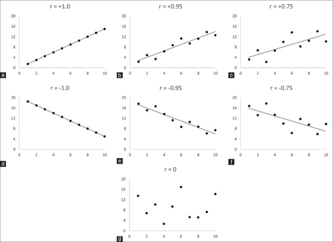
Two variables are said to be “positively” correlated [Figure 1a-c] when their values change in tandem, i.e., increasing values of one are associated with increasing values of the other. By contrast, a “negative” correlation [Figure 1d-f] exists when increasing values of one variable are associated with a decrease in the values of the other. Variables with no or little discernible relationship [Figure 1g] are said to have “no correlation.”

Figure 1.

Scatter plots of relationship between values of two quantitative variables and their corresponding correlation coefficient (r) values. “r” can vary between − 1.0 and + 1.0. If as the values of one variable (say on X-axis) increase, those of the other variable (on Y-axis) increase, “r” is positive (a-c); however, if the latter decrease, “r” is negative (d-f). When the values of two variables have no clear relation, “r” is zero (g). The absolute values of “r” are higher when the individual data points are closer to a line showing the linear trend (a > b > c; d > e > f)

Magnitude

The absolute value of r represents the strength of association. A value of 1.0 implies a perfect linear relationship between the two variables, i.e., all observations lie on a straight line [Figure 1a and d], whereas 0 indicates the absence of any linear relationship [Figure 1g]. Higher values (closer to 1.0) imply that individual observations lie close to an imaginary line describing the relationship between the two variables [Figure 1b and e], and lower values imply that the observations are more spread out [Figure 1c and f].

INTERPRETATION OF VALUE OF CORRELATION COEFFICIENT

Square of correlation coefficient (r²), known as coefficient of determination, represents the proportion of variation in one variable that is accounted for by the variation in the other variable. For example, if height and weight of a group of persons have a correlation coefficient of 0.80, one can estimate that 64% (0.80 × 0.80 = 0.64) of variation in their weights is accounted for by the variation in their heights.

It is possible to calculate P value for an observed correlation coefficient to determine whether a significant linear relationship exists between the two variables of interest or not. However, with medium- to large-sized samples, these methods show even small correlation coefficients to be highly significant and hence their use is generally eschewed.

WHEN SHOULD CORRELATION NOT BE USED?

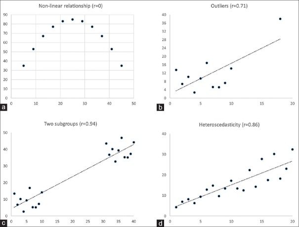
• The correlation coefficient looks for a linear relationship. Hence, it can be fallacious in situations where two variables do have a relationship, but it is nonlinear. For instance, hand-grip strength initially increases with age (through childhood and adolescence) and then declines (e.g., Figure 2a). In such cases, “r” could be low (r = 0 for the data in Figure 2a), even though there is a clear relationship.

• Correlation analysis assumes that all the observations are independent of each other. Thus, it should not be used if the data include more than one observation on any individual. For instance, in the above example, if hand-grip strength had been measured twice in some subjects that would be an additional reason not to use correlation analysis.

• If one (or a few) individual observation in the sample is an outlier, i.e., located far away from the others, it may introduce a false sense of relationship [Figure 2b]. Please note that the data points in this figure are identical to those in Figure 1g, except for the addition of one outlier. On excluding this outlier, the value of r would drop from 0.71 to 0!

• If the dataset has two subgroups of individuals whose values for one or both variables differ from each other [Figure 2c], this can lead to a false sense of relationship overall, even when none exists within each subgroup. For instance, let us consider a group of 20 men and 20 women. If one plots their heights (on X-axis) and hemoglobin levels (on Y-axis), most women may end up in the left lower corner (shorter and lower hemoglobin) and most men in the right upper corner (taller and higher hemoglobin), suggesting a false relationship (a positive “r” value) between height and hemoglobin levels.

• With very small sample size (say 3–6 observations), a relationship may appear to be present even though none exists.

• Linear correlation analysis applies only to data on a continuous scale. It should not be used when one or both variables have been measured using an ordinal scale, for example, patients’ assessment of pain severity on a scale of 0–10, where higher number means worse pain but similar differences (say from 1 to 3 and from 6 to 8) do not necessarily imply similar change in pain. In these cases, a Spearman's rank correlation method should be used.

• Relationship between a variable and one of its components (e.g., aggregate marks vs. marks in one subject). For instance, it would be fallacious to use correlation to assess the relationship of height of a group of persons with the lengths of their body's lower segments since the lower segment forms a part of the overall height.

• Heteroscedasticity or a situation in which the one variable has unequal variability across the range of values of a second variable. For instance, if one looks at the relationship of annual health expenditure versus the annual income of a family, the former is likely to vary more for richer persons than for poor persons [Figure 2d].

Figure 2.

Situations in which linear correlation should not be used: (a) two variables have a relationship which is nonlinear (analysis of data points in this figure shows r = 0, thus failing to detect the relationship), (b) the data have one or a few outliers (one outlier at right upper end resulted in a false relationship with r = 0.71; exclusion of this point reduces r to near zero), (c) when the data have two subgroups, within each of which there is no correlation, and (d) when variability in values on Y-axis changes with values on X-axis. Each situation is described further in the text

Many of the above pitfalls are easily avoided if one first makes a scatter plot for the data and visually inspects it for nonlinear relationships, outliers, or presence of obvious subgroups.

In addition, correlation analysis is also often inappropriately used to measure agreement between two methods of measuring the same thing (e.g., tumor volume measured using ultrasound and computed tomography). This will be discussed in the next article in this series.

A FINAL CAUTION: CORRELATION DOES NOT MEAN CAUSATION

A relationship between two variables is sometimes taken as evidence that one causes the other. This is, however, often not true, and hence the popular statistical adage: “Correlation does not imply causation.” You may wish to visit https://en.wikipedia.org/wiki/Correlation_does_not_imply_causation for some interesting insights into how correlation can arise without any causative link.

Examples of such noncausative correlation include (i) countries’ annual per capita chocolate consumption and the number of Nobel laureates per 10 million population;[1] (ii) weekly ice-cream consumption and a number of drowning incidents in swimming pools. These are due to the association of both the variables being studied to national income[2] and hot weather, respectively.

ENDPIECE

Correlation analysis is a very powerful tool to explore relationships in data. However, one must be careful to use it only when it is applicable. Many of these problems can be avoided by a careful thought about the data, plotting the raw data (to look for nonlinear relationships, outliers, and heteroscedasticity of data), and by thinking in terms of coefficient of determination in preference to the correlation coefficient.

Financial support and sponsorship

Nil.

Conflicts of interest

There are no conflicts of interest.

REFERENCES

- 1.Messerli FH. Chocolate consumption, cognitive function, and Nobel laureates. N Engl J Med. 2012;367:1562–4. doi: 10.1056/NEJMon1211064. [DOI] [PubMed] [Google Scholar]
- 2.Maurage P, Heeren A, Pesenti M. Does chocolate consumption really boost Nobel Award chances? The peril of over-interpreting correlations in health studies. J Nutr. 2013;143:931–3. doi: 10.3945/jn.113.174813. [DOI] [PubMed] [Google Scholar]