Hot Spots Conjecture and Its Application to Modeling Tubular Structures

Abstract

The second eigenfunction of the Laplace-Beltrami operator follows the pattern of the overall shape of an object. This geometric property is well known and used for various applications including mesh processing, feature extraction, manifold learning, data embedding and the minimum linear arrangement problem. Surprisingly, this geometric property has not been mathematically formulated yet. This problem is directly related to the somewhat obscure hot spots conjecture in differential geometry. The aim of the paper is to raise the awareness of this nontrivial issue and formulate the problem more concretely. As an application, we show how the second eigenfunction alone can be used for complex shape modeling of tubular structures such as the human mandible.

1 Introduction

The second eigenfunction of the Laplace-Beltrami operator is drawing significant attention in recent years mainly as a tool for extracting shape features in high dimensional data [2,8,10]. The gradient of eigenfunction tends to follow the pattern of the overall shape of data and has been used to establish the intrinsic coordinate system of the data. This geometric property has been well known and often been used in computer vision and medical imaging applications. The second eigenfunction of the graph Laplacian was used to construct the Laplacian eigenmaps for low dimensional embedding [2]. The critical points of the second eigenfunction were used as anatomical landmarks for piecewise registration of colon surfaces [8]. The Reeb graph of the second eigenfunction was used in characterizing hippocampus shape [10].

All these studies rely on the geometric property of the second eigenfunction and somehow captures the overall shape of data. However, this property has not been mathematically formulated precisely. In fact, it is related to an obscure conjecture called the hot spots conjecture in differential geometry [1]. In this paper, we will explore the issue in detail and formulate the geometric property more precisely, which will be illustrated with examples and a proof for simple shape.

2 The Second Laplace-Beltrami Eigenfunction

Second Eigenfunction

The eigenfunctions of the Laplace-Beltrami operator has been used in many different contexts in image analysis [8,9,10]. Eigenfunctions ψ_j of Laplace-Beltrami operator Δ in ℳ satisfy Δψ_j = λ_jψ_j. The eigenfunctions form an orthonormal basis in ℳ. We can order the eigenfunctions ψ₀, ψ₁, ψ₂, ⋯ corresponding to the increasing order of eigenvalues 0=λ₀ ≤ λ₁ ≤ λ₂ ≤⋯.Other than ${\psi }_0=1/\sqrt{\mu (M)}$, close form expression for other eigenfunctions are unknown. However, using the cotan discretization for the Laplace-Beltrami operator [3,9], we can obtain the eigenfunctions numerically. The MATLAB code is available at http://brainimaging.waisman.wisc.edu/~chung/lb.

The critical point of the second eigenfunction ψ₁ usually occur at the two extremes of an elongated object (Figure 1). So the gradient of the second eigenfunction follows the shape of elongated objects. In computer vision literature, this monotonicity property was observed but without any mathematical justification [2,10]. Many treated it as a proven fact although the underlying conjecture has yet to be proved [1].

Fig. 1.

The second eigenfunction ψ₁ for different mandible surfaces. The second eigenfunction for an elongated closed object is a smooth monotonic function increasing from one tip of surface to the other tip of the surface.

Conjecture 1

(Rauch’s hot spots conjecture) [1] Let ℳ be an open connected bounded subset. Let f (σ, p) be the solution of heat equation

$$\frac{\partial f}{\partial \sigma }=\mathrm{\Delta }f$$ (1)

with the initial condition f (0, p) = g(p) and the Neumann boundary condition $\frac{\partial f}{\partial n}\left(\sigma ,p\right)=0$ on the boundary ∂ℳ. Then for most initial conditions, if p_hot is a point at which the function f (·, p) attains its maximum (hot spot), then the distance from p_hot to ∂ℳ tends to zero as σ → ∞ [1].

We can also claim a similar statement for minimum (cold spots) as well. Conjecture 1 basically implies that the hot and cold spots move away from the origin toward the boundary as the diffusion continues. Note that the solution to heat equation (1) is given by heat kernel expansion [9]:

$$K_{\sigma }\ast g(p)={\displaystyle \sum _{j=0}^{\infty }{e}^{-{\mathrm{\lambda }}_j\sigma }}{\beta }_j{\psi }_j(p),$$ (2)

where β_j = 〈ψ_j, g〉 are Fourier coefficients. Since λ₀ = 0 and ${\psi }_0=1/\sqrt{\mu (ℳ)}$, we have

$$K_{\sigma }\ast g(p)=\frac{{\displaystyle {\int }_{ℳ}g(p)d\mu (p)}}{\mu \left(ℳ\right)}+{\beta }_1{e}^{-{\mathrm{\lambda }}_1\sigma }{\psi }_1(p)+R(\sigma ,p),$$ (3)

where the first term is the average signal and the remainder R goes to zero faster than $e^{-{\mathrm{\lambda }}_1\sigma }$ as σ → ∞ [1]. Therefore, the behavior of the propagation of the hot spots is basically governed by the eigenfunction ψ₁.

What will happen if there is no boundary? In the case of closed manifold with no boundary, the Neumann boundary condition simply disappears so the direct application of the hot spots conjecture is not valid. Since ψ₁ asymptotically behaves like the heat equilibrium state, hot and cold spots cannot possibly be located in close proximity. Thus, we propose the following conjecture.

Conjecture 2

For a closed and sufficiently smooth simply connected surface ℳ with no boundary, the geodesic distance d between any two points p and q is bounded by

$$d(p,q)\le d(p_{\mathit{min}},p_{\mathit{max}}).$$

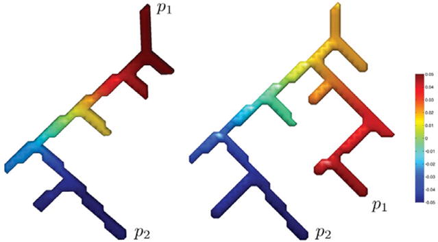
Conjecture 2 implies that the hot and cold spots give the maximum possible geodesic distance among all possible pairs of points and define the direction of elongation of data. Figure 2 illustrates Conjecture 2. For any complicated branching binary tree structures like Figure 2, the hot and cold spots occur at the two extreme points along the longest geodesic path. The hot spots conjecture basically dictates that it is possible to find the maximum possible geodesic path by simply finding the critical points in the second eigenfunction. Conjecture 2 can be applicable not only to differentiable manifolds but to graphs and surface meshes as well.

Fig. 2.

The second eigenfunction ψ₁ of branching tubular structures. The maximum (p₁) and the minimum (p₂) of ψ₁ always occur at the points of maximum geodesic distance.

3 Hot Spots Conjecture Applied to Fiedler’s Vector

Surface meshes can be considered as graphs. The connection between the eigenfunctions of continuous and discrete Laplacians has been well established by many authors [6,11]. Many properties of eigenfunctions of the Laplace-Beltrami operator have discrete analogues. The second eigenfunction of the discrete graph Laplacian is called the Fiedler vector and it has been studied in connection to the graph and mesh processing, manifold learning and the minimum linear arrangement problem [5] Let G = {V, E} be the graph with the vertex set V and the edge set E. G is the discrete approximation of the underlying continuous manifold ℳ. We will simply index the node set as V = {1, 2, ⋯, n}. If two nodes i and j form an edge, we denote it as i ~ j. Various forms of graph Laplacian have been proposed but many graph or discrete Laplacian L = (l_ij) is a real symmetric matrix of the form

$$l_{ij}=(\begin{array}{cc}-w_{ij},& i\sim j\\ {\displaystyle {\sum }_{i\ne j}{w}_{ij},}& i=j\\ 0,& \text{otherwise}\end{array}$$

for some edge weight w_ij. The graph Laplacian L can be decomposed as L = D − W, where D = (d_ij) is the diagonal matrix with $d_{ii}={\displaystyle {\sum }_{j=1}^n{w}_{ij}}$ and W = (w_ij). For a vector f = (f₁, ⋯, f_n)′ observed at the n nodes, the discrete analogue of the Dirichlet energy is given by

$$ℰ(f)=\mathbf{f}\prime L\mathbf{f}={\displaystyle \sum _{i,j=1}^n{w}_{ij}{(f_i-f_j)}^2={\displaystyle \sum _{i\sim j}{w}_{ij}}}{(f_i-f_j)}^2\cdot$$ (4)

The Fiedler’s vector f = (f₁, ⋯, f_n)′ is obtained as the minimizer of the quadratic polynomial ψ₁ = arg min_f ℰ(f) subject to the quadratic constraint ${\Vert \mathbf{f}\Vert }^2={\displaystyle {\sum }_i{f}_i^2}=1.$ The Dirichlet energy measures the smoothness of f so the second eigenfunction should be the smoothest possible map among all possible functions. Since ψ₁ is required to be orthonormal with ψ₀, we also have an additional constraint ${\displaystyle {\sum }_i{f}_i=0.}$ Therefore, ψ₁ is positive on half of ℳ and negative on the other half. However, it still does not explicitly tell us that a smooth function has to be monotonically changing from one end to the other.

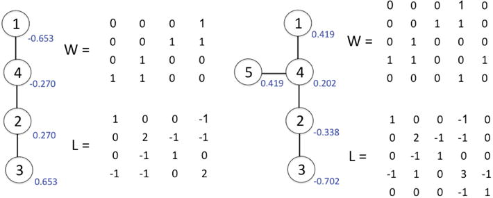
The constraints force ψ₁ to have at least two differing sign domains in which ψ₁ has one sign. The nodal set of eigenfunctions ψ_i is defined as the zero level set ψ_i(p) = 0. Then Courant’s nodal line theorem states that the nodal set of the i-th eigenfunction ψ_i−1 divide the manifold into no more than i sign domains [4,6,11]. Hence, the second eigenfunction must have exactly 2 disjoint sign domains. At the positive sign domain, we have the global maximum and at the negative sign domain, we have the global minimum. This is illustrated in Figure 3 and 4. Although it is difficult to prove the general statement, the conjecture can be proven for specific cases. Here we provide a first heuristic proof for a path, which is a graph with maximal degree 2 and without a cycle.

Fig. 3.

A graph, the weights W and the graph Laplacian L. The weights are simply the adjacency matrix. The second eigenfunction ψ₁ value is displayed in blue. (a) This example is given in [7]. The maximum geodesic distance is obtained between the nodes 1 and 3, which are also hot and cold spots. (b) In this example, there are two hot spots 1 and 5 which correspond to two maximal geodesic paths 1-4-2-3 and 5-4-2-3.

Fig. 4.

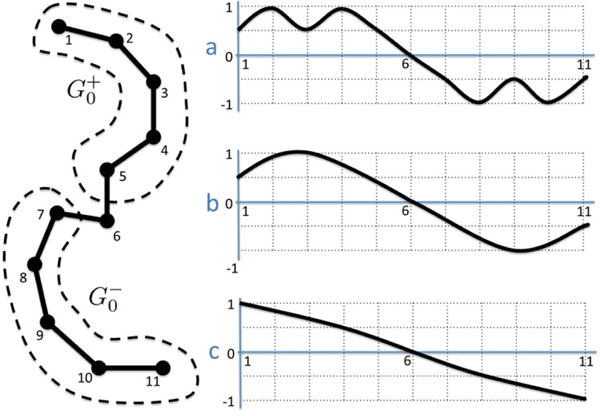
A path with positive $(G_0^{+})$ and negative $(G_0^{-})$ sign domains. Among many possible candidate functions, (a) and (b) are not tight so they can’t be the second eigenfunctions.

Tightness

For a function f defined on the vertex set V, let $G_s^{-}$ be the subgraph induced by the vertex set $V_s^{-}=\{i\in V|f_i<s\}.$ Similarly, let $G_s^{+}$ be the subgraph induced by the vertex set $V_s^{+}=\{i\in V|f_i>s\}.$ For any s, if $G_s^{-}$ and $G_s^{+}$ are either connected or empty, then f is tight [11]. The concept of tightness is crucial in proving the statement. When s = 0, $G_0^{+}$ and $G_0^{-}$ are sign graphs. If we relax the condition so that $G_s^{+}$ contains nodes satisfying f_i ≥ s, we have weak sign graphs. The second eigenfunction on a graph with maximal degree 2 (either cycle or path) is tight [11]. Figure 4 shows an example of a path with 11 nodes. Among three candidates for the second eigenfunction, (a) and (b) are not tight while (c) is. Note that the candidate function (a) has two disjoint components when thresholded at s = 0.5 so it cannot be tight. In order to be tight, the second eigenfunction cannot have a positive minimum or a negative maximum at the interior vertex in the graph [6]. This implies that the second eigenfunction must decrease monotonically from the positive to negative sign domains as shown in (c) and have the critical points at the two end points. This has to be true for a general case as well.

4 Application: Mandible Growth Modeling

The CT imaging data set consists of 76 mandibles (40 males and 36 females). The age distribution was 11.33±5.60 years for the females, and 9.54±5.71 years for the males. The image acquisition and processing details for acquiring the mandible surface meshes are given in [9].

Features

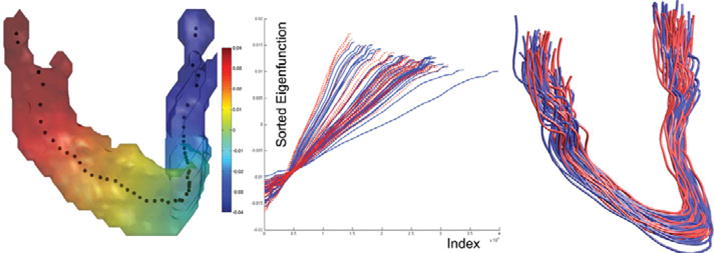
In most literature dealing with the eigenfunctions of the Laplace-Beltrami operator, the whole spectrum of eigenvalues or eigenfunctions were used for shape analysis [9,10]. Here, we show how the second eigenfunction alone can be used as the shape feature. Once we obtained the second eigenfunctions for all subjects, we sorted them in increasing order (Figure 5). The sorted eigenfunctions are almost straight lines. A bigger mandible (more indices) exhibits a less steeper slope. Therefore, the rate of increase of the sorted eigenfunction (slope of linear fit) can be used for characterizing subject anatomical variability.

Fig. 5.

Left: The centroids of level contours of the 2nd eigenfunction. Middle: The sorted second eigenfunctions (female =red, male = blue). Right: The centerlines of all 76 subjects showing the proper alignment.

General Linear Models

We examined how the rate of increase can be used in characterizing the growth of the mandible. We used the general linear model (GLM) of the form <monospace>feature</monospace> = β₀ + β₁ <monospace>gender</monospace> + β₂ <monospace>age</monospace> + ε The parameters are estimated using the least squares method and the statistical significance is determined using the F-statistic. There is weakly significant gender difference (β₁) (p-value = 0.08) and highly significant age effect (β₂) (p-value < 10⁻⁷) for the rate of increase. We conclude that the mandible size grows at a much faster rate for males than females.

References

- 1.Banuelos R, Burdzy K. On the Hot Spots Conjecture of J Rauch. Journal of Functional Analysis. 1999;164:1–33. [Google Scholar]
- 2.Belkin M, Niyogi P. Laplacian eigenmaps and spectral techniques for embedding and clustering. Advances in Neural Information Processing Systems. 2002;1:585–592. [Google Scholar]
- 3.Chung MK, Taylor J. Diffusion smoothing on brain surface via finite element method. Proceedings of IEEE International Symposium on Biomedical Imaging (ISBI) 2004;1:432–435. [Google Scholar]
- 4.Courant R, Hilbert D. Methods of Mathematical Physics, english edn. Interscience; New York: 1953. [Google Scholar]
- 5.Fiedler M. Algebraic connectivity of graphs. Czechoslovak Mathematical Journal. 1973;23:298–305. [Google Scholar]
- 6.Gladwell GML, Zhu H. Courant’s nodal line theorem and its discrete counterparts. The Quarterly Journal of Mechanics and Applied Mathematics. 2002;55:1–15. [Google Scholar]
- 7.Hall KM. An r-dimensional quadratic placement algorithm. Management Science. 1970;17:219–229. [Google Scholar]
- 8.Lai Z, Hu J, Liu C, Taimouri V, Pai D, Zhu J, Xu J, Hua J. Intrapatient supine-prone colon registration in CT colonography using shape spectrum. In: Jiang T, Navab N, Pluim JPW, Viergever MA, editors. MICCAI 2010 LNCS. Vol. 6361. Springer; Heidelberg: 2010. pp. 332–339. [DOI] [PubMed] [Google Scholar]
- 9.Seo S, Chung MK, Vorperian HK. Heat kernel smoothing using laplace-beltrami eigenfunctions. In: Jiang T, Navab N, Pluim JPW, Viergever MA, editors. MICCAI 2010 LNCS. Vol. 6363. Springer; Heidelberg: 2010. pp. 505–512. [DOI] [PMC free article] [PubMed] [Google Scholar]
- 10.Shi Y, Lai R, Krishna S, Sicotte N, Dinov I, Toga AW. Anisotropic Laplace-Beltrami eigenmaps: Bridging Reeb graphs and skeletons. Proceedings of Mathematical Methods in Biomedical Image Analysis (MMBIA) 2008:1–7. doi: 10.1109/CVPRW.2008.4563018. [DOI] [PMC free article] [PubMed] [Google Scholar]
- 11.Tlusty T. A relation between the multiplicity of the second eigenvalue of a graph laplacian, courants nodal line theorem and the substantial dimension of tight polyhedral surfaces. Electrnoic Journal of Linear Algebra. 2007;16:315–324. [Google Scholar]