Prediction of lung cancer incidence on the low-dose computed tomography arm of the National Lung Screening Trial: A dynamic Bayesian network

Abstract

Introduction

Identifying high-risk lung cancer individuals at an early disease stage is the most effective way of improving survival. The landmark National Lung Screening Trial (NLST) demonstrated the utility of low-dose computed tomography (LDCT) imaging to reduce mortality (relative to x-ray screening). As a result of the NLST and other studies, imaging-based lung cancer screening programs are now being implemented. However, LDCT interpretation results in a high number of false positives. A set of dynamic Bayesian networks (DBN) were designed and evaluated to provide insight into how longitudinal data can be used to help inform lung cancer screening decisions.

Methods

The LDCT arm of the NLST dataset was used to build and explore five DBNs for high-risk individuals. Three of these DBNs were built using a backward construction process, and two using structure learning methods. All models employ demographic, smoking status, cancer history, family lung cancer history, exposure risk factors, comorbidities related to lung cancer, and LDCT screening outcome information. Given the uncertainty arising from lung cancer screening, a cancer state-space model based on lung cancer staging was utilized to characterize the cancer status of an individual over time. The models were evaluated on balanced training and test sets of cancer and non-cancer cases to deal with data imbalance and overfitting.

Results

Results were comparable to expert decisions. The average area under the curve (AUC) of the receiver operating characteristic (ROC) for the three intervention points of the NLST trial was higher than 0.75 for all models. Evaluation of the models on the complete LDCT arm of the NLST dataset (N = 25, 486) demonstrated satisfactory generalization. Consensus of predictions over similar cases is reported in concordance statistics between the models’ and the physicians’ predictions. The models’ predictive ability with respect to missing data was also evaluated with the sample of cases that missed the second screening exam of the trial (N = 417). The DBNs outperformed comparison models such as logistic regression and naïve Bayes.

Conclusion

The lung cancer screening DBNs demonstrated high discrimination and predictive power with the majority of cancer and non-cancer cases.

1. Introduction

Lung cancer is the leading cause of cancer death worldwide. In the United States, it is estimated to be responsible for over 150,000 annual deaths [1, 2], comprising 27% of all cancer deaths [3, 4]. A number of factors have been associated with the high incidence and mortality of lung cancer, the most important being cigarette smoking [5]; and late-stage/advanced diagnoses [6], wherein treatment is non-curative. Patients with lung cancer have a higher probability of metastases and a relatively low 5-year survival rate of 18% [7]. Markedly, when diagnosed early, the 5-year survival rate increases to 54%. However, only 15% of all lung cancer cases are detected at an early stage [7]. Considering the high mortality associated with late-stage lung cancer diagnosis, it is crucial that patients who are at high risk of lung cancer be identified and monitored so that early treatment can be initiated if needed.

Screening has the potential to detect the formation of problematic pulmonary nodules at an early stage; and when detected earlier, more choices for treatment are available, along with improved chances of survival. Evidence regarding the benefits of lung screening comes from the landmark National Lung Screening Trial (NLST), which demonstrated a 20% mortality reduction in lung cancer in individuals who underwent screening using low-dose computed tomography (LDCT) relative to plain chest radiography [8]. Given this evidence, the American Patient Protection and Affordable Care Act (ACA) has mandated that CT screening be covered by private insurers; the Centers for Medicare and Medicaid Services (CMS) has also approved reimbursement of CT screening in Medicare-eligible patients up to the age of 77. Unfortunately, LDCT also detects many benign nodules and non-cancer related pathologies (e.g., inflammation, emphysema, other lesions), resulting in many false positives and the need for further diagnostic evaluation to confirm findings. In fact, the false positive rate of screening strategies used by the NLST was determined to be over 23% for individuals that underwent additional diagnostic imaging [8]. Confirmed cancer cases in the NLST CT positive arm were determined to be 3.6% of all cases and any lung cancer detected had a probability of 18.5% to be an over-diagnosis [9]. This suggests that while an acceptable false negative rate is achieved, the majority of healthy patients in a population get over-screened and/or over-diagnosed. Unnecessary diagnostic procedures, such as biopsies and thoracotomies, place healthy patients at a higher risk of complications and incur an unnecessary psychological burden [10]. A framework that optimizes early detection while reducing false negative rates would be ideal, and can then be used to support more individually-tailored screening recommendations.

This work aims to provide insights into how recommendations can be individualized over time in the context of lung cancer screening. We explore the issues surrounding the development and evaluation of a dynamic Bayesian network (DBN), built from the NLST dataset, to predict the development of lung cancer in high-risk patients. We compare DBNs built using the “backward construction” method and “learned” DBNs¹. We also compare and contrast the DBNs’ performance versus experts and other predictive models for lung cancer. Relative to existing predictive models, our methodology has several advantages. First, it can make sensible predictions even with missing data, a common occurrence in real-world settings (e.g., a missed screening exam). Second, it is built on top of a lung cancer state-space defined on lung cancer staging. This state space unites lung cancer risk factors and diagnostic procedures in a meaningful network structure, while also enabling the flow of probabilistic influence between these variables. Third, contrary to existing predictive methods for lung cancer screening, our methodology and in particular DBNs can explain and show the contributing factors for its predictions (i.e., factors investigated in lung cancer screening). We present the results of our evaluations and discuss the advantages and limitations of our work, providing some future directions for further improvement.

2. Background

In recent years, many risk models have been published to predict the development of different cancers [11]. In lung cancer, Bach et al. [12] developed an analog of the well-known Gail model used to calculate the risk for developing breast cancer [13, 14]. The model predicts the 10-year probability of an individual being diagnosed with lung cancer. This 10-year risk was obtained through the use of two one-year risk models, a lung cancer diagnosis model and a competing model of dying without lung cancer. Subsequently, the one-year models were run recursively over 10 epochs (i.e., years) to obtain cumulative probabilities over time [15]. Even though the model does not distinguish the risks of the various types of lung cancer, it can identify those subjects who are most likely to develop lung cancer [12]. The model’s validity was assessed by Conin et al. [16] using 6,239 smokers from the placebo arm of the Alpha-Tocopherol, Beta-Carotene Cancer Prevention (ATBC) Study. The risk and competing risk models both underestimated the observed lung cancer risk and the observed non-lung cancer mortality risk for individuals that smoked less than 20 cigarettes per day. Raji et al. [17] evaluated the predictive accuracy of the Liverpool Lung Project Risk Model. This single log-odds model, developed through the use of logistic regression, was developed from the Liverpool Lung Project Cohort (LLPC) [15] study. The model was evaluated in three independent external datasets, from Europe and North America, with good discrimination in all three datasets. The area under the curve (AUC) in these datasets varied from 0.67–0.82 [17]. Spitz et al. [18] developed a lung cancer risk prediction model using a multivariate regression analysis to develop log-odds models for never, current, and former smokers. The model’s concordance statistics (0.57, 0.63 and 0.58, respectively) and discriminatory ability (true positive rates in high-risk groups of current and former smokers were 0.69 and 0.70, respectively [18]) were satisfactory, but precision was modest [19]. Finally, more recently, Tammemagi et al. [20] developed lung cancer models that demonstrated high discrimination and calibration using the Prostate, Lung, Colorectal and Ovarian Cancer (PLCO) Screening Trial. In contrast with most lung cancer prediction studies, this study’s models incorporated a wider range of risk factors that were incrementally evaluated using AUC as a comparison metric. The models were evaluated for the prediction of lung cancer on the entire PLCO dataset and a subset of ever-smokers, with both models achieving an AUC of 0.857 and 0.841, for the PLCO dataset, and 0.805 and 0.784, for the ever-smokers subset, respectively.

The models we describe for lung cancer screening are based on a dynamic Bayesian network. DBNs, as well as Bayesian networks (BNs), are increasingly being used in clinical screening and treatment decision making. For example, DBNs and BNs have been used in the domain of nosocomial infections [21], pneumonia [22], cardiac surgery [23], gait analysis [24], osteoporosis [25], oral cancer [26], colon cancer [27], cervical cancer [28], and breast cancer [29, 30, 31, 32]. Notably, [33] proposed a Bayesian network for lung cancer built from both physical and biological data (biomarkers) for the prediction of local failure in non-small cell lung cancer (NSCLC) after radiotherapy. This integrated approach was tested on two different NSCLC datasets with the biological data contributing the most in the model’s performance. In this study, to handle the inherent temporal nature of screening observations over time, we propose a set of DBNs to obtain individualized predictions for patients at high-risk for lung cancer. In the following sections, we present the methodology as well as the theoretical formulations supporting our model.

3. Methods

We used the NLST dataset to create DBNs for the prediction of lung cancer incidence. The description of the dataset, overall methods, measured outcomes, and statistical evaluation methods used in this study are as follows.

3.1. The NLST dataset

The NLST is a randomized, multi-site trial that examined lung cancer-specific mortality among participants in an asymptomatic high-risk cohort. Subjects underwent screening with the use of low-dose CT or a chest x-ray. Over 53,000 participants each underwent three annual screenings from 2002–2007 (approximately 25,500 in the LDCT study arm), with follow-up post-screening through 2009. Lung cancers identified as pulmonary nodules were confirmed by diagnostic procedures (e.g., biopsy, cytology); participants with confirmed lung cancer were subsequently removed from the trial for treatment.

The NLST dataset provides a longitudinal perspective on high-risk lung cancer patients in terms of demographics, clinical history, and imaging data. We used subjects from the LDCT arm, across all three screening events and the post-screening period of the trial. Information used in our study includes: demographics (e.g., age, gender, body mass index); smoking history; family history of cancer; personal history of cancer; history of comorbidities related to lung cancer; occupational exposures (e.g., asbestos, coal, chemicals); and LDCT screening outcomes. Table 1 summarizes the number of cases determined to have cancer during any of the three imaging points of intervention (and the remaining number of non-cancer patients), as well as post-screening cancer patients (i.e., those individuals who went on to develop lung cancer after the third screening event).

Table 1.

NLST dataset, detailing the determined health state of a subject after each screening exam. Post-trial cancer cases represent the cancer cases that lung cancer was the cause of their death and were not identified as lung cancer cases through the NLST trial. The number of patients shown represent the patients for which we have information about the development of lung cancer. A cancer incidence occurring after the first screening and before the second screening was assumed to be a first screening cancer. A cancer incidence occurring after the second screening and before the third screening was assumed to be a second screening cancer. A cancer incidence occurring after the third screening and before the post screening period was assumed to be a third screening cancer. The above information was computed from the NLST dataset under our possession.

	First Screening	Second Screening	Third Screening	Post-screening	Post-trial	Total Cases
Remaining non-cancer subjects	25,530	25,217	24,842	24,477	24,461	-
Individuals with confirmed cancer	305	174	223	365	16	1,083
Deceased subjects	11	139	152	-	-	302
Total subjects	25,846	25,530	25,217	24,842	24,477	-

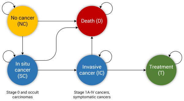
Based on the true state of each patient (i.e., cancer or non-cancer) we designed a simplified state space model representing the “ground truth” disease state of each patient, after each screening time point. Figure 1 represents the state-space and the allowed transitions through these states. No-Cancer (NC) is the state in which the individual has no abnormalities or has abnormalities that are not suspicious for lung cancer (e.g., lung nodules smaller than 4 mm). The In Situ-Cancer (SC) state captures an individual who has abnormalities suspicious for lung cancer (e.g., findings larger than 4 mm). In terms of lung cancer staging, the SC state captures Stage 0 and occult carcinoma stages [34]. The Invasive-Cancer (IC) state represents individuals with confirmed diagnoses of cancer through the use of additional diagnostic procedures (e.g., biopsy). The IC state captures Stage IA–IV lung cancers. The Treatment state represents the state in which the individual was confirmed with cancer and is receiving treatment. Lastly, the Death state indicates an individual who is deceased, either from the cancer (without treatment) or due to some other cause. From this state model, the three cancer-related states (NC, SC, IC) were used to represent discrete characterizations for a given patient’s likelihood of cancer following screening observations over time.

Figure 1.

The underlying disease state space model for lung cancer used in this study, modeled after the process flow in the NLST. The arrows depict allowed transitions in the state space. In the Non-Cancer state, where everyone starts, the individual has no abnormalities or abnormalities smaller than 4 mm. In the In Situ Cancer state the individual has abnormalities larger than 4 mm, which are not confirmed to be cancerous. In the Invasive Cancer state the individual is confirmed to have cancer through the use of diagnostic procedures, such as biopsy. In the Treatment state the individual is receiving care for the cancer, and is removed from the screening process. Finally, in the Death state the individual is deceased. The process described in this study terminates when an individual enters the Death or the Treatment state. The transition from the Treatment to the Death state is not depicted here as we only focus at the process of identifying an individual with lung cancer (e.g., an individual with invasive cancer whose process ends when the individual enters the Death or Treatment state).

3.2. Dynamic Bayesian networks

A dynamic Bayesian network is a model that repeats the static interactions of a conventional Bayesian network over time [35]. In DBNs, we represent a joint probability distribution over temporal trajectories that specify the assignment of values to each random variable $X_i^{(t)}$ at different time points t. A DBN follows the Markov assumption in which the future state of the system only depends on the current state of the system and is independent of the past. Thus, in the case of a DBN, which is an unrolled Bayesian network, the random variable X_i of the network will depend only on its parents, Par(X_i).

$$P(X_1,\dots ,X_n)=\prod _{i=1}^{n}P(X_i\mid \mathit{Par}(X_i)).$$ (1)

The structure and the probabilities P(X^(t+1)|X^(t)) can be assumed the same for all t (i.e., time invariant). Such a system is a stationary dynamical system. In this case the model can consist of two parts [36]:

1. A prior model that specifies the initial distribution of the process:

   $$P(X^{(0)})=\prod _{X^{(0)}\in {\mathbf{X}}^{(\mathbf{0})}}P(X^{(0)}\mid \mathit{Par}(X^{(0)}))$$ (2)
2. A transition model that specifies the evolution of the process across time points:

   $$P(X^{(t+1)}\mid X^{(t)})=\prod _{X^{(t+1)}\in {\mathbf{X}}^{(\mathbf{t}+\mathbf{1})}}P(X^{(t+1)}\mid \mathit{Par}(X^{(t+1)})).$$ (3)

A DBN can be used to estimate conditional distributions through the use of the chain rule for Bayesian networks. This ability was used in our lung cancer screening DBN to obtain the probability of a positive outcome of a biopsy for a given individual. Equation 4 represents the conditional probability of variable $X_i^{(t)}$ given evidence about certain random variables X = {X₁, ..., X_n−1} in the network structure.

$$P(X_i^{(t)}\mid \mathbf{X})=\prod _{t\in T}\prod _{i=1}^{n}P(X_i^{(t)}\mid \mathit{Par}(X_i^{(t)})).$$ (4)

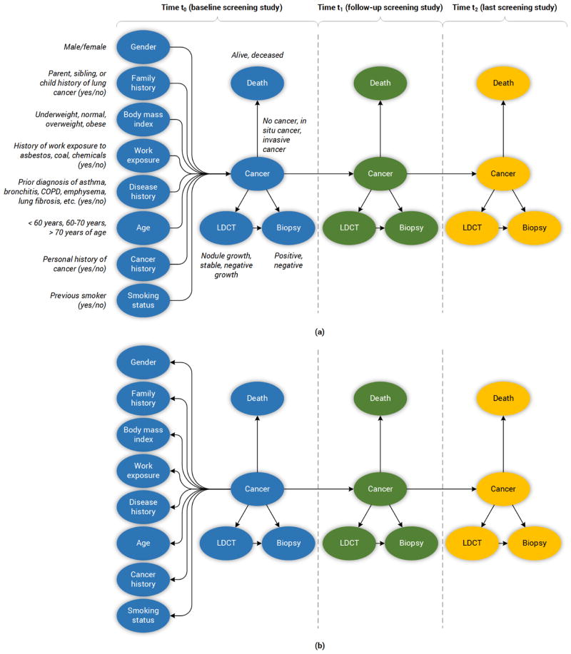
An example of the computation of the probability of the Biopsy outcome on a patient at the second screening (t = 1) based on the networks in Figure 2 is shown below. The computation of the conditional probability is based on the evidence of the individual on the variables of the model:

$$\begin{array}{c}\mathrm{P}({\text{Biopsy}}^{(1)}\mid \text{Gender}=\mathbf{Female},\text{Family}\text{History}=\mathbf{Yes},\text{Body}\text{Mass}\text{Index}=\mathbf{Obese},\text{Work}\text{Exposure}=\mathbf{Yes},\\ \text{Disease}\text{History}=\mathbf{Yes},\text{Age}=\mathbf{64},\text{Cancer}\text{History}=\mathbf{No},\text{Smoking}\text{Status}=\mathbf{Yes}).\end{array}$$

Figure 2.

The diagram above depicts the structure of the lung cancer screening DBNs. Italicized text indicates the discreted states considered per variable. (a) The Forward-Arrow DBNs. (b) The Reversed-Arrow DBN. The total number of epochs in both models is 3.

3.3. The lung cancer screening DBNs

Deriving a DBN broadly involves two steps. First, deriving the structure (i.e., a directed acyclic graph); and second, parameterizing the network structure (i.e., estimating the probabilities for the CPTs of the network). In this work, we used the NLST dataset to build five different variations of networks: three expert-driven DBNs (“backward construction”) and two DBNs derived from structure learning methods. Specifically, the models are as follows:

• The expert-driven DBNs consist of two Forward-Arrow DBNs (see Figure 2a) and one Reversed-Arrow DBN (Model B, see Figure 2b): 1) a Forward-Arrow DBN using a NoisyMax gate (Model A) for parameter reduction of the Cancer node, and for comparison, 2) a Forward-Arrow DBN without a NoisyMax gate (Model C); and 3) a Reversed-Arrow DBN (Model B, see Figure 2b), providing an equivalent naïve Bayes classifier in the first time point.

• The learned DBNs consist of two DBNs created through structure learning methods; 4) a learned DBN with “compositional” variables (Model D); and 5) a learned DBN without “compositional” variables (i.e., with variables as referenced in the NLST dataset, see Appendix Section B) – (Model E).

The design process of the models consisted of five steps:

1. Variable selection. The structured data captured during the NLST provides a wide array of variables that can be considered in a predictive model. To confine the scope of variables considered, we limited consideration to variables found in previously published studies [18, 17, 20], as well as comorbidities and exposures known to be correlated with lung cancer. Information on family and personal cancer history, and related diseases were represented as “compositional” variables, combining several pieces of evidence into one larger variable. For example, the family history variable is the aggregation of the father, mother, sibling, and child having had cancer. This approach reduces the dimensionality of the associated conditional probability tables (CPTs) in the network. Figure 2 depicts all the variables of our models; more information on all the variables used, can be found in Section B of the Appendix. In the case of the learned DBN without “compositional” variables, all the variables shown in Section B of the Appendix are nodes in the network.

2. Defining the structure (network topology).

   • Defining the structure of the backward construction DBNs. The Forward-Arrow and Reversed-Arrow DBNs were constructed using a backward construction process, in which we have our variable of interest, in this case lung cancer, and the associated precursors and related contributors to the disease (leftmost part of the networks at (t = 0), as shown in Figure 2 (a)–(b)). The middle and rightmost parts of the networks (t = 1, t = 2) reflect the observations made during screening in the NLST trial. This approach [35] aims to reflect a causal hierarchy for lung cancer screening, in which causes are parents of effects. For example, the evidence of growing abnormalities in an individual’s CT screening exam is one of the causes of an individual having a positive biopsy outcome.

   • Defining the structure of the learned DBNs. The structures of these networks (see Appendix 8) were learned using the Bayesian search algorithm (see Appendix E Table 7) provided in Genie [37], enforced with temporal background knowledge. That is to say, we preserved the transition model structure of the DBNs across screenings (e.g., we enforced the fact that the Cancer node at the first screening precedes the Cancer node at the second screening, and that each Cancer node is at least linked to its corresponding LDCT outcome node).

3. Computing the probabilities. Given these network topologies, the CPTs and associated probabilities were computed from the observational data of the NLST dataset. The Forward-Arrow DBN with a NoisyMax Gate (A), the Reversed-Arrow DBN (B) and the learned DBNs (D,E) were parameterized using the expectation maximization (EM) algorithm. The EM algorithm iteratively calculates log-likelihood estimates of the parameters of the network given the data and the structure of the network [38]. For the leftmost part’s random variables, such as Gender and BMI, the CPTs represent an estimate of the probability distribution of the variables in the training set. For instance, the CPT for the random variable Gender represents the percentage of females vs. males in the training set. The Cancer node, at baseline, has the most complex CPT table in terms of dimensionality. In the Forward-Arrow DBN the number of parameters of the Cancer node at baseline is 2,304. This CPT consists of conditional probabilities that represent the percentage of cases in the training set in one of the three states (NC, SC and IC) of the Cancer node and the different combinations of risk factors in the leftmost part of the network. To deal with this high number of parameters and estimate these parameters from our data, we used a NoisyMax gate to represent the Cancer node. The NoisyMax gate reduced the number of parameters of the Cancer node CPT from 2,304 to 60. NoisyMax, which is a generalization of the NoisyOR gate, can be used to represent more highly connected nodes [39] by taking advantage of the independence of causal interactions to provide a logarithmic reduction in the parameters of a complex CPT. The LDCT CPT represents the percentages of cases in each of the three states NC, SC and IC of the Cancer node, with one of the three outcomes (growth, stable, or negative) after their first LDCT screening at baseline. The Biopsy node’s probabilities of a positive/negative outcome were abstracted from the literature (i.e., the false negative/positive rate for biopsies) [40]. The Death node represents the death rate of individuals across the whole NLST dataset at the onset of trial. Both the Biopsy and Death nodes in all models were set as fixed nodes (i.e., fixed CPT parameters) during parameterization. The Forward-Arrow DBN without a NoisyMax Gate was not parameterized using the EM algorithm. More details regarding the parameterization of this Forward-Arrow DBN without a NoisyMax gate can be found in Section F.1 of the Appendix.

4. Computing the probabilities of the transition model. Our DBN models are not stationary systems. Even though the transition model structure of the networks is repeated over the three time points of the process, the transition models’ CPTs change based on the number of cancer cases detected in the NLST dataset annually. For example, the Cancer node at t = 1 and t = 2 represents the percentage of cases that transitioned from one of the three states at t = 0 and t = 1 to one of the three states of the Cancer node at t = 1 and t = 2, respectively. The LDCT nodes’ CPTs at t = 1 and t = 2 represent the percentage of cases in each of the three states NC, SC and IC of the Cancer node with one of the three outcomes (growth, stable or negative) after the second and third LDCT screening. The Biopsy and Death node CPTs at t = 1 and t = 2 (fixed nodes) are the same as in baseline. Our DBNs were parameterized using the EM algorithm, in a manner akin to a regular Bayesian network (BN) given the way that the growth of nodules were reported in the NLST trial. The reporting of nodule growth in the NLST trial commenced in the second screening period. For example, a suspicious abnormality (>4 mm, considered as a positive finding) that remained stable in size in the second screening was classified as “stable” but if this occurred in the third screening, this abnormality could have been classified as negative. Additionally, during the first screening point all suspicious abnormalities were classified as positive and all non-suspicious abnormalities and negative screenings as negative. There was no reporting of stable cases in the first screening of the trial, as there was no comparison LDCT scan at baseline. This way of abnormality reports was partially continued for a portion of cases in the second screening and eliminated by the third screening of the trial.

5. Training and testing. Given a training set with data for each node of our networks, all the models were trained with the Biopsy and Death nodes set as fixed nodes (i.e., fixed CPT parameters). In testing, we had to take into account temporality. We tested each Biopsy node independently and in sequential order. In addition, during testing, instantiating the cancer nodes with evidence would require the individual to undergo additional diagnostic procedures such as a biopsy to confirm their cancer stage. Our classification task was to identify whether individuals should undergo a biopsy given that the positive Biopsy probability is significantly high. This classification was deemed correct if the individual with a high probability of a positive Biopsy had developed cancer and vice versa. Thus, during testing, we did not instantiate any cancer nodes at any screening point of the trial as cancer staging is only validated using additional diagnostic procedures. While this inevitable uncertainty is unfortunate, according to d-separation constraints, it allows the probabilistic influence flow between nodes at any screening point of the trial, for the Forward-Arrow DBNs.

3.4. Comparison methods

All DBN models were compared with a naïve Bayes model, in which each screening was modeled as independent. Figure 8 in Section E of the Appendix depicts the structure of the naïve Bayes model. This model was trained using the EM algorithm, and tested in Genie. A logistic regression model (LR) [41] without spiculation, trained and tested on NLST cases at baseline, and a decision tree model were also employed for comparison purposes. The decision tree model was implemented using RapidMiner, which uses a variation of the C4.5 algorithm.

4. Evaluation and results

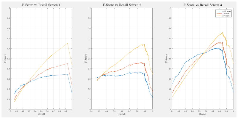
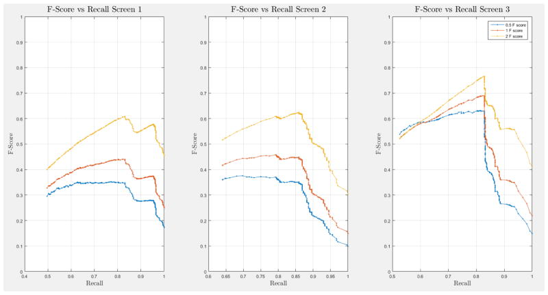
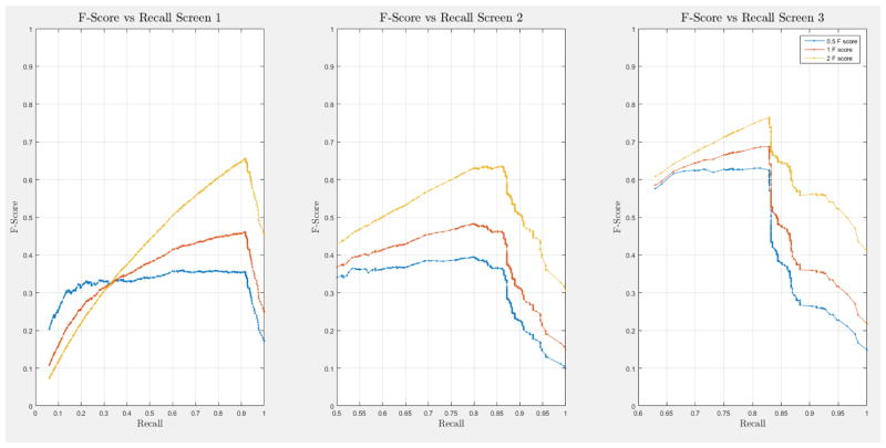
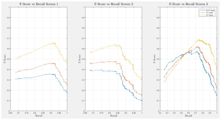
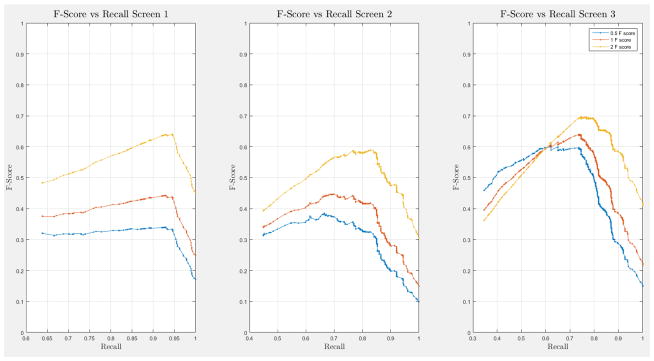
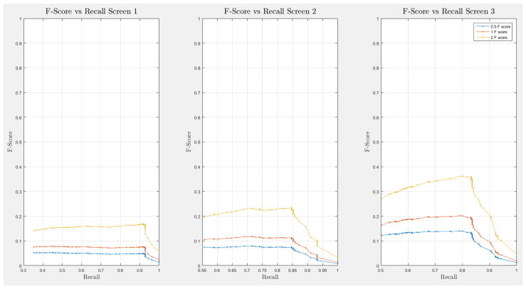
A 10-fold cross-validation was conducted on the complete NLST dataset for each model. The NLST dataset is an imbalanced dataset. The ratio of cancer to non-cancer cases is 1083:24461, or around 1 cancer case for every 24 non-cancer cases. As such, imbalance problems arise in classic cross-validation studies: a model trained mainly from negative cases will tend to be inherently biased towards the majority class. Notably, metrics such as the receiver operating characteristic (ROC) curve and the area under the curve (AUC) can be deceiving when training and testing on imbalanced datasets [42]. In our situation, such an evaluation will always have a high accuracy, and thus would not provide insight into whether the model truly identifies cancer cases and how it compares with other models. More informative metrics for imbalanced datasets include precision, recall, and the F-Score [42]. In Section H, Figure 21 of the Appendix we present the F-score over recall curves of the 10-fold corss-validation evaluation of the Forward-Arrow DBN model with a NoisyMax gate. The F-score curves improve with additional screenings. However, we note here that we cannot truly evaluate whether our model truly identifies cancer cases, compared with other models over the same dataset, given the large number of non-cancer cases that flatten the F-score curves.

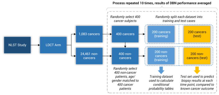
One approach to deal with data imbalance problems is through the use of resampling techniques [43]. In this work, we under-sampled the training and test sets from the majority class (i.e., non-cancer cases) to preserve a 1:1 ratio of the cancer to non-cancer cases. The models were trained and evaluated a total of 10 times. Each time, the training and test sets were randomly selected from the NLST cohort and each consisted of 200 cancer cases and 200 randomly selected non-cancer cases, matched by age and gender. This process was used to assess overfitting and the variability in accuracy of the models, as well as to create a balanced dataset for computing the associated probabilities of a positive Biopsy of an individual. Figure 3 illustrates this process. Additionally, the models were tested against the full NLST dataset to assess generalization.

Figure 3.

The training and testing sets’ random selection process of cases from the NLST dataset. The training and test set consist of 200 cancer and 200 non-cancer cases, respectively. Ten random training and test sets, with replacement, were selected for our analysis.

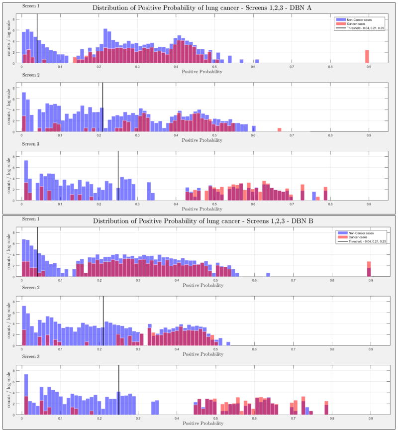
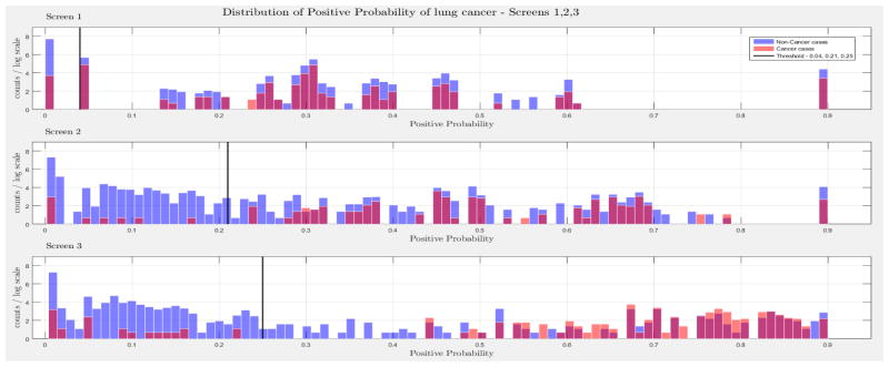
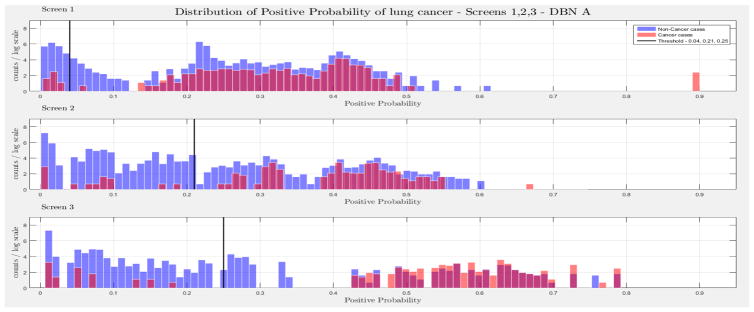
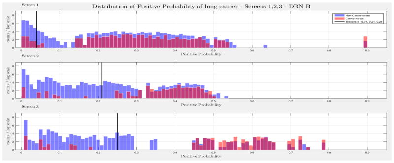
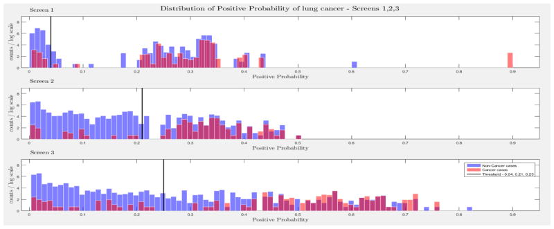
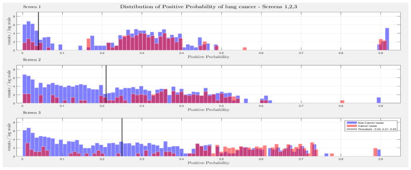
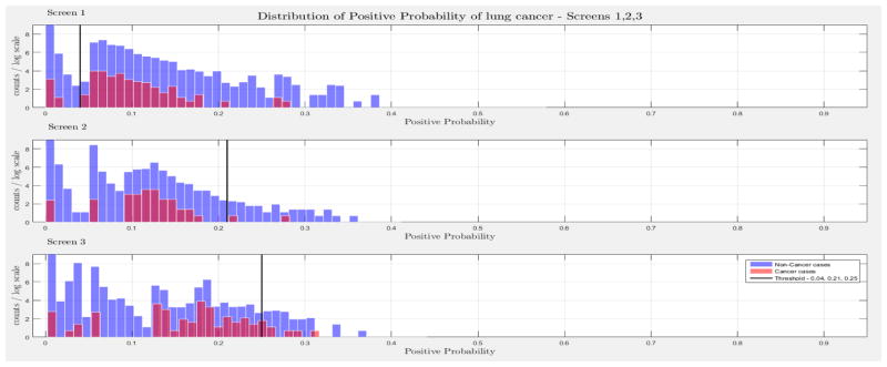
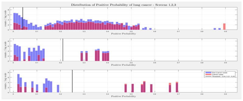
The evaluation of the models was based on the computed probability of the Biopsy variable for a test case, given all prior and current evidence, for each of the three intervention points of the NLST trial. A threshold, θ, was determined for the probability value of Biopsy to indicate a positive biopsy outcome (i.e., probability values below θ were non-cancer cases, values larger or equal to θ were cancer cases). This enabled us to perform a binary classification. A positive case prediction by a physician represents any case that resulted in ordering an additional diagnostic procedure. Subsequently, we present for each screen the sensitivity and counts of cancer cases detected by our models at specific thresholds for θ, which were determined based on the distribution of the positive Biopsy probability values (see Figure 4), as well as the receiver operating characteristic (ROC) curve. For discussion purposes we focus our models’ comparisons with models A and B. Figure 4 depicts the probability of a positive biopsy, as predicted by the models in each screening, of confirmed cancer (red) and non-cancer (blue) cases in the trial. Both DBN A and B tend to discriminate cancer and non-cancer cases better with increasing number of screenings. The thresholds for θ were chosen in a way that favors recall. For example, each threshold aims to minimize the number of cancer cases missed while preserving an acceptable rate of falsely predicted cancer cases. The results for each of the 10 randomization test sets and resultant models as well as the physicians’ predictions were averaged for visualization purposes.

Figure 4.

The combined probability distributions for a positive biopsy, of DBN A (top) and DBN B (bottom), for all cases across the 10 random test sets, for each screen. Red indicates all confirmed cancer cases in the trial, irrespective of screening time points. Blue indicates the confirmed non-cancer cases. The three subplots depict the probability of a positive biopsy in each of the three screening points of the trial. With successive screenings we can see that the probability of a positive biopsy for non-cancer (blue) and cancer (red) cases tends to move towards the left and right side of each subplot, respectively. The solid black lines represent the thresholds chosen to discriminate cancer cases from non-cancer cases in the DBN predictions.

Comparison with experts

Concordance between the models’ positive prediction for a biopsy (i.e., ≥ θ) and a NLST clinician’s recommendation for biopsy and confirmation of lung cancer was determined. The identification of cancer cases was comparable, across the three intervention points of the trial for our lung cancer screening DBNs. In terms of the number of predicted cases and discrimination of the same cases, to physicians’ performance during the NLST, as shown in Table 2. After each screening point, cases that were confirmed as positive lung cancers or deceased were removed in the subsequent screening evaluation. The McNemar’s test for each of the contingency tables of similar cases was significant (p < 0.01), in each of the three intervention points of the trial. This means that the contingency tables of similar cases are asymmetric and confirms that the models minimize the false negative (fn) rate of cancer cases while maintaining an acceptable false positive (fp) rate. Additionally, the 95% C.I. of the type I and II errors (b – c) and of the test of proportions (p₂ – p₁) demonstrate that the direction of this asymmetry is toward the fp cases.

Table 2.

The results of the lung screening DBNs A and B and the Physicians of the NLST Trial for the first, second and third screening, as well as the percentages of equivalent predictions of true positive (tps), false negatives (fns), false positives (fps) and true negatives (tns). Deceased and already identified cancer cases before each intervention point of the trial were excluded from the evaluation of the DBNs as well as the evaluation of the physicians predictions. DBN A and B Predictions: The contingency table that depicts the predictions of the lung screening DBNs for each screening at a threshold of 0.04, 0.21 and 0.25, respectively. Physicians’ Predictions: The contingency table that depicts the predictions of the Physicians in the trial. DBNs A and B and Physicians Concurrence: The percentage of equivalent predictions of tps, fns, fps and tns. For example, the percentage of tps, fns, fps and tns represents how many number of cases where equivalently predicted (i.e., if the same cases are predicted by both the DBN and physicians) as tp, fn, fp and tn by the DBN and the Physicians over the total number of tps, fns, fps and tns, respectively. McNemar’s Test: The chi-square and p-value of the McNemar’s test for the contingency matrix of similar cases identified by the models and the physicians. 95% C.I. (b – c): Confidence Interval of the difference of type I and type II errors of the concordance matrix. 95% C.I. (p₂ – p₁): Confidence Interval of the difference of proportions of the contigency matrix of similar cases.

	DBN A Predictions		DBN B Predictions		Physicians’ Predictions		DBN A & Physicians’ Concurrence		DBN B & Physicians’ Concurrence		McNemar’s Test		95% C.I. (b – c)		95% C.I. (p2 – p1)
											A	B	A	B	A	B
First Screening	53 (tp) 221 (fp)	2 (fn) 121 (tn)	51 (tp) 134 (fp)	4 (fn) 208 (tn)	49 (tp) 108 (fp)	6 (fn) 235 (tn)	70.4% (tp) 49.3% (fp)	35.2% (fn) 46.0% (tn)	71.4% (tp) 59.1% (fp)	48.7% (fn) 73.3% (tn)	x2 = 91.03 p < 1.0 e−10	x2 = 77.39 p < 1.0e−10	b = fp c = fn b – c = 94.5 (77.5,110.57)	b = fp c = fn b – c = 82.1 (64.87,98.69)	$\begin{array}{l}{p}_1=\frac{tp+fn}{N}\\ p_1=\frac{tp+fp}{N}\end{array}$ p2–p1= 0. 3778 (0.3099,0.4421)	$\begin{array}{l}{p}_1=\frac{tp+fn}{N}\\ p_1=\frac{tp+fp}{N}\end{array}$ p2– p1 = 0.2655 (0.2098,0.3192)
Second Screening	27 (tp) 50 (fp)	4 (fn) 244 (tn)	27 (tp) 50 (fp)	4 (fn) 244 (tn)	29 (tp) 61 (fp)	2 (fn) 233 (tn)	69.0% (tp) 39.3% (fp)	30.5% (fn) 78.9% (tn)	68.7% (tp) 39.3% (fp)	29.0% (fn) 79.0% (tn)	x2 = 26.05 p = 3.28e−7	x2 = 25.95 p = 3.5e−7	b = fp c = fn b – c = 28.6 (16.45,39.52)	b = fp c = fn b – c = 28.5 (16.42,39.52)	$\begin{array}{l}{p}_1=\frac{tp+fn}{N}\\ p_1=\frac{tp+fp}{N}\end{array}$ p2–p1 = 0. 1092 (0.0628,0.1509)	$\begin{array}{l}{p}_1=\frac{tp+fn}{N}\\ p_1=\frac{tp+fp}{N}\end{array}$ p2– p1 = 0.1088 (0.0627,0.1509)
Third Screening	35 (tp) 24 (fp)	7 (fn) 227 (tn)	35 (tp) 24 (fp)	7 (fn) 227 (tn)	37 (tp) 32 (fp)	4 (fn) 219 (tn)	71.0% (tp) 41.6% (fp)	46.0% (fn) 85.8% (tn)	71.0% (tp) 41.6% (fp)	46.0% (fn) 85.8% (tn)	x2 = 8.45 p = 0. 0036	x2 = 8.45 p = 0.0036	b = fp c = fn b – c = 12.3 (2.83,21.18)	b = fp c = fn b – c =12.7 (3.61,22.34)	$\begin{array}{l}{p}_1=\frac{tp+fn}{N}\\ p_1=\frac{tp+fp}{N}\end{array}$ p2–p1 = 0. 0492 (0.0113,0.0847)	$\begin{array}{l}{p}_1=\frac{tp+fn}{N}\\ p_1=\frac{tp+fp}{N}\end{array}$ p2– p1 = 0.0507 (0.0144,0.0892)

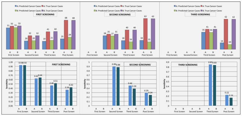
Moreover, we examined whether models A and B can predict the majority of cancer cases at a specific screening point of the NLST trial and assessed whether these models could identify cancer cases before their occurrence. We evaluated how many of our false positive cases in each screening of the trial turned out to be cancer cases later in the trial. Figure 5 illustrates the sensitivity of the lung cancer screening DBNs in each screening, as well as the counts of the predicted number of cancer cases by the models with the total number of true cancer cases in the trial. Figure 5 also illustrates how many false positive cases at a particular screening point of the trial end up being cancer cases in future screening points. Interestingly, a significant portion of false positive cases are cancer cases in subsequent screenings. Note that confirmed cancer cases from the trial first received a LDCT screening exam, and were then subsequently confirmed through the use of additional diagnostic procedures. In comparison, the DBN models infer that these cases are likely cancer without the diagnostic procedure (i.e., the outcome of a biopsy will likely be positive).

Figure 5.

Top: The diagrams represent the true number of cancer cases in each screening point of the trial and the number of cancer cases predicted by the models in each screening. For example, in the leftmost histogram for the first screening, DBN A predicted 51 out of 55 cancer cases. From the same screening we examined the false positive cases and identified how many of those cases were cancer cases in subsequent screenings. In the second screening of the trial there were 32 cancer cases. 20 out of those 32 cancer cases were found to be false positive cases in the first screening of the trial. Similarly, in the third screening, 19 out of 41 cancer cases were false positive cases in the first screening. In the post screening 25 out of 68 cancer cases were false positive cases in the first screening of the trial. The middle diagram represents how many cancer cases were identified in the second screening and how many false positive cancer cases in the second screening are cancer cases in the third and post screening cancer cases. The diagram on the right represents how many cancer cases were identified in the third screening and how many false positive cancer cases in the third screening are cancer cases in the post screening cancer cases. Bottom: (Left) The sensitivity of the lung cancer screening DBNs for the first, second, third, and post-screening cases after the first screening event (baseline). The sensitivities at the second, third, and post-screening cases represent the true positive rate achieved from the pool of false positive cases in the first screen. (Middle) Sensitivity of the DBN for the second, third and post-screening events after the second screening exam. The sensitivities at the third and post-screening cases represent the true positive rate achieved from the pool of false positive cases in the second screen. (Right) The sensitivity of the DBN for the third and post-screening cases after the last screening exam. The sensitivities at the post-screening cases represent the true positive rate achieved from the pool of false positive cases in the third screen.

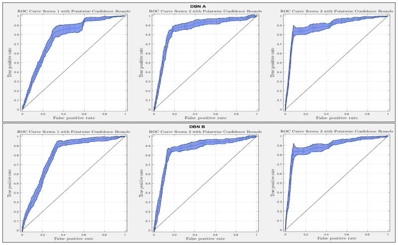
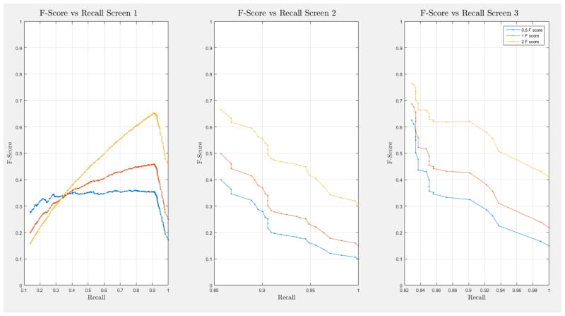
ROC curves with 95% confidence intervals for the first, second, and third screens are shown in Figure 6. Table 3 summarizes the area under the curve (AUC) for each screen’s evaluation and the corresponding confidence interval. The AUC increased with increasing number of screens, which suggests that the models’ predictive power improves with time. The AUCs of the Forward-Arrow DBN without a NoisyMax gate, the two learned DBNs and the naïve Bayes model are similar to DBN A and B and can be found in Table 3. More details on the results of the evaluation of each model are provided in Section F of the Appendix. Overall, all models have similar AUCs and confidence interval (C.I.) of the AUC for each screening. The learned DBNs have similar performance to all models except the AUC and C.I. of the AUC for the first screening of model E, which is lower and higher, respectively, compared with the other models. In addition, as shown by the NLST and the models themselves, performance is improved with consecutive screens. This is evident both from Table 2 as well as the precision/recall (PR) and F-score curves (see Appendix I and H) computed for each screening time point. The desirable performance of PR and F-score curves is to be in the upper-right-hand corner. The PR and F-score curves in Appendix I and H tend to move towards the upper-right-hand corner with increasing number of screenings. Models A-E achieved the best PR curves across screenings with PR curves improving with increasing number of screenings. The worst PR curves, which are in the bottom-left-hand corner, are the naïve Bayes model (see Appendix I). The naïve Bayes PR curves get worse with increasing number of screenings, indicating overfitting to specific features, such as the LDCT outcome. We have also tested the performance of a decision tree on the dataset, using a variation of the C4.5 algorithm. The decision tree performance was extremely low compared to the other models and is not reported.

Figure 6.

The ROC curve of three intervention points of the NLST trial with point-wise 95% confidence bounds.

Table 3.

The AUC and the 95% confidence interval for the first, second and third screening. A: The Forward-Arrow DBN with a NoisyMax gate; B: The Reversed-Arrow DBN; C: The Forward-Arrow DBN without a NoisyMax gate; D: The learned DBN with “compositional” variables; E: The learned DBN without “compositional” variables; F: The naïve Bayes Model.

Model	A		B		C		D		E		F
	AUC	C.I.	AUC	C.I.	AUC	C.I.	AUC	C.I.	AUC	C.I.	AUC	C.I.
First Screening	0.778	0.757 – 0.800	0.798	0.776 – 0.821	0.789	0.774 – 0.804	0.790	0.769 – 0.810	0.751	0.654 – 0.849	0.799	0.777 – 0.821
Second Screening	0.857	0.834 – 0.880	0.858	0.832 – 0.884	0.844	0.819 – 0.869	0.862	0.839 – 0.886	0.853	0.832 – 0.875	0.865	0.844 – 0.885
Third Screening	0.887	0.869 – 0.905	0.887	0.866 – 0.907	0.884	0.863 – 0.906	0.877	0.858 – 0.896	0.878	0.859 – 0.897	0.886	0.866 – 0.907

The models’ predictive power was also assessed by investigating the number of future cancer cases predicted by the models using only observations from one screening. For example, if we were testing for cancer cases at t = 0 (first screening) we assumed that all cancer cases at t > 0 were cancer cases at t = 0 (i.e., ignored time). In this way, we can evaluate how many cancer cases are predicted before incidence. Out of the 121 true positive cases detected by DBN B on the first screening (see Table 6 of the Appendix), given that the DBN predicted 51 cancer cases that were cancer cases of the first screening (see Figure 5 - top left), the DBN predicted 70 additional cancer cases that were diagnosed with cancer later in the trial (see Table 6 in Appendix C).

Assessing model performance given missing data

We grouped all cases in the study that missed the second screen in the NLST, but underwent the first and third screens. There were 417 such cases in the complete NLST dataset, which we used to evaluate whether the models could predict the cancer status (e.g., cancer or non-cancer) of an individual that missed the second LDCT screening exam and was subsequently screened at the third screen. Table 4 provides the contingency tables for these cases that went on to develop cancer by the third screening or after the third screening. DBN A and DBN B managed to predict 8 and 6 out of the 11 cases, respectively, that developed lung cancer by the third screening, and both the DBNs predicted 4 out of 7 cases that developed cancer after the third screening.

Table 4. DBN Predictions By 3^rd Screening.

Contingency table for the individuals that missed the second screen of the trial and by the third screen were diagnosed with cancer at the t = 1 epoch of the DBN. DBN Predictions After 3^rd Screening: Contingency table for the individuals that missed the second screen of the trial and after the third screen were diagnosed with cancer (i.e., third screening cancer).

	DBN A				DBN B
	DBN Predictions By 3rd Screening		DBN Predictions After 3rd Screening		DBN Predictions By 3rd Screening		DBN Predictions After 3rd Screening
Cases that missed the second screening	8 (tp) 91 (fp)	3 (fn) 315 (tn)	4 (tp) 88 (fp)	3 (fn) 311 (tn)	6 (tp) 71 (fp)	5 (fn) 335 (tn)	4 (tp) 67 (fp)	3 (fn) 332 (tn)

The NLST dataset is complete in terms of patient information (i.e, parent nodes). To evaluate the effect of missing data on the parent nodes in the training set and the end performance of the Forward-Arrow DBN without a NoisyMax gate we randomly selected parent nodes and assigned missing data to each one to simulate a “missing at random” scenario. For example, we selected one random parent node and set 50 random cases with missing values for that node. We repeated this in incremental steps of 50 cases up to 350 (our training set consisted of 400 cases). We then reiterated the process with two random parents, increasing up to all parent nodes. Our results showed that the AUC and the confidence interval of the AUC remained relatively stable. Changing the distribution of these priors does not significantly affect performance. The highest impact on performance of the AUC, which was of the order of -0.01, was on the first screening. This subtle change may be attributed to the fact that biopsy and cancer nodes of the first screening are conditionally dependent on the priors. A strength of influence diagram of each structure depicting the influence amongst variables in each network is provided in Appendix E.

Generalization and comparison to other models

We assessed the generalizability/overfitting of the models on the whole NLST dataset. Table 5 depicts that the true positive (tp), false negative (fn), false potive (fp) and true negative (tn) rates of the model over the whole dataset and the random balanced test sets appear stable. The number of test cases in the whole dataset and in the random balanced test set are 25446 and 400, respectively. Lastly, we compared how the full logistic regression model (LR) of [41] without spiculation performs on the NLST cases at baseline. We first evaluated how the LR performs on the NLST cases when trained with NLST cases and we also evaluated how the parameterized model, with parameters published in [41], performs on the NLST cases. In both cases, compared to the DBN, the LR maintains a high true negative rate, a high false negative rate, and a significantly lower true positive rate (see Table 5). The LR models were evaluated only on baseline as they were trained and evaluated in [41].

Table 5.

The true positive (tp), false negative (fn), false potive (fp) and true negative (tn) rates of the DBN and Logistic Regression models. DBN A & B Whole Dataset: The average tp, fn, fp and tn rates of the 10 DBN models trained on 400 cases and evaluated on the remaining NLST dataset of 25, 446 cases. DBN A & B random sets: The average tp, fn, fp and tn rates of the 10 DBN models trained and tested on random balanced sets of 400 cases. Physicians Whole Dataset: The average tp, fn, fp and tn rates of the physicians classifications on the entire NLST dataset of 25, 446 cases. Physicians random sets: The average tp, fn, fp and tn rates of the physicians classifications on the random balanced sets of 400 cases. LR model: The full LR model without spiculation [41] evaluated on 5, 353 cases with nodule information of the NLST at baseline (t = 0). The parameters of the model used in this evaluation were adopted from [41]. LR-trained model: The average tp, fn, fp and tn rates of the logistic regression (LR) model, at baseline (t = 0), trained on 2, 663 cases and tested on 2, 690 cases. Dashes represent the cases for which no tp, fn, fp and tn rates were computed for the LR models.

	First Screening		Second Screening		Third Screening
DBN A, whole dataset	92.6% (tp) 30.2% (fp)	7.40% (fn) 69.8% (tn)	87.3% (tp) 9.40% (fp)	12.7% (fn) 90.6% (tn)	83.9% (tp) 6.70% (fp)	16.1% (fn) 93.3% (tn)
DBN A, random test sets	96.4% (tp) 65.6% (fp)	3.60% (fn) 35.4% (tn)	87.1% (tp) 17.0% (fp)	12.9% (fn) 83.0% (tn)	83.3% (tp) 9.60% (fp)	16.7% (fn) 90.4% (tn)
DBN B, whole dataset	92.6% (tp) 30.2% (fp)	7.40% (fn) 69.8% (tn)	87.3% (tp) 9.40% (fp)	12.7% (fn) 90.6% (tn)	83.9% (tp) 6.9% (fp)	16.1% (fn) 93.1% (tn)
DBN B, random test sets	92.7% (tp) 39.2% (fp)	7.30% (fn) 60.8% (tn)	87.1% (tp) 17.0% (fp)	12.9% (fn) 83.0% (tn)	83.3% (tp) 9.60% (fp)	16.7% (fn) 90.4% (tn)
Physicians, whole dataset	89.7% (tp) 23.2% (fp)	10.3% (fn) 76.8% (tn)	93.7% (tp) 15.0% (fp)	6.30% (fn) 85.0% (tn)	90.1% (tp) 9.60% (fp)	9.90% (fn) 90.4% (tn)
Physicians, random test sets	89.1% (tp) 31.5% (fp)	10.9% (fn) 68.5% (tn)	93.6% (tp) 20.7% (fp)	6.40% (fn) 79.3% (tn)	90.2% (tp) 12.8% (fp)	9.80% (fn) 87.3% (tn)
Logistic Regression [41]	11.0% (tp) 0.50% (fp)	89.0% (fn) 99.5% (tn)	- -	- -	- -	- -
Logistic Regression, retrained	16.3% (tp) 0.8% (fp)	83.7% (fn) 99.2% (tn)	- -	- -	- -	- -

5. Discussion

In this work we built and tested five different DBNs for lung cancer screening prediction using backward construction and structure learning methods. Given the uncertain nature of lung cancer and the necessity to perform a biopsy to confirm the underlying disease we used a three-state cancer state-space model to represent the cancer status of an individual along the screening process. Such a representation offers the following advantages. First, it represents the cancer state of an individual in terms of cancer staging that captures concepts like disease dynamics and nodule growth, instead of the standard binary “yes” and “no” states. Second, the fact that the cancer nodes are never instantiated with evidence due to the uncertainty of the disease during testing (i.e., cancer staging is only validated using additional diagnostic procedures) allows the flow of probabilistic influence of demographic characteristics as well as previous screening outcomes on any screening point of the trial (i.e., via d-separation and sequential configuration). The performance of the learned DBNs is similar to that of the Forward-Arrow and Reversed-Arrow DBNs. The results of the learned structures demonstrate similar relationships to those in the expert-driven Forward-Arrow models with respect to the imaging assessment over time (see Figure 8 in Appendix E); additional relationships were inferred, but without significant change in model performance. Qualitatively, the expert-driven models provide a more straightforward understanding of the relationship between variables over time. Markedly, the NLST trial patient information (e.g., demographics) was captured only at the start of the trial. While some measures are typically invariant over time (e.g., gender), various measures do change over time (e.g., age, body mass index). The underlying dataset did not have these latter variables reflected in subsequent time points in the screening process. In our opinion, it would be inaccurate to model them as such (and the imaging interpretations were also not informed by any such additional information). Nevertheless, given such data at different time points, the performance of the DBNs could improve with additional modeling.

Based on the results of our evaluation, DBN A and B provide results comparable to the radiologists who participated in and read the NLST LDCT imaging studies. We also tested other models on this dataset such as decision trees and a naïve Bayes model, but their performance was suboptimal compared to the DBNs. The use of a DBN for our analysis rather than a BN network as in [32, 33] takes into account the temporal evolution of a cancer, with improved performance in the discriminative ability of the model in future screenings. A standard 10-fold cross-validation method on the entire dataset would be ideal to assess overfitting. But given the class imbalance present in the dataset (1:24 cancer to non-cancer cases), we would not gain insight into the models’ ability for the more important predictive classification of cancer. [43] used similar methods to deal with imbalance in their dataset, but instead chose to oversample the minority class until a 1:1 ratio was achieved in their training set. They also reported metrics such as precision, recall, and F-score to compare performance against imbalanced datasets. The AUC for all networks remained higher than 0.75 in the balanced test sets across the three screening points of the trial, and the AUC curves improve over time. The use of balanced test sets allows the effective comparison of each model in the ROC and PR space over the cancer class. We can see that all models’ performance were comparable in the ROC space (AUC of the ROC). However, in the PR space we also see that all models have a clear advantage over the naïve Bayes model (see Appendix I Figures 23 – 29). This model adjusts to very specific features, such as the LDCT nodes, and thus overfits its predictions on these features. It can accurately discriminate negative cases (comparable AUC to other models); but when asked for the probability of a real cancer case given that this cancer case is predicted by the model (PR curve), its performance is lower.

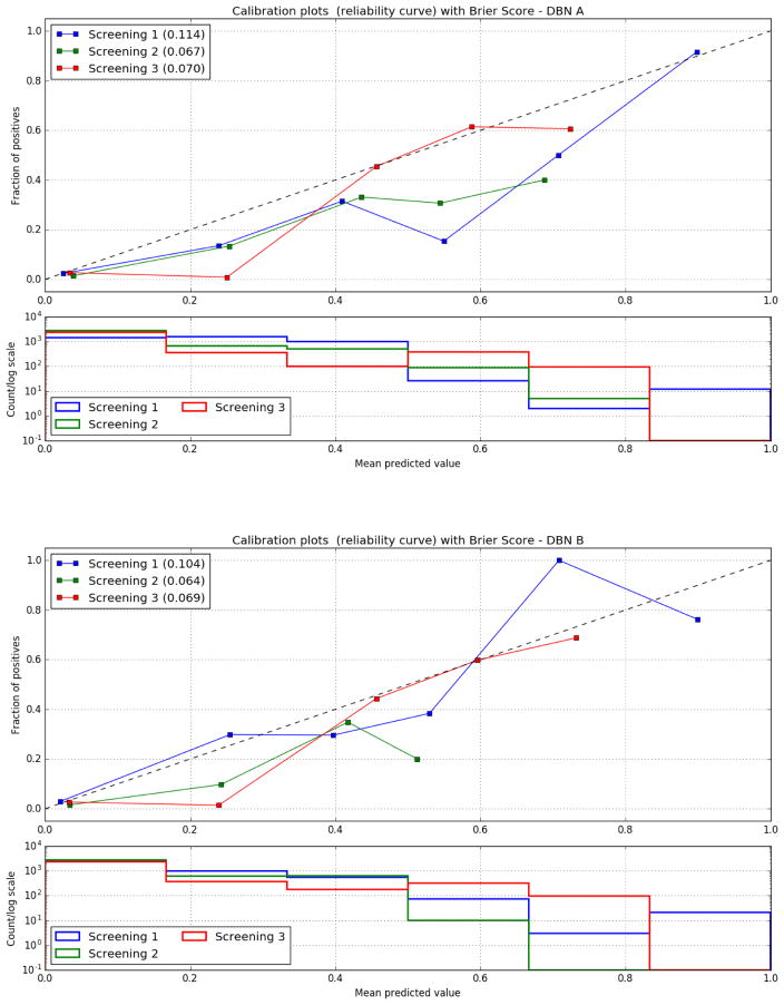
Models A and B were also able to identify a significant number of cases at each intervention point of the trial that were future cancer cases (see Appendix C). The Brier score as well as the calibration curves of DBNs A and B improve with the increasing number of screenings (see Appendix D), demonstrating the ability of the models to perform calibrated cancer incidence predictions over time. Interestingly, the lung screening DBNs A and B only require a small training set, on the order of 50 times smaller than the original dataset, to make predictions on a large number of cases they have never encountered before. The models demonstrate good discrimination when evaluated on the whole NLST dataset. In addition, the tp, fp, fn and tn rates over the whole dataset compared to the random balance test sets are consistent and in some cases better. Still, it is important to note that in this study the DBNs were developed and trained using data from a randomized controlled trial, where information was gathered in structured case report forms and a large degree of standardization took place. Despite the performance over the entire NLST dataset, real-world application of these DBNs will require adaptation to handle observations made from routine clinical screening processes (i.e., adjusting for “noise” and variance). Ultimately, external validation of the DBN is required.

DBNs present certain advantages regarding lung cancer incidence prediction, including their ability to utilize datasets with missing data. Although the NLST dataset is from a controlled trial, and thus is largely complete with only some missing data (e.g., due to individuals missing a screening exam), our models appear to be robust against missing values and still make reasonable predictions in light of missing data. In our investigation of the cancer status of cases that missed only the second NLST screening, both DBN A and B predicted the majority of cases that were cancer cases by the third screening or after the third screening of the trial. Suggesting that certain lung cancer risk factors and the outcome of the first LDCT are sufficient for an accurate future prediction of cancer. This short-term predictive ability may be applicable in cases where missing a screening exam would result in symptomatic cancer. Cases with missing data were also used in the training phase of the DBN without affecting the models’ predictive ability. We can improve the parameterization of a model from cases with incomplete data by only using the information we do have for each case, with incomplete data, for the computation of the corresponding CPT tables of the DBN network. For example, cases that developed lung cancer at the baseline of the trial before they received their first screening exam, even though we do not have information about them after baseline, were still used in the computation of the baseline CPTs (e.g., Gender, Age). To match a real lung cancer screening setting we included all of the aforementioned cases in our evaluation. We used the EM algorithm to train the Forward-Arrow DBN with a NoisyMax gate, the Reversed-Arrow DBN, and both the learned DBNs. One advantage of the EM algorithm is its ability to estimate the parameters of a network using the observed data. In particular, it iteratively fills in missing values with estimated values and subsequently re-estimates the parameters from this complete dataset. We believe it would be inappropriate to estimate the disease status of a deceased individual in subsequent screenings as individuals who died during the course of the trial, or who were diagnosed with cancer, were removed from the screening process of the trial. Thus, in the Forward-Arrow DBN without a NoisyMax gate, we estimated the parameters of this network empirically from observations in the dataset. Interestingly, both techniques provide similar results (see Appendix F). As such, EM would be a more appropriate algorithm in cases that missed a screening exam but is unsuitable with participants who were diagnosed with cancer or who died during the course of the trial. A method that takes into account both types of missing data would be more appropriate in eliminating bias during training. When compared with the full logistic regression model without spiculation [41] the Lung Screening DBNs had better tp, fp and fn rates. This suggests a superior discriminatory power on the NLST dataset. Nevertheless, the LR model’s results in Table 5 are trained and tested on a specific portion of the dataset: individuals with reported nodule abnormalities and nodule consistency. The DBN models, in contrast, were trained on a balanced set of cancer cases and non-cancer cases, with the majority of non-cancer cases without abnormalities. Also, the classification task of each model is somewhat different. For example, our DBN models identify lung cancer individuals whereas the LR model identifies cancerous nodules. Further investigation and standardization of the dataset and the classification task of the different types of models would be more appropriate for such a comparison. But similar to other models, baseline information on smoking status, demographics, health status, history of cancer, and exposure risk factors were employed as inputs. However, we did not use quantitative imaging information. McWilliams et al. [41] utilized the maximum nodule size, the type of nodule, and the number of nodules per CT scan, resulting in a parsimonious multivariate logistic regression model. Their models achieved an AUC higher than 0.90. In this study, we did not explicitly use nodule characteristics in our analysis, but rather included the interpretation of the LDCT by the radiologists, which was based on nodules’ overall growth between consecutive screening exams. We speculate that a nodule’s rate of growth is a significant predictor of lung cancer, as all our models and physicians’ predictions improve given the progression of information. An exploration of how much “history” is needed in terms of interpretation and predictive power is also required: it may be that in this domain, only the past n years of observation are required (rather than the entire longitudinal history). The NLST only provided three time points, so it is not possible to ascertain what amount of information would be optimal for temporal analysis of lung cancer screening data. The use of nodule features such as consistency, location, and size would be strong predictors of lung cancer [44] and will be included in subsequent biterations of our model in combination with automated segmentation methods [45] to automatically provide additional evidence for predicting diagnoses.

We recognize that there are some limitations to this work. For example, the screenings received by the individuals in the NLST were not exactly at the same three discrete time points; (on the contrary they had a continuous nature as individuals received their screenings at different days). Given the nature of real-world implementation of lung screening programs, it is unlikely that a fixed time frequency of observation will occur, for any number of reasons. As such, a DBN may ultimately not be well-suited to handle longer sequences of observation and clinical decision-making. Alternative continuous time temporal models will be explored as part of our future work. Also, the thresholds used in this work were selected to favor recall, providing a conservative prediction that would err on the side of detecting a cancer, rather than missing a cancer case. Thus, the optimal threshold was considered to be one that minimized the number of cancer cases while having an acceptable false positive rate. The use of threshold-determining methods that take into consideration factors such as utility of life and monetary costs will be looked at in the future.

6. Conclusion

In this work we explored five DBNs for lung cancer screening constructed using the results of the NLST study. We demonstrated the challenges in providing screening recommendations using a DBN. We dealt with data imbalance and introduced a training and testing procedure for DBNs in uncertain diseases, such as cancer that uses a hidden cancer node, during testing, built on a cancer staging state-space model. Parameter reduction methods and the EM algorithm for parameterization with missing data were also explored. The DBNs aim to identify individuals who will go on to develop lung cancer based on data collected at baseline and radiologist interpretation in sequential (annual) imaging exams. All models achieved high AUC scores across all three screening points of the NLST, demonstrating comparable performance to the experts. As may be expected, the DBNs performance improved over time, as more information about the history of the patient unfolded. Additionally, the models ability to predict future cancer cases in advance was also examined, finding that they were able to identify some cases before the expert (i.e., cases that were deemed false positives by a radiologist, but that in later studies, proved to be cancer). This work is the first step in understanding how we may subsequently tailor the lung cancer screening process to optimize early detection while minimizing false positive findings.

Appendix

A. Eligibility criteria

The eligibility criteria used to obtain the complete set of 25, 846 cases from the CT arm of the NLST dataset were: 1) the participant to be eligible to participate in the NLST trial in terms of the NLST eligibility criteria (e.g., age between 55–74 years old); 2) the participant’s last contact status to be either active or deceased; and 3) the participant’s case to be neither withdrawn or lost.

B. Variables

Variables used from the NLST data and the associated categories/discretizations in the dynamic Bayesian network are as follows:

Variable Name	Description	Discretization
Age	Age of the individual	Under 60 years old; Between 60 and 70 years old; and More than 70 years old
Gender	Gender of the study subject	Male, female
Smoking status	The smoking status of the individual at the outset of the NLST.	Yes, no
Body mass index (BMI)	Height/weight ratio of the individual at the start of the NLST	Underweight, normal, overweight, obese
Cancer history	Specifies if the individual had a prior history of bladder, breast, cervical, colorectal, esophageal, larynx, lung, nasal, oral, pancreatic, pharynx, stomach, thyroid, or transitional cell cancer.	Yes, no
Disease history	Boolean variable representing the individual’s history of diagnosis of asthma (adult or childhood), COPD, emphysema, fibrosis of the lung, sarcodosis, or tuberculosis.	Yes, no
Work history	Represents work-based exposures related to the development of lung cancer, including asbestos, coal, and other chemicals.	Yes, no
Family history of lung cancer	Boolean variable indicating if an immediate family member (parent, sibling, child) was previously diagnosed with lung cancer.	Yes, no
Cancer	This variable represents the state of the individual to have a suspected lung cancer, based on Figure 1.
LDCT	The outcome of the imaging study for the individual, based on radiologist interpretation.	Screening with abnormalities detected and growth since prior study; Screening with abnormalities detected but no growth or change since prior study; no abnormalities
Biopsy	The results of a diagnostic biopsy.	Positive, negative
Death	Boolean variable giving the probability of death.	Yes, no

C. Prediction of future cancer cases

Table 6.

Top: Contingency table that represents an evaluation of the DBN predictions from the first screen with all cancer cases in the trial in the 10 random balanced test sets, including the cancer cases of the first screening. Middle: a Contingency table that represents an evaluation of the DBN predictions from the second screen with the remaining cancer cases in the trial, including the cancer cases of the second screening. Bottom: A Contingency table that represents an evaluation of the DBN predictions from the third screen with all the remaining cancer cases in the trial, including the cancer cases of the third screening. The 150 true positive cases shown above on the first screening of DBN A, consist of the 51 true positives predicted by the model in the first screening evaluation without taking into consideration the remaining cancer cases of the trial. By including the additional future cancer cases the DBN is able to predict an additional 99 cancer cases which in the initial evaluation were considered as false positives. This means that the majority of false positives predicted in the first screening in future screenings are true cancer cases.

	DBN A Predictions		DBN B Predictions
First Screening	150 (tp) 124 (fp)	47 (fn) 77 (tn)	121 (tp) 64 (fp)	76 (fn) 121 (tn)
Second Screening	58 (tp) 20 (fp)	76 (fn) 172 (tn)	58 (tp) 19 (fp)	76 (fn) 172 (tn)
Third Screening	45 (tp) 13 (fp)	58 (fn) 175 (tn)	45 (tp) 13 (fp)	58 (fn) 175 (tn)

D. Calibration curves

Figure 7.

The calibration curves of the DBN models for each screening as well as the Brier Score. The Brier score decreases with time between screenings. Bottom: Histogram of the positive cases over the probability of a positive Biopsy for each screening.

E. The DBN networks

Figure 8.

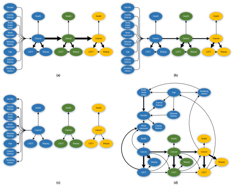
The network Structure and the strength of influence depicted by the arrow thickness connecting the two variables. (a) The Forward-Arrow DBN without the NoisyMax gate; (b) The Forward-Arrow DBN with a NoisyMax gate as a cancer node at t = 0; (c) The Reversed-Arrow DBN; (d) The Learned Network with compositional nodes. The Learned DBN without compositional variables is not depicted due to the high complexity in structure.

Table 7.

Structure learning algorithm parameters.

Structure Learning
Dataset number of cases	25046
Learning Algorithm	Bayesian Search
Algorithm Parameters
Max parent count	8
Iterations	20
Sample size	50
Seed	0
Link Probability	0.1
Prior Link Probability	0.001
Background Knowledge
Forced Arcs	5
Nodes assigned to tiers	6

F. Statistics

We present the results of the performance of each DBN structure over the same random balanced test sets of 400 cases (200 cancer and 200 non-cancer cases). All DBNs were trained on balanced training sets of 400 cases (200 cancer and 200 non-cancer cases). The thresholds used in these evaluations are 0.04, 0.21 and 0.25 for each screening, respectively.

F.1. The Forward-Arrow DBN without a NoisyMax gate

The Forward-Arrow DBN without a NoisyMax Gate was not parameterized using the EM algorithm. All nodes CPT tables’ probabilities were empirically estimated from the dataset observations except from the Biopsy (abstracted from literature) and Death (death rate at baseline) nodes which were fixed nodes and the Cancer node at baseline. The Cancer variable would be impossible to parameterize without imposing some domain assumptions about an individual’s cancer state as this node consists of 2304 parameters and 3 states (Non-cancer, In Situ, Invasive Cancer). The data do not contain sufficient observations to represent every single parameter (i.e., combination of parent state to effect node state). We dealt with this parameterization problem by using the following two assumptions. First, we assumed that every state combination with no instances in the In Situ or Invasive Cancer state in our data would imply that the majority of instances are in the Non-cancer state. Second, when we had data instances for either the Situ or Invasive-cancer state, we computed the probabilities of those states and assumed that the remaining cases were in the Non-cancer states (i.e., probability complement). The reason we pursued this parameterization approach is that most existing training algorithms do not support the use of missing data (e.g., dead patients with no observations in subsequent screenings). For example, EM would be a more appropriate algorithm in the case of missing values (i.e., missing value of age or BMI). In such a case an EM algorithm would instead estimate a statistical estimate of that value. We believe it would be undesirable to estimate the disease status of a deceased individual in subsequent screenings as deceased/diagnosed with cancer individuals were removed from the screening process of the trial.

Table 8.

The tp, fp, tn, fn rates and the counts of tp, fp, tn, fn of the DBN for each screen respectively. The thresholds used for each screening were 0.04, 0.21 and 0.25 for screen 1,2 and 3 respectively.

The Forward-Arrow DBN without a NoisyMax gate
	Screen 1		Screen 2		Screen 3
Rates	0.927 (tp) 0.347 (fp)	0.073 (fn) 0.653 (tn)	0.903 (tp) 0.228 (fp)	0.097 (fn) 0.772 (tn)	0.854 (tp) 0.139 (fp)	0.146 (fn) 0.861 (tn)
Counts	51 (tp) 119 (fp)	4 (fn) 224 (tn)	28 (tp) 67 (fp)	3 (fn) 227 (tn)	35 (tp) 35 (fp)	6 (fn) 216 (tn)

Table 9.

The reported AUCs of the ROC and the C.I. of the AUCs for each screening.

	AUCs	AUCs C.I.	Interval
First Screening	0.789	0.774 – 0.804	0.0304
Second Screening	0.844	0.819 – 0.869	0.0496
Third Screening	0.884	0.863 – 0.906	0.0435

F.2. The Forward-Arrow DBN with a NoisyMax gate

Table 10.

The tp, fp, tn, fn rates and the counts of tp, fp, tn, fn of the DBN for each screen respectively. The thresholds used for each screening were 0.04, 0.21 and 0.25 for screen 1,2 and 3 respectively.

The Forward-Arrow DBN with a NoisyMax gate
	Screen 1		Screen 2		Screen 3
Rates	0.96 (tp) 0.65 (fp)	0.04 (fn) 0.35 (tn)	0.87 (tp) 0.17 (fp)	0.13 (fn) 0.83 (tn)	0.83 (tp) 0.10 (fp)	0.17 (fn) 0.90 (tn)
Counts	53 (tp) 221 (fp)	2 (fn) 121 (tn)	27 (tp) 50 (fp)	4 (fn) 244 (tn)	35 (tp) 24 (fp)	7 (fn) 227 (tn)

Table 11.

The reported AUCs of the ROC and the C.I. of the AUCs for each screening.

	AUCs	AUCs C.I.	Interval
First Screening	0.778	0.757 – 0.800	0.043
Second Screening	0.857	0.834 – 0.880	0.046
Third Screening	0.887	0.869 – 0.905	0.035

F.3. Reversed-Arrow DBN

Table 12.

The tp, fp, tn, fn rates and the counts of tp, fp, tn, fn of the DBN for each screen respectively. The thresholds used for each screening were 0.04, 0.21 and 0.25 for screen 1,2 and 3 respectively.

Reversed-Arrow DBN
	Screen 1		Screen 2		Screen 3
Rates	0.93 (tp) 0.39 (fp)	0.07 (fn) 0.61 (tn)	0.87 (tp) 0.17 (fp)	0.13 (fn) 0.83 (tn)	0.83 (tp) 0.10 (fp)	0.17 (fn) 0.90 (tn)
Counts	51 (tp) 134 (fp)	4 (fn) 208 (tn)	27 (tp) 50 (fp)	4 (fn) 244 (tn)	34 (tp) 24 (fp)	7 (fn) 227 (tn)

Table 13.

The reported AUCs of the ROC and the C.I. of the AUCs for each screening.

	AUCs	AUCs C.I.	Interval
First Screening	0.798	0.776 – 0.821	0.045
Second Screening	0.858	0.832 – 0.884	0.052
Third Screening	0.887	0.866 – 0.907	0.041

F.4. Learned DBN with compositional variables (structure learning)

Table 14.

The tp, fp, tn, fn rates and the counts of tp, fp, tn, fn of the DBN for each screen respectively. The thresholds used for each screening were 0.04, 0.21 and 0.25 for screen 1,2 and 3 respectively. Bottom:

Learned DBN with compositional variables
	Screen 1		Screen 2		Screen 3
Rates	0.93 (tp) 0.36 (fp)	0.07 (fn) 0.64 (tn)	0.87 (tp) 0.18 (fp)	0.13 (fn) 0.82 (tn)	0.81 (tp) 0.10 (fp)	0.19 (fn) 0.90 (tn)
Counts	51 (tp) 122 (fp)	4 (fn) 220 (tn)	27 (tp) 53 (fp)	4 (fn) 241 (tn)	34 (tp) 26 (fp)	8 (fn) 225 (tn)

Table 15.

The reported AUCs of the ROC and the C.I. of the AUCs for each screening.

	AUCs	AUCs C.I.	Interval
First Screening	0.790	0.769 – 0.810	0.040
Second Screening	0.862	0.839 – 0.886	0.047
Third Screening	0.877	0.858 – 0.896	0.038

F.5. Learned DBN without compositional variables

Table 16.

The tp, fp, tn, fn rates and the counts of tp, fp, tn, fn of the DBN for each screen respectively. The thresholds used for each screening were 0.04, 0.21 and 0.25 for screen 1,2 and 3 respectively.

Learned DBN without compositional variables
	Screen 1		Screen 2		Screen 3
Rates	0.95 (tp) 0.42 (fp)	0.05 (fn) 0.58 (tn)	0.81 (tp) 0.17 (fp)	0.19 (fn) 0.83 (tn)	0.83 (tp) 0.11 (fp)	0.17 (fn) 0.89 (tn)
Counts	52 (tp) 145 (fp)	3 (fn) 198 (tn)	26 (tp) 51 (fp)	6 (fn) 244 (tn)	34 (tp) 28 (fp)	7 (fn) 222 (tn)

Table 17.

The reported AUCs of the ROC and the C.I. of the AUCs for each screening.

	AUCs	AUCs C.I.	Interval
First Screening	0.751	0.654 – 0.849	0.195
Second Screening	0.853	0.832 – 0.875	0.043
Third Screening	0.878	0.859 – 0.897	0.038

F.6. Naïve Bayes (NB)

Table 18.

Top: The tp, fp, tn, fn rates and the counts of tp, fp, tn, fn of the DBN for each screen respectively. The thresholds used for each screening were 0.04, 0.21 and 0.25 for screen 1,2 and 3 respectively. Bottom:

Naïve Bayes
	Screen 1		Screen 2		Screen 3
Rates	0.927 (tp) 0.392 (fp)	0.073 (fn) 0.608 (tn)	0.871 (tp) 0.170 (fp)	0.129 (fn) 0.830 (tn)	0.833 (tp) 0.096 (fp)	0.167 (fn) 0.904 (tn)
Counts	51 (tp) 134 (fp)	4 (fn) 208 (tn)	27 (tp) 50 (fp)	4 (fn) 244 (tn)	35 (tp) 24 (fp)	7 (fn) 227 (tn)

Table 19.

The reported AUCs of the ROC and the C.I. of the AUCs for each screening.

	AUCs	AUCs C.I.	Interval
First Screening	0.799	0.777 – 0.821	0.044
Second Screening	0.865	0.844 – 0.885	0.041
Third Screening	0.886	0.866 – 0.907	0.041

G. The Probability Distributions over each screen of confirmed cancer and Non-cancer cases

G.1. The Forward-Arrow DBN without a NoisyMax gate

Figure 9.

The combined probability distributions for a positive biopsy for all cases across the 10 random test sets, for each screen. Red indicates all confirmed cancer cases in the trial, irrespective of time. Blue indicates the confirmed non-cancer cases. The 3 subplots depict the probability of a positive biopsy in each of the three screening points of the trial. With successive screenings we can see that the probability of a positive biopsy for non-cancer (blue) and cancer (red) cases tends to move towards the left and right side of each subplot, respectively. The solid black lines represent the thresholds chosen to discriminate cancer cases from non-cancer cases in the DBN predictions.

G.2. The Forward-Arrow DBN with a NoisyMax gate

Figure 10.

The combined probability distributions for a positive biopsy for all cases across the 10 random test sets, for each screen. Red indicates all confirmed cancer cases in the trial, irrespective of time. Blue indicates the confirmed non-cancer cases. The 3 subplots depict the probability of a positive biopsy in each of the three screening points of the trial. With successive screenings we can see that the probability of a positive biopsy for non-cancer (blue) and cancer (red) cases tends to move towards the left and right side of each subplot, respectively. The solid black lines represent the thresholds chosen to discriminate cancer cases from non-cancer cases in the DBN predictions.

G.3. Reversed-Arrow DBN

Figure 11.

The combined probability distributions for a positive biopsy for all cases across the 10 random test sets, for each screen. Red indicates all confirmed cancer cases in the trial, irrespective of time. Blue indicates the confirmed non-cancer cases. The 3 subplots depict the probability of a positive biopsy in each of the three screening points of the trial. With successive screenings we can see that the probability of a positive biopsy for non-cancer (blue) and cancer (red) cases tends to move towards the left and right side of each subplot, respectively. The solid black lines represent the thresholds chosen to discriminate cancer cases from non-cancer cases in the DBN predictions.

G.4. Learned DBN with compositional variables

Figure 12.

The combined probability distributions for a positive biopsy for all cases across the 10 random test sets, for each screen. Red indicates all confirmed cancer cases in the trial, irrespective of time. Blue indicates the confirmed non-cancer cases. The 3 subplots depict the probability of a positive biopsy in each of the three screening points of the trial. With successive screenings we can see that the probability of a positive biopsy for non-cancer (blue) and cancer (red) cases tends to move towards the left and right side of each subplot, respectively. The solid black lines represent the thresholds chosen to discriminate cancer cases from non-cancer cases in the DBN predictions.

G.5. Learned DBN without compositional variables

Figure 13.

The combined probability distributions for a positive biopsy for all cases across the 10 random test sets, for each screen. Red indicates all confirmed cancer cases in the trial, irrespective of time. Blue indicates the confirmed non-cancer cases. The 3 subplots depict the probability of a positive biopsy in each of the three screening points of the trial. With successive screenings we can see that the probability of a positive biopsy for non-cancer (blue) and cancer (red) cases tends to move towards the left and right side of each subplot, respectively. The solid black lines represent the thresholds chosen to discriminate cancer cases from non-cancer cases in the DBN predictions.

G.6. 10-fold cross validation of the Forward-Arrow DBN with a NoisyMax gate

Figure 14.

The combined probability distributions for a positive biopsy for all cases across the 10 random test sets, for each screen. Red indicates all confirmed cancer cases in the trial, irrespective of time. Blue indicates the confirmed non-cancer cases. The 3 subplots depict the probability of a positive biopsy in each of the three screening points of the trial. With successive screenings we can see that the probability of a positive biopsy for non-cancer (blue) and cancer (red) cases tends to move towards the left and right side of each subplot, respectively. The solid black lines represent the thresholds chosen to discriminate cancer cases from non-cancer cases in the DBN predictions.

G.7. Naïve Bayes

Figure 15.

The combined probability distributions for a positive biopsy for all cases across the 10 random test sets, for each screen. Red indicates all confirmed cancer cases in the trial, irrespective of time. Blue indicates the confirmed non-cancer cases. The 3 subplots depict the probability of a positive biopsy in each of the three screening points of the trial. With successive screenings we can see that the probability of a positive biopsy for non-cancer (blue) and cancer (red) cases tends to move towards the left and right side of each subplot, respectively. The solid black lines represent the thresholds chosen to discriminate cancer cases from non-cancer cases in the DBN predictions.

H. F-Scrore curves

H.1. The Forward-Arrow DBN without a NoisyMax gate

Figure 16.

F-score over recall curve.

H.2. The Forward-Arrow DBN with a NoisyMax gate

Figure 17.

F-score over recall curve.

H.3. Reversed-Arrow DBN

Figure 18.

F-score over recall curve.

H.4. Learned DBN with compositional variables

Figure 19.

F-score over recall curve.

H.5. Learned DBN without compositional variables

Figure 20.

F-score over recall curve.

H.6. 10-fold cross validation of the Forward-Arrow DBN with a NoisyMax gate

Figure 21.

F-score over recall curve.

H.7. Naïve Bayes (NB)

Figure 22.

F-score over recall curve.

I. PR Curves of the original model

I.1. The Forward-Arrow DBN without a NoisyMax gate

Figure 23.

The precision and recall curve.

I.2. The Forward-Arrow DBN with a NoisyMax gate

Figure 24.

The precision and recall curve.

I.3. Reversed-Arrow DBN

Figure 25.

The precision and recall curve.

I.4. Learned DBN with compositional variables

Figure 26.

The precision and recall curve.

I.5. Learned DBN without compositional variables

Figure 27.

The precision and recall curve.

I.6. 10-fold cross validation of the Forward-Arrow DBN with a NoisyMax gate

Figure 28.

The precision and recall curve.

I.7. Naïve Bayes (NB)

Figure 29.

The precision and recall curve.

J. Missing values statistics

Table 20.

Parent Nodes Missing value counts.

		Age	BMI	Family History	Disease History	Cancer History	Smoking Status	Work Exposure	Gender
Count	Present values	25846	25573	25846	25846	25846	25846	25846	25846
	Missing values	0	93	0	0	0	0	0	0
Fraction	Present values	1	0.9964	1	1	1	1	1	1
	Missing values	0	0.0036	0	0	0	0	0

Table 21.

LDCT nodes outcomes missing values. The missing values of these nodes consist of individuals that died, were diagnosed with cancer and are administered treatment and individuals that missed a screening exam.

		LDCT Screen 1 Outcome	LDCT Screen 2 Outcome	LDCT Screen 3 Outcome
Count	Present values	25827	24335	23696
	Missing values	19	1511	2150
Fraction	Present values	0.9993	0.942	0.917
	Missing values	0.0007	0.058	0.083

References

- 1.Siegel R, Naishadham D, Jemal A. Cancer statistics, 2013. CA: a cancer journal for clinicians. 2013;63(1):11–30. doi: 10.3322/caac.21166. [DOI] [PubMed] [Google Scholar]
- 2.Siegel RL, Miller KD, Jemal A. Cancer statistics, 2015. CA: a cancer journal for clinicians. 2015;65(1):5–29. doi: 10.3322/caac.21254. [DOI] [PubMed] [Google Scholar]
- 3.American Cancer Society. Cancer Facts & Figures 2015. 2015:1–9. http://www.cancer.org/acs/groups/content/@editorial/documents/document/acspc-044552.pdf.
- 4.Bach PB, Mirkin JN, Oliver TK, Azzoli CG, Berry DA, Brawley OW, et al. Benefits and Harms of CT Screening for Lung Cancer. Jama. 2012;307(22):2418–2429. doi: 10.1001/jama.2012.5521. /pmc/articles/PMC3709596/?report=abstract. [DOI] [PMC free article] [PubMed] [Google Scholar]
- 5.Watson W, Conte A. Lung cancer and smoking. The American Journal of Surgery. 1955;89(2):447–456. doi: 10.1016/0002-9610(55)90087-8. [DOI] [PubMed] [Google Scholar]
- 6. [accessed: 2015-7-28];Cancer statistics for the UK. 2015 May 13; http://www.cancerresearchuk.org/health-professional/cancer-statistics.
- 7.Howlander N, Noone A, Krapcho M, Garshell J, Miller D, Altekruse S, et al. Seer cancer statistics review, 1975–2011. national cancer institute; bethesda, md: 2013. 2014. [Google Scholar]
- 8.NLSTR Team. Aberle DR, Adams AM, Berg CD, Black WC, Clapp JD, et al. Reduced lung-cancer mortality with low-dose computed tomographic screening. The New England journal of medicine. 2011;365(5):395–409. doi: 10.1056/NEJMoa1102873. http://dx.doi.org/10.1056/NEJMoa1102873. [DOI] [PMC free article] [PubMed] [Google Scholar]
- 9.Patz EF, Pinsky P, Gatsonis C, Sicks JD, Kramer BS, Tammemägi MC, et al. Overdiagnosis in low-dose computed tomography screening for lung cancer. JAMA internal medicine. 2014;174(2):269–274. doi: 10.1001/jamainternmed.2013.12738. http://dx.doi.org/10.1001/jamainternmed.2013.12738. [DOI] [PMC free article] [PubMed] [Google Scholar]
- 10.Bourzac K. Diagnosis: Early warning system. Nature. 2014;513(7517):S4–S6. doi: 10.1038/513s4a. http://dx.doi.org/10.1038/513s4a. [DOI] [PubMed] [Google Scholar]
- 11.Maisonneuve P, Bagnardi V, Bellomi M, Spaggiari L, Pelosi G, Rampinelli C, et al. Lung cancer risk prediction to select smokers for screening CT a model based on the italian COSMOS trial. Cancer Prevention Research. 2011;4(11):1778–1789. doi: 10.1158/1940-6207.CAPR-11-0026. http://dx.doi.org/10.1158/1940-6207.CAPR-11-0026. [DOI] [PubMed] [Google Scholar]
- 12.Bach PB, Kattan MW, Thornquist MD, Kris MG, Tate RC, Barnett MJ, et al. Variations in lung cancer risk among smokers. Journal of the National Cancer Institute. 2003;95(6):470–478. doi: 10.1093/jnci/95.6.470. http://dx.doi.org/10.1093/jnci/95.6.470. [DOI] [PubMed] [Google Scholar]
- 13.Gail MH, Costantino JP, Bryant J, Croyle R, Freedman L, Helzlsouer K, et al. Weighing the risks and benefits of tamoxifen treatment for preventing breast cancer. Journal of the National Cancer Institute. 1999;91(21):1829–1846. doi: 10.1093/jnci/91.21.1829. http://www.ncbi.nlm.nih.gov/pubmed/10547390. [DOI] [PubMed] [Google Scholar]
- 14.Freedman AN, Seminara D, Gail MH, Hartge P, Colditz GA, Ballard-Barbash R, et al. Cancer risk prediction models: a workshop on development, evaluation, and application. J Natl Cancer Inst. 2005;97(10):715–723. doi: 10.1093/jnci/dji128. [DOI] [PubMed] [Google Scholar]
- 15.Etzel CJ, Bach PB. Estimating individual risk for lung cancer. Seminars in Respiratory and Critical Care Medicine. 2011;32(1):3–9. doi: 10.1055/s-0031-1272864. https://www.thieme-connect.com/products/ejournals/html/10.1055/s-0031-1272864. [DOI] [PubMed] [Google Scholar]
- 16.Cronin KA, Gail MH, Zou Z, Bach PB, Virtamo J, Albanes D. Validation of a model of lung cancer risk prediction among smokers. Journal of the National Cancer Institute. 2006;98(9):637–640. doi: 10.1093/jnci/djj163. http://www.ncbi.nlm.nih.gov/pubmed/16670389. [DOI] [PubMed] [Google Scholar]
- 17.Raji OY, Duffy SW, Agbaje OF, Baker SG, Christiani DC, Cassidy A, et al. Predictive accuracy of the liverpool lung project risk model for stratifying patients for computed tomography screening for lung cancer: a case-control and cohort validation study. Annals of internal medicine. 2012;157(4):242–250. doi: 10.7326/0003-4819-157-4-201208210-00004. http://dx.doi.org/10.7326/0003-4819-157-4-201208210-00004. [DOI] [PMC free article] [PubMed] [Google Scholar]
- 18.Spitz MR, Hong W, Amos CI, Wu X, Schabath MB, Dong Q, et al. A risk model for prediction of lung cancer. Journal of the National Cancer Institute. 2007;99(9):715–726. doi: 10.1093/jnci/djk153. http://dx.doi.org/10.1093/jnci/djk153. [DOI] [PubMed] [Google Scholar]
- 19.Spitz MR, Etzel CJ, Dong Q, Amos CI, Wei Q, Wu X, et al. An expanded risk prediction model for lung cancer. Cancer Prevention Research. 2008;1(4):250–254. doi: 10.1158/1940-6207.CAPR-08-0060. http://dx.doi.org/10.1158/1940-6207.CAPR-08-0060. [DOI] [PMC free article] [PubMed] [Google Scholar]
- 20.Tammemagi MC, Pinsky PF, Caporaso NE, Kvale PA, Hocking WG, Church TR, et al. Lung cancer risk prediction: Prostate, lung, colorectal and ovarian cancer screening trial models and validation. Journal of the national cancer institute. 2011;103(13):1058–1068. doi: 10.1093/jnci/djr173. http://dx.doi.org/10.1093/jnci/djr173. [DOI] [PMC free article] [PubMed] [Google Scholar]
- 21.Ltifi H, Trabelsi G, Ayed M, Alimi A. Dynamic Decision Support System Based on Bayesian Networks Application to fight against the Nosocomial Infections. (IJARAI) International Journal of Advanced Research in Artificial Intelligence. 2012;1(1):22–29. http://arxiv.org/abs/1211.2126. [Google Scholar]
- 22.Charitos T, van der Gaag LC, Visscher S, Schurink KA, Lucas PJ. A dynamic Bayesian network for diagnosing ventilator-associated pneumonia in ICU patients. Expert Systems with Applications. 2009;36(2):1249–1258. doi: 10.1016/j.eswa.2007.11.065. http://www.sciencedirect.com/science/article/pii/S0957417407005805. [DOI] [Google Scholar]
- 23.Verduijn M, Rosseel PMJ, Peek N, de Jonge E, de Mol BAJM. Prognostic Bayesian networks. II: An application in the domain of cardiac surgery. Journal of Biomedical Informatics. 2007;40(6):619–630. doi: 10.1016/j.jbi.2007.07.004. [DOI] [PubMed] [Google Scholar]
- 24.Cuaya G, Muñoz-Meléndez A, Carrera LN, Morales EF, Quiñones I, Pérez AI, et al. A dynamic Bayesian network for estimating the risk of falls from real gait data. Medical and Biological Engineering and Computing. 2013;51(1–2):29–37. doi: 10.1007/s11517-012-0960-2. http://link.springer.com/10.1007/s11517-012-0960-2. [DOI] [PubMed] [Google Scholar]
- 25.Watt EW, Bui AAT. Evaluation of a dynamic bayesian belief network to predict osteoarthritic knee pain using data from the osteoarthritis initiative. AMIA 2008 Symposium; 2008. pp. 788–92. http://www.pubmedcentral.nih.gov/articlerender.fcgi?artid=2656041{&}tool=pmcentrez{&}rendertype=abstract. [PMC free article] [PubMed] [Google Scholar]
- 26.Pardalos PM, Xanthopoulos P, Zervakis M, Exarchos KP, Rigas G, Goletsis Y, et al. Modelling of Oral Cancer Progression Using Dynamic Bayesian Networks. Vol. 25. Springer US; 2012. http://link.springer.com/10.1007/978-1-4614-2107-8{_}11. [DOI] [Google Scholar]
- 27.Stojadinovic A, Bilchik A, Smith D, Eberhardt JS, Ward EB, Nissan A, et al. Clinical decision support and individualized prediction of survival in colon cancer: Bayesian belief network model. Annals of Surgical Oncology. 2012;20(1):161–174. doi: 10.1245/s10434-012-2555-4. http://dx.doi.org/10.1245/s10434-012-2555-4. [DOI] [PubMed] [Google Scholar]
- 28.Austin RM, Onisko A. Increased cervical cancer risk associated with extended screening intervals after negative human papillomavirus test results : Bayesian risk estimates using the Pittsburgh Cervical Cancer Screening Model. Journal of the American Society of Cytopathy. 2015;1(1):9–14. doi: 10.1016/j.jasc.2015.05.001. http://dx.doi.org/10.1016/j.jasc.2015.05.001. [DOI] [PubMed] [Google Scholar]
- 29.Cruz-Ramírez N, Acosta-Mesa HG, Carrillo-Calvet H, Alonso Nava-Fernández L, Barrientos-Martínez RE. Diagnosis of breast cancer using Bayesian networks: A case study. Computers in Biology and Medicine. 2007;37(11):1553–1564. doi: 10.1016/j.compbiomed.2007.02.003. arXiv:arXiv:1401.0852v2. [DOI] [PubMed] [Google Scholar]
- 30.Velikova M, Lucas P. A decision support system for breast cancer detection in screening programs. Ecai. 2008;178:658–662. doi: 10.3233/978-1-58603-891-5-658. http://ebooks.iospress.nl/Download/Pdf/4454. [DOI] [Google Scholar]
- 31.Maskery SM, Hu H, Hooke J, Shriver CD, Liebman MN. A bayesian derived network of breast pathology co-occurrence. Journal of Biomedical Informatics. 2008;41(2):242–250. doi: 10.1016/j.jbi.2007.12.005. http://dx.doi.org/10.1016/j.jbi.2007.12.005. [DOI] [PubMed] [Google Scholar]
- 32.Gevaert O, Smet FD, Timmerman D, Moreau Y, Moor BD. Predicting the prognosis of breast cancer by integrating clinical and microarray data with bayesian networks. Bioinformatics. 2006;22(14):e184–e190. doi: 10.1093/bioinformatics/btl230. http://dx.doi.org/10.1093/bioinformatics/btl230. [DOI] [PubMed] [Google Scholar]
- 33.Oh JH, Craft J, Lozi RA, Vaidya M, Meng Y, Deasy JO, et al. A bayesian network approach for modeling local failure in lung cancer. Physics in Medicine and Biology. 2011;56(6):1635–1651. doi: 10.1088/0031-9155/56/6/008. http://dx.doi.org/10.1088/0031-9155/56/6/008. [DOI] [PMC free article] [PubMed] [Google Scholar]
- 34. [accessed: 2016-7-11];American Joint Committee on Cancer, Lung Cancer Staging. 2009 https://cancerstaging.org/references-tools/quickreferences/Documents/LungCancerStagingPosterUpdated.pdf.
- 35.Koller D, Friedman N. Probabilistic graphical models: principles and techniques. MIT press; 2009. [Google Scholar]
- 36.Van Gerven MA, Taal BG, Lucas PJ. Dynamic bayesian networks as prognostic models for clinical patient management. Journal of biomedical informatics. 2008;41(4):515–529. doi: 10.1016/j.jbi.2008.01.006. http://dx.doi.org/10.1016/j.jbi.2008.01.006. [DOI] [PubMed] [Google Scholar]
- 37.Druzdzel MJ. SMILE : Structural Modeling, Inference, and Learning Engine and GeNIe: A Development Environment for Graphical Decision-Theoretic Models. Proceedings of the Sixteenth National Conference on Artificial Intelligence (AAAI-99) 1999;99:342–343. http://www.pitt.edu/{~}druzdzel/psfiles/aaai99.pdf. [Google Scholar]
- 38.Uusitalo L. Advantages and challenges of Bayesian networks in environmental modelling. Ecological Modelling. 2007;203(3):312–318. doi: 10.1016/j.ecolmodel.2006.11.033. [DOI] [Google Scholar]
- 39.Kraaijeveld P, Druzdzel MJ. GeNIeRate: An interactive generator of diagnostic Bayesian network models. Proc 16th Int Workshop on Principles of Diagnosis. 2005:175–180. doi:10.1.1.102.5119. http://citeseerx.ist.psu.edu/viewdoc/download?doi=10.1.1.102.5119{&}rep=rep1{&}type=pdf.
- 40.Poe RH, Tobin RE. Sensitivity and specificity of needle biopsy in lung malignancy. American Review of Respiratory Disease. 1980;122(5):725–729. doi: 10.1164/arrd.1980.122.5.725. http://www.atsjournals.org/doi/10.1164/arrd.1980.122.5.725. [DOI] [PubMed] [Google Scholar]
- 41.McWilliams A, Tammemagi MC, Mayo JR, Roberts H, Liu G, Soghrati K, et al. Probability of cancer in pulmonary nodules detected on first screening CT. The New England journal of medicine. 2013;369(10):910–919. doi: 10.1056/NEJMoa1214726. http://www.pubmedcentral.nih.gov/articlerender.fcgi?artid=3951177{&}tool=pmcentrez{&}rendertype=abstract. [DOI] [PMC free article] [PubMed] [Google Scholar]
- 42.He H, Garcia EA. Learning from imbalanced data. IEEE Transactions on Knowledge and Data Engineering. 2009;21(9):1263–1284. doi: 10.1109/TKDE.2008.239. http://dx.doi.org/10.1109/TKDE.2008.239. [DOI] [Google Scholar]
- 43.Orphanou K, Stassopoulou A, Keravnou E. DBN-extended: A Dynamic Bayesian network model extended with temporal abstractions for coronary heart disease prognosis. IEEE journal of biomedical and health informatics. 2015;20(3):944–952. doi: 10.1109/JBHI.2015.2420534. http://ieeexplore.ieee.org/lpdocs/epic03/wrapper.htm?arnumber=7080845. [DOI] [PubMed] [Google Scholar]
- 44.van’t Westeinde SC, de Koning HJ, Xu DM, Hoogsteden HC, van Klaveren RJ. How to deal with incidentally detected pulmonary nodules less than 10 mm in size on CT in a healthy person. Lung Cancer. 2008;60(2):151–159. doi: 10.1016/j.lungcan.2008.01.020. http://www.ncbi.nlm.nih.gov/pubmed/18359124. [DOI] [PubMed] [Google Scholar]
- 45.Shen S, Bui AAT, Cong J, Hsu W. An automated lung segmentation approach using bidirectional chain codes to improve nodule detection accuracy. Computers in Biology and Medicine. 2015;57:139–149. doi: 10.1016/j.compbiomed.2014.12.008. http://www.ncbi.nlm.nih.gov/pubmed/25557199. [DOI] [PMC free article] [PubMed] [Google Scholar]