Superensemble forecasts of dengue outbreaks

Abstract

In recent years, a number of systems capable of predicting future infectious disease incidence have been developed. As more of these systems are operationalized, it is important that the forecasts generated by these different approaches be formally reconciled so that individual forecast error and bias are reduced. Here we present a first example of such multi-system, or superensemble, forecast. We develop three distinct systems for predicting dengue, which are applied retrospectively to forecast outbreak characteristics in San Juan, Puerto Rico. We then use Bayesian averaging methods to combine the predictions from these systems and create superensemble forecasts. We demonstrate that on average, the superensemble approach produces more accurate forecasts than those made from any of the individual forecasting systems.

1. Introduction

Recent work has demonstrated that accurate forecasts of the timing and severity of infectious disease outbreaks can be generated using a framework combining a dynamical model of disease transmission and data-assimilation methods [1–5]. However, because no model perfectly represents transmission dynamics in the real world, infectious disease forecasts made by a single model are prone to error due to this model misspecification. In weather and climate forecasting, this problem has been addressed by combining forecasts from multiple competing models in a superensemble. The intent is that some of the biases inherent in the different models will offset so that the superensemble produces more accurate predictions than those generated by any individual model. Such improvement has indeed been observed [6–8].

Dengue is a viral mosquito-borne disease that has spread rapidly over the past 50 years, and is currently endemic in over 100 countries [9]. There are an estimated 360 million dengue infections per year, approximately 25% of which lead to apparent symptoms ranging from mild fever to life threatening haemorrhagic fever and shock [10]. In Puerto Rico, dengue virus was first isolated in 1963, and all four virus serotypes have been circulating on the island since 1982 [11]. As in the rest of the Americas [12], dengue incidence in Puerto Rico has been increasing over the past two decades, with major outbreaks occurring in 1994, 1998, 2007 and 2010 [11]. The annual cost of dengue illness in Puerto Rico has been estimated at $38.7 million, or $10.40 per person [13].

While there is no specific treatment for dengue, simple fluid replacement and case management can reduce the fatality rate for severe dengue from 20% to less than 1% [14]. However, during major dengue outbreaks, hospitals may lack the capacity to administer this basic treatment, leading to preventable deaths. It is, therefore, of great value for public health officials and healthcare facilities to have advance warning of increased dengue cases.

Dengue forecasts and early warning systems have been proposed using a number of approaches, including autoregressive integrative moving average (ARIMA) models [15,16], regression models [17–19], a spatio-temporal hierarchical Bayesian model [20], a percentile rank model [21] and an empirical Bayes model [21]. Other approaches have been used to forecast influenza, including stochastic agent-based models [22,23] and meta-population models [24]. These forecasting systems use various environmental, epidemiological and demographic predictors to generate estimates of future disease incidence.

Here, we develop three distinct forecasting systems for dengue outbreaks in San Juan, Puerto Rico, and then use Bayesian averaging methods to combine the predictions from these systems and create superensemble forecasts. We demonstrate that on average, this approach leads to more accurate forecasts than those made from any of the individual forecasting approaches.

2. Material and methods

2.1. Data

Weekly dengue incidence data from April 1990 through April 2013 for the San Juan-Carolina-Caguas Metropolitan Statistical Area in Puerto Rico were provided by the Puerto Rico Department of Health and Centers for Disease Control and Prevention. These data were collected by the Passive Dengue Surveillance System for dengue case reporting. Dengue cases were generally laboratory confirmed, with the exception of periods of high transmission when suspected cases exceeded laboratory testing capacity, or when case information was incomplete. During these events, additional positive cases from specimens that were not tested were estimated by multiplying the number of untested specimens by the fraction of tested specimens that were laboratory positive [11].

2.2. Forecasting targets

Dengue in Puerto Rico follows a roughly seasonal cycle, generally peaking in the late autumn or early winter months. Dengue seasons are defined as calendar week 17 (late April) through calendar week 16 of the following year. We produced forecasts of three characteristics for each dengue outbreak season: the maximum number of cases reported in a single week (peak incidence), the week during which peak incidence occurs (peak timing) and the total number of cases in the season (total incidence).

2.3. Forecast systems

Three distinct systems were used to produce competing retrospective forecasts of peak timing, peak incidence and total incidence. We call these: F1_N for forecasts generated using a model-inference framework, F2_N for forecasts generated using a Bayesian weighting of historical outbreaks and F3_N for forecasts derived from historical likelihood functions (see below). Forecasts were generated every week, w, for each outbreak season, N, during the ‘testing period’, defined as seasons 15 (year 2005/2006) through 23 (year 2012/2013). Training forecasts TF1, TF2 and TF3 were produced using the F1, F2 and F3 forecast methods, respectively, over the ‘training period’, prior seasons 1 through N − 1, and used to determine the contribution of each individual forecast to the weighted sum superensemble forecasts.

2.3.1. Forecast method 1: susceptible–infectious–recovered-ensemble adjustment Kalman filter

F1 forecasts were produced using a model of disease transmission in conjunction with the ensemble adjustment Kalman filter (EAKF) data-assimilation method, as described in detail in Shaman & Karspeck [1]. The disease transmission model was a basic susceptible–infectious–recovered (SIR) compartmental model [25], commonly used for infectious disease simulation. The model assumes a perfectly mixed population and is governed by the following equations:

2.1

;and

2.2

;where N is the population size (arbitrarily 100 000 people), S and I are, respectively, the number of susceptible and infectious individuals in the population, D is the mean duration of infection and β is the contact rate. The basic reproductive number, R₀, is related to the contact rate by R₀ = βD. For model scaling, we assumed the number of dengue cases observed in clinics represented 20% of total new infections each week.

This model is a greatly simplified representation of dengue transmission. Many processes, including infection rates within the mosquito population and interactions between dengue serotypes, are not explicitly modelled. Previous studies have used such simple compartmental models of human populations to gain insight into dengue transmission dynamics [26,27]. We chose this parsimonious model structure because we lacked data on mosquito infection rates and information on the immunological history of individual cases (e.g. whether an observed case is a primary or secondary infection). Such data would be necessary to constrain a more complex model of disease transmission for generation of reliable forecasts.

The SIR model was used in conjunction with an EAKF. The EAKF consists of an ensemble of SIR model replicates, in this study 400, initialized from a randomly drawn suite of state variable conditions and parameter values, and iteratively optimized over the course of an outbreak in a prediction-update cycle. In the prediction step, the SIR model moves each ensemble member forward until the next observation becomes available, which in this study occurred weekly. In the update step, the EAKF algorithm (see Anderson [28] for full algorithm details) assimilates new observations by adjusting the ensemble members such that their mean and variance match the posterior mean and variance predicted by Bayes' rule.

In addition to running the ensemble SIR-EAKF system forward in time and producing weekly posterior updates, we also used those posteriors to generate weekly forecasts. That is, following each new assimilation of an observation, the updated ensemble of model simulations was propagated forward using the latest parameter and state variable estimates to produce an ensemble forecast of disease incidence through the remainder of the season. Forecasts of the outbreak characteristics (peak timing, peak incidence and total incidence) were derived from the forecast trajectory of the ensemble mean.

Multiplicative inflation was included in the simulation to avoid filter divergence, which can occur in part due to differences between the simplified SIR model structure and true infection dynamics [1]. Here we assumed the dengue incidence data have normally distributed error with variance σ² = 65.

Initial conditions for state variables and parameter values of each ensemble member were randomly selected from the following probability distributions functions: D ∼ Uniform [2 days, 10 days], R₀ ∼ Uniform [1,4], S(t = 0) ∼ Uniform [0,0.6 × N] and I(t = 0) ∼ Exponential [mean = 40].

2.3.2. Forecast method 2: Bayesian weighted outbreaks

The second forecasting method employs a statistical approach in which the current outbreak as observed thus far is described as a weighted average of outbreak trajectories from prior seasons. Similar approaches have been used previously to forecast influenza [29,30] and dengue [21]. Here, the respective weights for each candidate trajectory were determined using Bayesian model averaging (BMA), a statistical method that is commonly used to combine information from competing models [31–33], and was adapted by Raftery et al. [34] for use with dynamic weather forecasts.

The candidate trajectories used to construct forecasts of the outbreak in season N were the preceding seasons, 1 through N − 1, smoothed by applying a five-week centred moving average. More specifically, weeks t − 4 through t of the current season N are estimated as a weighted sum of weekly incidence during weeks t − 4 through t from prior seasons 1 through N − 1. A forecast is then generated by projecting that weighted sum for weeks t + 1 until the end of the season, week 52. The weightings of prior season incidence data are obtained using the probability distribution function (PDF)

2.3

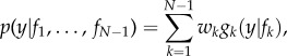
;where y is the weekly dengue incidence, f_k is a candidate outbreak trajectory, w_k is the probability of trajectory f_k being the best representation for season N, and g_k(y|f_k) is the PDF of y conditional on f_k, given that f_k is the best candidate model.

The conditional PDF for y given each candidate trajectory is assumed to be normally distributed with mean f_k and standard deviation σ. For simplicity, we assume equal σ for all candidate trajectories. We use maximum-likelihood estimation over the training window of 5 weeks to obtain w_k and σ (see Raftery et al. [34] for full details). The weights, which sum to 1, are then applied to the candidate trajectories to produce the weighted sum forecast.

2.4

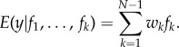
;The resulting trajectory of predicted weekly dengue incidence is used to predict peak timing, peak incidence and total incidence.

2.3.3. Forecast method 3: historical likelihood

Historical likelihood forecasts, F3_N, are made by fitting probability distribution functions to historical data for each of the target outbreak characteristics, observed for seasons 1 through N − 1. Peak timing is described by a normal distribution, while peak incidence and total incidence are described by gamma distributions. As the dengue season progresses and possible outcomes are eliminated, the probability distributions are updated, as described in the electronic supplementary material, Supplementary Methods. The resulting forecast is the expected value of each variable, calculated using the updated PDFs.

2.4. Creating the superensemble

Given a number of competing forecasts, we can produce a superensemble forecast by using a weighted average of the individual forecasts. Using the same BMA technique used to create the weighted analogue forecast, we combine first two (F1 and F2), (F1 and F3), (F2 and F3) and then three (F1, F2 and F3) competing forecasts to produced superensemble forecasts SE(F1,F2), SE(F1,F3), SE(F2,F3) and SE(F1,F2,F3), respectively.

Weights among the three individual forecasting methods were based on the performance of those forecasts over prior seasons (1 through N − 1). For example to produce the superensemble forecast for season 15, we used the training forecasts TF1, TF2, TF3 (described below) for seasons 1 through 14. For season 16, we repeat the process and produce a new set of historical forecasts for seasons 1 through 15, incorporating the additional information from season 15. Note that for the superensemble, BMA is applied across seasons to weight the forecast performance of each method, whereas in F2 it is used to weight how well prior season observations match the present season as thus far observed.

The forecasts for TF1_N, which are acquired independently for each season, only required evaluation of the performance over the prior N − 1 seasons using the same methodology as described for the F1_N forecasts. Methods F2_N and F3_N use prior observations to produce a forecast for season N, and this pool of observations enlarges with each additional season. To evaluate the F2_N forecast accuracy, given the availability of N − 1 seasons, a leave-one-out (LOO) approach was used to construct TF2_N forecasts for each of those N − 1 prior seasons. For example, the set of TF2 forecasts used to inform superensemble weightings for season 15 is the set of 14 LOO forecasts for seasons 1 through 14. Each LOO forecast is the weighted average of the remaining 13 smoothed trajectories. A similar approach was used for the TF3_N forecasts.

In using BMA to combine the individual F1, F2 and F3 forecasts into a superensemble forecast, we find the weights of the three competing forecasting systems for each outbreak characteristic over the training period seasons 1:N − 1, pooled over all forecast weeks 1:52. Equation (2.3) becomes

2.5

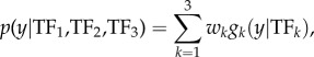
;where y is the target outbreak characteristic, w_k is the probability that forecast method k is the most accurate method and g_k(y|TF_k) is the PDF of y, conditional on TF_k, given that TF_k is the most accurate forecast. This conditional PDF is assumed to be normal with mean TF_k and standard deviation σ. For simplicity, we assume equal σ for all candidate trajectories. We use maximum-likelihood estimation over the entire set of training forecasts to obtain w_k and σ (see again Raftery et al. [34] for full details).

The weights, which sum to 1, are then applied to the three candidate forecasts to produce the weighted sum superensemble forecast. Equation (2.4) becomes

2.6

;For comparison, we produced a final set of forecasts by taking an equal-weighted average of the competing individual forecasts.

2.5. Forecast evaluation

The accuracy of each forecast was evaluated by the absolute error of the prediction relative to observation. We ranked the accuracy of the individual forecasts, simple averages and superensembles by comparing mean absolute error (MAE) aggregated over all seasons and forecast periods, as well as stratified by the week of forecast generation and forecast lead time.

3. Results

Weekly individual forecasts for each season of the initial training period, seasons 1–14, are shown in figures 1–3. Forecast results during the testing period are shown grouped by the week each forecast was produced (figure 4), and by lead time with respect to the outbreak peak, defined as the difference in weeks between when the forecast was generated and the actual or predicted outbreak peak (electronic supplementary material, Supplementary Results, figures S1–S2).

Figure 1.

Weekly TF1 (blue), TF2 (red) and TF3 (yellow) forecasts of peak timing for years 1 through 14. The horizontal black line indicates the true timing of the outbreak peak. The dotted black line also shows the timing of the observed peak; forecasts to the left of this line were made prior to the peak and forecasts to the right were made after the true peak had passed.

Figure 2.

Weekly TF1 (blue), TF2 (red) and TF3 (yellow) forecasts of peak incidence for years 1 through 14. The horizontal black line indicates the true peak incidence. The dotted black line shows the timing of the observed peak; forecasts to the left of this line were made prior to the peak and forecasts to the right were made after the true peak had passed.

Figure 3.

Weekly TF1 (blue), TF2 (red) and TF3 (yellow) forecasts of total incidence for years 1 through 14. The horizontal black line indicates the true total incidence. The dotted black line shows the timing of the observed peak; forecasts to the left of this line were made prior to the peak and forecasts to the right were made after the true peak had passed.

Figure 4.

Mean absolute error by week of forecast over the 9-year testing period. F1, F2 and F3 forecast absolute errors are shown in blue, red and yellow, respectively. Mean absolute error for SE(F1,F2) and SE(F1,F2,F3) superensemble forecasts are in purple and green, respectively.

Different inaccuracies are identifiable for each of the individual forecast approaches. The F1 forecasts frequently predicted false, overly small peaks early in the season when only a few dengue cases had been observed; however, later in the season, during the growth phase of the outbreak, larger outbreaks were forecast, which in some cases overestimated the true size of the outbreak (for example, figures 1–3, seasons 2 and 8). The forecasts improved still later in the season as more observations were assimilated. The F1 forecasts were especially skilled at detecting when the actual peak had passed, leading to high accuracy in peak timing and peak incidence after the true peak (figures 1 and 2).

The F2 forecasts use a weighted sum of historical outbreaks. These forecasts are, therefore, constrained to the range of observed trajectories, but are able to adapt to observational data throughout the dengue season by adjusting the weights assigned to each contributing historical outbreak. While this forecasting system frequently produced better forecasts than F1 and F3, it was subject to large errors, particularly during years when observations followed an unfamiliar trajectory, such as season 3, which had unusually high numbers of observed dengue cases during the first few weeks of the season despite ultimately concluding as a relatively small outbreak. Of the three individual forecasts of peak week, F2 had the lowest MAE on average (figure 4). Like the F1 forecasts, F2 forecasts quickly detected the true peak, leading to accurate estimates of peak timing and peak incidence once the true peak had passed (figures 1 and 2).

F3 forecasts are based on long-term averages of outbreak characteristics; as a result, they did well when such characteristics were close to mean conditions (for example, figures 1 and 2, season 8; figure 3, season 3). In addition, the F3 forecasts were not prone to large error; the largest errors in these forecasts were smaller than those of F1 and F2 (figures 1–3). This is an important advantage, as grossly inaccurate forecasts can have serious public health impacts. However, because this forecasting system possesses limited ability to adapt its forecasts in response to observations, it was slow to arrive at the true value for outbreaks that did not resemble the long-term average (figure 1, season 9; figures 2 and 3, season 13).

The MAE and maximum error of all forecasts made over the testing period (seasons 15–23) are shown for each individual forecast in table 1. p-Values reported here and in electronic supplementary material, table S1, indicate significant MAE differences among pairs of forecast approaches. Overall, F2 produced better forecasts of peak timing than F1 and F3 (p < 0.0001), which had similar MAE. F1 and F2 had equivalent MAE for peak and total incidence during the testing period, and both outperformed F3 (p < 0.016). As in the training forecasts, the maximum errors in F3 forecasts were substantially smaller than those of F1 and F2 for all three outbreak characteristics (table 1).

Table 1.

Mean absolute error over all forecasts.

	forecast mean absolute error			forecast maximum absolute error
	peak timing (weeks)	peak incidence (cases)	total incidence (cases)	peak timing (weeks)	peak incidence (cases)	total incidence (cases)
individual forecasts
F1	4.8	25	519	37.0	399	4565
F2	3.4	23	522	27.0	262	4711
F3	4.5	34	615	21.9	141	3418
superensemble forecasts
SE(F1,F2)	3.3	21	473	27.0	174	3764
SE(F1,F3)	4.3	23	507	22.4	225	3987
SE(F2,F3)	3.8	21	505	24.5	214	3774
SE(F1,F2,F3)	3.7	20	486	24.6	159	3678

The contribution of F1_N, F2_N and F3_N to the weighted sum superensemble forecasts was determined based on the performance of training forecasts TF1, TF2 and TF3 (figures 1–3) during seasons 1 through N − 1 (i.e. the training period). The weights assigned to each forecast are shown in figure 5. In general, the F2 and F3 forecasts were weighted more heavily than F1 for superensemble forecasts of peak timing, while F1 and F2 dominated superensemble forecasts of peak incidence, and to a lesser extent, total incidence. The change in weights over time indicates the lack of consensus on the relative skill of each individual forecast. Each successive year incorporates an additional year of training forecasts and observations, giving a more informed estimate of the average performance of each individual forecasting system.

Figure 5.

Contributions of the F1 (blue), F2 (red) and F3 (yellow) individual forecasts to the weighted sum superensemble forecasts for each season during the testing period (season 15–23). The left column shows weights for forecasts of peak timing, the middle column shows weights for forecasts of peak incidence and the right column shows weights for forecasts of total incidence. The top three rows show the weights for superensemble forecasts using combinations of two individual forecasts, and the bottom row shows weights for superensemble forecasts using all three individual forecasts.

On average, SE(F1,F2) performed better at predicting peak timing than any of the individual forecasts (p < 0.023, table 1). Superensemble forecasts of peak timing that included F3 had a MAE greater than that of F2, but lower than F1 and F3 (p < 0.018). The outbreak peaks were closer to the long-term mean during the training period (mean difference 3.2 weeks) than during the testing period (mean difference 6.9 weeks). As a result, the F3 forecast, which is based on the long-term mean, performed well during the training period and was assigned a relatively high weight in the superensemble, but had larger errors during the testing period, which were passed on to the superensemble forecasts. The superensemble weights adjusted over time to discount the F3 forecast (figure 5). All superensemble forecasts of peak and total incidence had MAE equal to or lower than any individual forecast. Superensemble forecasts all had maximum errors greater than the maximum error in F3, but less than or equal to the maximum errors of F1 and F2 (table 1).

Among the superensemble forecasts using only two individual forecasts, SE(F1,F2) consistently had MAE lower than or equal to SE(F2,F3) and SE(F1,F3) (figure 4) and forecast lead time (electronic supplementary material, figures S1–S2). SE(F1,F2) was heavily weighted towards F2 for predictions of peak timing, and therefore had similar MAE to this forecast (figure 4). In contrast with forecasts of peak timing, where the superensemble forecasts were only as good as the best individual forecast, superensemble forecasts of peak incidence outperformed all three individual forecasts for several weeks in the early season, indicating that the biases of the individual forecasts were offset (figure 4). The superensemble forecasts did not provide a consistent advantage for predicted total incidence; both superensemble forecasts had greater MAE than one or more individual forecasts for most weeks; however, on average over all weeks the superensemble forecasts had lower MAE than the individual forecasts (table 1).

We tested the sensitivity of our results to the parameters and initial conditions of the individual forecast methods and found that the superensemble approach consistently provides greater forecast accuracy compared with the individual forecasts being averaged (electronic supplementary material, Supplemental Results, figure S3, table S2).

4. Discussion

Here we have presented three distinct systems for forecasting dengue incidence, each with certain strengths and weaknesses. By combining these individual forecasts, superensemble forecasts were generated that offset some individual system biases, while retaining reliable aspects of each forecast. Superensemble forecasts of peak and total incidence generally had MAE equal to or lower than any individual forecast. The superensemble forecasts also had lower maximum error than the F1 and F2 individual forecasts.

The findings here serve as a proof-of-concept for infectious disease forecast. The improved accuracy of the superensemble forecasts may have been somewhat limited by the relatively small number of outbreaks available for model training. For example, superensemble forecasts of peak timing were negatively affected by the relatively poor performance of F3 during the testing period, compared with the training period when the weights were assigned. The superensemble weights adjusted as more seasons were added to the training period, decreasing the contribution of the F3 system. We expect that the methods presented here will provide an even larger advantage for diseases, such as influenza, for which more observational data are available to inform superensemble weights.

We also expect the superensemble performance will improve further when more individual forecasting systems are used and the weightings among these candidate systems deviate more strongly from a simple average [35]. Indeed, the SE(F1,F2) and SE(F1,F2,F3) forecasts presented here performed only marginally better than a straight average (i.e. equal weighting) of individual forecasts, with the superensemble providing the greatest advantages over the straight ensemble in cases when the weights assigned to the respective forecasting systems are furthest from equal weighting (electronic supplementary material, table S3).

The methods presented here can incorporate any number and any type of competing forecasts. For example, the F1 forecast presented here used a very simplified model of disease transmission. Additional data on mosquito density and infection rates, as well as improved information on human immunology and dengue serotype interactions could be used to fit more realistic mechanistic models of dengue transmission, which could then be included in the superensemble. Similarly, we could include forecasts using stochastic models that simulate the infectious state of discrete individuals within a population while accounting for demographic noise [23,36]. The superensemble approach provides a formal method to weigh the strengths and limitations of each distinct forecast approach.

Additional training data are also expected to lead to greater advantages in using the weighted superensemble forecasts over the simple average forecasts. In this study, we used a constant weight for each season's forecasts, as the amount of data was not sufficient to justify further stratification of superensemble weighting. However, the relative strength of each forecast method varied based on circumstances such as the timing of the forecast (both with respect to the calendar week, and relative to the predicted outbreak peak, figures 1–4; electronic supplementary material, figures S1–S2), as well as indicators contained within the individual forecasts and in the observed data. For example, F1 forecasts have large errors early in the season but do well near and after the outbreak peak. Forecast indicators that can be used to inform superensemble weights for these F1 forecasts might include within-ensemble variance of the model-inference system and forecast streak (the number of consecutive forecasts predicting the same result), both of which have been previously shown to predict forecast accuracy [2,37]. The number of observed dengue cases in the weeks preceding a forecast relative to observations during those weeks in previous seasons might also be used to indicate whether the weighting of the historically based F2 and F3 forecasts are appropriate; for example F1 forecasts function well during a larger than usual outbreak, whereas the F2 and F3 forecasts might be prone to error and could, therefore, be discounted. If observations are available for multiple locations, as in the case of influenza, the relative performance of competing forecasts might be varied based on geographical and demographic characteristics [2]. Given sufficient data, the derivation of superensemble weights can be binned, or stratified, by metrics such as these in order to produce more specific weights.

5. Conclusion

In summary, we have demonstrated the use of a superensemble approach in order to combine information from multiple competing forecasts of disease incidence. As more real-time forecasts of infectious disease outbreaks are operationalized and incorporated into public health decision-making, it will be increasingly important to reconcile disparate forecasts and combine information from each in order to obtain the most accurate prediction of an unfolding disease outbreak. The work presented here is a first example of such a process.

Data accessibility

The data used to produce forecasts are available at http://dengueforecasting.noaa.gov/.

Authors' contributions

T.K.Y. and J.S. conceived and designed the experiments; T.K.Y. and S.K. performed the experiments; T.K.Y. and J.S. analysed the results; T.K.Y. and J.S. wrote the paper. All authors gave final approval for publication.

Competing interests

J.S. declares partial ownership in S.K. Analytics. T.K.Y. and S.K. declare no competing interests.

Funding

This work was supported by US NIH grant no. GM100467 (J.S.) and GM110748 (T.K.Y., S.K., J.S.), as well as NIEHS Center grant ES009089 (J.S.) and the Defense Threat Reduction Agency contract HDTRA1-15-C-0018 (T.K.Y., J.S.).

References

- 1.Shaman J, Karspeck A. 2012. Forecasting seasonal outbreaks of influenza. Proc. Natl Acad. Sci. USA 109, 20 425–20 430. ( 10.1073/pnas.1208772109) [DOI] [PMC free article] [PubMed] [Google Scholar]
- 2.Shaman J, Karspeck A, Yang W, Tamerius J, Lipsitch M. 2013. Real-time influenza forecasts during the 2012–2013 season. Nat. Commun. 4, 2837 ( 10.1038/ncomms3837) [DOI] [PMC free article] [PubMed] [Google Scholar]
- 3.Yang W, Karspeck A, Shaman J. 2014. Comparison of filtering methods for the modeling and retrospective forecasting of influenza epidemics. PLoS Comput. Biol. 10, e1003583 ( 10.1371/journal.pcbi.1003583) [DOI] [PMC free article] [PubMed] [Google Scholar]
- 4.Dukic V, Lopes HF, Polson NG. 2012. Tracking epidemics with Google flu trends data and a state-space SEIR model. J. Am. Stat. Assoc. 107, 1410–1426. ( 10.1080/01621459.2012.713876) [DOI] [PMC free article] [PubMed] [Google Scholar]
- 5.Ong JBS, Chen M, Cook AR, Lee HC, Lee VJ, Lin RTP, Tambyah PA, Goh LG. 2010. Real-time epidemic monitoring and forecasting of H1N1-2009 using influenza-like illness from general practice and family doctor clinics in Singapore. PLoS ONE 5, e10036 ( 10.1371/journal.pone.0010036) [DOI] [PMC free article] [PubMed] [Google Scholar]
- 6.Krishnamurti TN, et al. 2001. Real-time multianalysis-multimodel superensemble forecasts of precipitation using TRMM and SSM/I products. Mon. Weather Rev. 129, 2861–2883. ( 10.1175/1520-0493(2001)129%3C2861:RTMMSF%3E2.0.CO;2) [DOI] [Google Scholar]
- 7.Yun W, Stefanova L, Krishnamurti T. 2003. Improvement of the multimodel superensemble technique for seasonal forecasts. J. Clim. 16, 3834–3840. ( 10.1175/1520-0442(2003)016%3C3834:IOTMST%3E2.0.CO;2) [DOI] [Google Scholar]
- 8.Krishnamurti TN, Kishtawal CM, LaRow TE, Bachiochi DR, Zhang Z, Williford CE, Gadgil S, Surendran S. 1999. Improved weather and seasonal climate forecasts from multimodel superensemble. Science 285, 1548–1550. ( 10.1126/science.285.5433.1548) [DOI] [PubMed] [Google Scholar]
- 9.Guzman MG. 2015. A new moment for facing dengue? Pathog. Glob. Health 109, 2–3. ( 10.1179/2047772415Z.000000000247) [DOI] [PMC free article] [PubMed] [Google Scholar]
- 10.Bhatt S, et al. 2013. The global distribution and burden of dengue. Nature 496, 504–507. ( 10.1038/nature12060) [DOI] [PMC free article] [PubMed] [Google Scholar]
- 11.Sharp TM, et al. 2013. Virus-specific differences in rates of disease during the 2010 dengue epidemic in Puerto Rico. PLoS Negl. Trop. Dis. 7, e2159 ( 10.1371/journal.pntd.0002159) [DOI] [PMC free article] [PubMed] [Google Scholar]
- 12.Brathwaite Dick O, San Martín JL, Montoya RH, del Diego J, Zambrano B, Dayan GH. 2012. The history of dengue outbreaks in the Americas. Am. J. Trop. Med. Hyg. 87, 584–593. ( 10.4269/ajtmh.2012.11-0770) [DOI] [PMC free article] [PubMed] [Google Scholar]
- 13.Halasa YA, Shepard DS, Zeng W. 2012. Economic cost of dengue in Puerto Rico. Am. J. Trop. Med. Hyg. 86, 745–752. ( 10.4269/ajtmh.2012.11-0784) [DOI] [PMC free article] [PubMed] [Google Scholar]
- 14.Guzman MG, Harris E. 2015. Dengue. Lancet 385, 453–465. ( 10.1016/S0140-6736(14)60572-9) [DOI] [PubMed] [Google Scholar]
- 15.Silawan T, Singhasivanon P, Kaewkungwal J, Nimmanitya S, Suwonkerd W. 2008. Temporal patterns and forecast of dengue infection in Northeastern Thailand. Southeast Asian J. Trop. Med. Public Health 39, 90–98. [PubMed] [Google Scholar]
- 16.Eastin MD, Delmelle E, Casas I, Wexler J, Self C. 2014. Intra- and interseasonal autoregressive prediction of dengue outbreaks using local weather and regional climate for a tropical environment in Colombia. Am. J. Trop. Med. Hyg. 91, 598–610. ( 10.4269/ajtmh.13-0303) [DOI] [PMC free article] [PubMed] [Google Scholar]
- 17.Hii YL, Zhu H, Ng N, Ng LC, Rocklöv J. 2012. Forecast of dengue incidence using temperature and rainfall. PLoS Negl. Trop. Dis. 6, e1908 ( 10.1371/journal.pntd.0001908) [DOI] [PMC free article] [PubMed] [Google Scholar]
- 18.Chan TC, Hu TH, Hwang JS. 2015. Daily forecast of dengue fever incidents for urban villages in a city. Int. J. Health Geogr. 14, 9 ( 10.1186/1476-072X-14-9) [DOI] [PMC free article] [PubMed] [Google Scholar]
- 19.Koopman JS, Prevots DR, Vaca Marin MA, Gomez Dantes H, Zarate Aquino ML, Longini IM Jr, Sepulveda AJ. 1991. Determinants and predictors of dengue infection in Mexico. Am. J. Epidemiol. 133, 1168–1178. [DOI] [PubMed] [Google Scholar]
- 20.Lowe R, et al. 2014. Dengue outlook for the World Cup in Brazil: an early warning model framework driven by real-time seasonal climate forecasts. Lancet Infect. Dis. 14, 619–626. ( 10.1016/S1473-3099(14)70781-9) [DOI] [PubMed] [Google Scholar]
- 21.van Panhuis WG, et al. 2014. Risk of dengue for tourists and teams during the World Cup 2014 in Brazil. PLoS Negl. Trop. Dis. 8, e3063 ( 10.1371/journal.pntd.0003063) [DOI] [PMC free article] [PubMed] [Google Scholar]
- 22.Nsoesie EO, Marathe M, Brownstein JS. 2013. Forecasting peaks of seasonal influenza epidemics. PLoS Curr. Outbreaks. ( 10.1371/currents.outbreaks.bb1e879a23137022ea79a8c508b030bc) [DOI] [PMC free article] [PubMed] [Google Scholar]
- 23.Hyder A, Buckeridge DL, Leung B. 2013. Predictive validation of an influenza spread model. PLoS ONE 8, e65459 ( 10.1371/journal.pone.0065459) [DOI] [PMC free article] [PubMed] [Google Scholar]
- 24.Tizzoni M, Bajardi P, Poletto C, Ramasco JJ, Balcan D, Gonçalves B, Perra N, Colizza V, Vespignani A. 2012. Real-time numerical forecast of global epidemic spreading: case study of 2009 A/H1N1pdm. BMC Med. 10, 1 ( 10.1186/1741-7015-10-165) [DOI] [PMC free article] [PubMed] [Google Scholar]
- 25.Anderson RM, May RM. 1992. Infectious diseases of humans: dynamics and control. Oxford, UK: Oxford University Press. [Google Scholar]
- 26.Cummings DA, Schwartz IB, Billings L, Shaw LB, Burke DS. 2005. Dynamic effects of antibody-dependent enhancement on the fitness of viruses. Proc. Natl Acad. Sci. USA 102, 15 259–15 264. ( 10.1073/pnas.0507320102) [DOI] [PMC free article] [PubMed] [Google Scholar]
- 27.Derouich M, Boutayeb A. 2006. Dengue fever: mathematical modelling and computer simulation. Appl. Math. Comput. 177, 528–544. ( 10.1016/j.amc.2005.11.031) [DOI] [Google Scholar]
- 28.Anderson JL. 2001. An ensemble adjustment Kalman filter for data assimilation. Mon. Weather Rev. 129, 2884–2903. ( 10.1175/1520-0493(2001)129%3C2884:AEAKFF%3E2.0.CO;2) [DOI] [Google Scholar]
- 29.Viboud C, Boelle PY, Carrat F, Valleron AJ, Flahault A. 2003. Prediction of the spread of influenza epidemics by the method of analogues. Am. J. Epidemiol. 158, 996–1006. ( 10.1093/aje/kwg239) [DOI] [PubMed] [Google Scholar]
- 30.Brooks LC, Farrow DC, Hyun S, Tibshirani RJ, Rosenfeld R. 2015. Flexible modeling of epidemics with an empirical Bayes framework. PLoS Comput. Biol. 11, e1004382 ( 10.1371/journal.pcbi.1004382) [DOI] [PMC free article] [PubMed] [Google Scholar]
- 31.Raftery AE, Madigan D, Hoeting JA. 1997. Bayesian model averaging for linear regression models. J. Am. Stat. Assoc. 92, 179–191. ( 10.1080/01621459.1997.10473615) [DOI] [Google Scholar]
- 32.Volinsky CT, Madigan D, Raftery AE, Kronmal RA. 1997. Bayesian model averaging in proportional hazard models: assessing the risk of a stroke. J. R. Stat. Soc. C 46, 433–448. ( 10.1111/1467-9876.00082) [DOI] [Google Scholar]
- 33.Hoeting JA, Madigan D, Raftery AE, Volinsky CT. 1999. Bayesian model averaging: a tutorial. Stat. Sci. 14, 382–401. ( 10.1214/ss/1009212519) [DOI] [Google Scholar]
- 34.Raftery AE, Gneiting T, Balabdaoui F, Polakowski M. 2005. Using Bayesian model averaging to calibrate forecast ensembles. Mon. Weather Rev. 133, 1155–1174. ( 10.1175/MWR2906.1) [DOI] [Google Scholar]
- 35.Krishnamurti TN, Kishtawal C, Zhang Z, LaRow T, Bachiochi D, Williford E, Gadgil S, Surendran S. 2000. Multimodel ensemble forecasts for weather and seasonal climate. J. Clim. 13, 4196–4216. ( 10.1175/1520-0442(2000)013%3C4196:MEFFWA%3E2.0.CO;2) [DOI] [PubMed] [Google Scholar]
- 36.Alonso D, McKane AJ, Pascual M. 2007. Stochastic amplification in epidemics. J. R. Soc. Interface 4, 575–582. ( 10.1098/rsif.2006.0192) [DOI] [PMC free article] [PubMed] [Google Scholar]
- 37.Shaman J, Kandula S. 2015. Improved discrimination of influenza forecast accuracy using consecutive predictions. PLoS Curr. Outbreaks 7 ( 10.1371/currents.outbreaks.8a6a3df285af7ca973fab4b22e10911e) [DOI] [PMC free article] [PubMed] [Google Scholar]
Associated Data
This section collects any data citations, data availability statements, or supplementary materials included in this article.
Supplementary Materials
Data Availability Statement