bayesTFR: An R Package for Probabilistic Projections of the Total Fertility Rate

Abstract

The bayesTFR package for R provides a set of functions to produce probabilistic projections of the total fertility rate (TFR) for all countries. In the model, a random walk with drift is used to project the TFR during the fertility transition, using a Bayesian hierarchical model to estimate the parameters of the drift term. The TFR is modeled with a first order autoregressive process during the post-transition phase. The computationally intensive part of the projection model is a Markov chain Monte Carlo algorithm for estimating the parameters of the drift term. This article summarizes the projection model and describes the basic steps to generate probabilistic projections, as well as other functionalities such as projecting aggregate outcomes and dealing with missing values.

1. Introduction

The total fertility rate (TFR) is one of the key components in population projections. It is the average number of children a woman would bear if she survived through the end of the reproductive age span, experiencing at each age the age-specific fertility rates of that period. The United Nations (UN) Population Division produces projections of the total fertility rate for 196 countries, at various stages of the fertility transition. The TFR projections are revised every two years and published in the World Population Prospects (United Nations, Department of Economic and Social Affairs, Population Division, 2009). Alkema et al. (2010) and Alkema et al. (2011) proposed a new methodology for probabilistic projections of the total fertility rate for all countries. To support the use of the method by the UN, an R package (R Development Core Team 2010) called bayesTFR was developed that has been tested and used by several UN analysts.

This paper reviews the fertility projection model and describes the basic steps to generate probabilistic projections based on it, as well as other functionalities included in the package, such as projecting aggregate outcomes and dealing with missing values.

The paper is organized as follows. Section 2 summarizes the projection model on which the package is based. Section 3 describes the basic usage of the package using a step-by-step approach. It shows how to obtain samples from the posterior distributions of the model parameters using a Markov chain Monte Carlo (MCMC) algorithm, how to generate future TFR trajectories based on the posterior samples, and how to use the functions in the package to analyze the results. It also demonstrates the additional functions to project aggregated TFR outcomes and to deal with missing values. Section 4 presents a graphical user interface to the package called bayesDem.

2. Fertility projection model

This section summarizes the new methodology for probabilistic projections of the total fertility rate for all the countries of the world, as proposed by Alkema et al. (2010) and Alkema et al. (2011).

The model uses five-year estimates of the TFR from 1950–1955 until 2005–2010 (methods for dealing with missing values at the end of the observation period are discussed in Section 3.6). The model is based on the observation that the evolution of the TFR includes three broad phases, referred to as Phase I, II and III: (I) a high-fertility pre-transition phase, (II) the fertility transition in which the TFR decreases from high fertility levels towards or below replacement level fertility, and (III) a low-fertility post-transition phase, which includes recovery from below-replacement fertility toward replacement fertility and oscillations around replacement-level fertility. The observation period for each country is divided into these different phases based on deterministic definitions of their start and end periods, and then modeled separately. The definition of τ_c, the start period of Phase II for country c, is given by:

$${\tau }_c=\{\begin{array}{cc}\text{max}\{t:(M_c-L_{c,t})<0.5\},\hfill & \text{if }{L}_{c,t}>5.5;\hfill \\ <1950–1955,\hfill & \text{otherwise},\hfill \end{array}$$

where M_c is the maximum observed TFR outcome in country c, and L_c,_t denote local maxima. The start period of Phase III, denoted by λ_c for country c, is observed within the observation period if two subsequent increases below a TFR of 2 have been observed. For these countries,

$${\lambda }_c=\text{min}\{t:f_{c,t}>f_{c,t-1},f_{c,t+1}>f_{c,t}\text{ and }{f}_{c,p}<2\text{ for }p=t-1,t,t+1\}$$

where f_c,t is the TFR in country c and period t. For the remaining countries, λ_c >2005–2010. The models for Phase II and III are discussed in the next sections. Phase I is not modeled; if a country is still in Phase I in the last observation period, we assume that it will enter Phase II in the next period or after a chosen number of periods with constant TFR. Thus Phase I is not relevant for projections.

2.1. Model for Phase II: The fertility transition

The fertility transition phase is modeled by a random walk model with drift. This is specified by

$$f_{c,t+1}=f_{c,t}-d_{c,t}+{\epsilon }_{c,t},\text{ for }{\tau }_c\le t<{\lambda }_c,$$ (1)

where f_c,t is the TFR in five-year period t in country c, d_c,t is the decrement term that models the systematic decline during the fertility transition, ε_c,t is a random distortion that models the deviation from the systematic decline, τ_c is the start period of the fertility decline, and λ_c is the start period of the post-transition phase III as defined above.

The distributions of the random distortions in each period are given by:

$${\epsilon }_{c,t}~\{\begin{array}{cc}N(m_t,s_t^2),\hfill & \text{for }t={\tau }_c,\hfill \\ N(0,\sigma {(f_{c,t})}^2),\hfill & \text{otherwise},\hfill \end{array}$$

where m_τ is the mean and s_τ is the standard deviation of the distortion in the start period (to allow for more positive distortions during the start period). The quantity σ(f_c,t) is the standard deviation of the distortions during the later periods with

$$\sigma (f_{c,t})=c_{1975}(t)({\sigma }_0+(f_{c,t}-S)(-a{I}_{[S,\infty )}(f_{c,t})+b{I}_{[0,S)}(f_{c,t}))),$$

where σ₀ is the maximum standard deviation of the distortions, attained at TFR level S, and a and b are multipliers of the standard deviation, to model the linear decrease for larger and smaller outcomes of the TFR. The constant c₁₉₇₅(t) is added to model the higher error variance of the distortions before 1975, and is given by:

$$c_{1975}(t)=\{\begin{array}{cc}{c}_{1975},\hfill & t\in [1950–1955,1970–1975];\hfill \\ 1,\hfill & t\in [1975–1980,\infty ).\hfill \end{array}$$

The prior distributions of the variance parameters {a, b, S, σ₀, c₁₉₇₅, m_τ, s_τ} are given in Appendix A.

The decrement d_c,t in (1) is modeled as a function of the level of the TFR, as follows:

$$d_{ct}=d({\mathit{\theta }}_c,{\lambda }_c,{\tau }_c,f_{c,t})=\{\begin{array}{cc}g({\mathit{\theta }}_c,f_{c,t})\hfill & \text{for }{f}_{c,t}>1;\hfill \\ 0\hfill & \text{otherwise},\hfill \end{array}$$ (2)

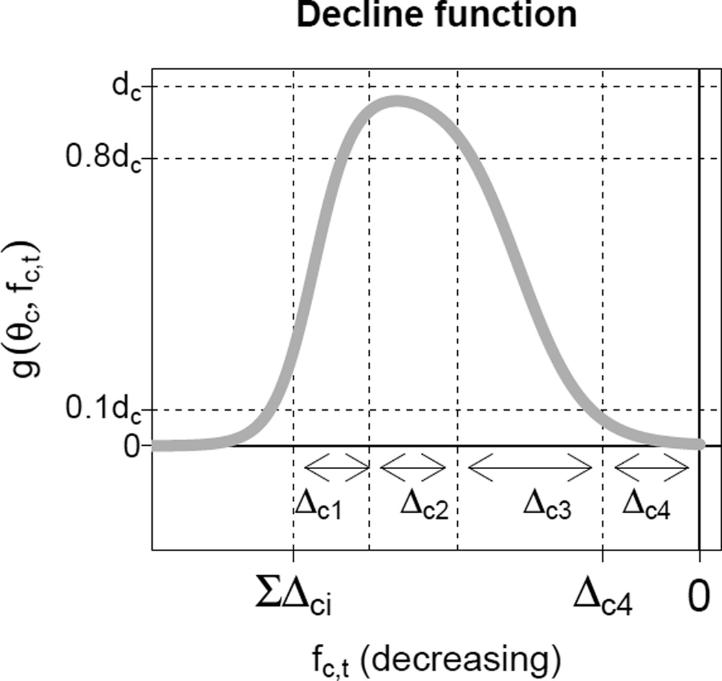
where g( , ) is a parametric decline function. This function specifies a five-year decrement (decrease) as a function of the current level of the TFR and parameter vector θ. The decline function is the sum of two logistic functions, i.e. a double logistic or bi-logistic function (United Nations, Department of Economic and Social Affairs, Population Division 2006). The double logistic function with country-specific parameter vector θ_c = (Δ_c1, Δ_c2, Δ_c3, Δ_c4, d_c), is given by

$$\frac{-d_c}{1+\text{exp }(-\frac{2\text{ln}(p_1)}{{\mathrm{\Delta }}_{c1}}(f_{c,t}-{\sum }_i{\mathrm{\Delta }}_{ci}+0.5{\mathrm{\Delta }}_{c1}))}+\frac{d_c}{1+\text{exp }(-\frac{2\text{ln}(p_2)}{{\mathrm{\Delta }}_{c3}}(f_{c,t}-{\mathrm{\Delta }}_{c4}+0.5{\mathrm{\Delta }}_{c3}))},$$

where d_c is the maximum possible pace of the decline, p₁ = p₂ = 9 are constants, and the Δ_ci’s describe the TFR ranges in which the pace of the fertility decline changes, where $U_c={\sum }_{i=1}^4{\mathrm{\Delta }}_{ci}$ is the start level of the fertility decline (see Figure 1).

Figure 1.

Five-year decrements as given by the double logistic decline function g(θ_c, f_c,t) plotted against the TFR. The horizontal TFR axis is negatively oriented (i.e. decreasing from left to right).

The parameters of the decline function are estimated for each country. For countries in which the start period τ_c of the fertility transition is within the observation period, the start level U_c is fixed at the TFR in that period, U_c = f_c,τc. For countries in which the transition started before the observation period, the start level is added as a parameter to the model, with prior distribution

$$U_c~U(\text{min}\{5.5,\underset{t}{\text{max}}{f}_{c,t}\},8.8).$$

Given U_c, the five parameters that determine the pace of the fertility decline and the time that the transition takes in country c are Δ_c4, {Δ_ci/(U_c − Δ_c4) : i = 1, 2, 3}, and d_c.

We use a Bayesian hierarchical model (Lindley and Smith 1972; Gelman et al. 2004) to estimate the parameters in each country. Transformations of parameters are used to restrict their outcomes to realistic values and for the purpose of computation. The Bayesian hierarchical model is given by:

$$d_c^{*}=\text{log }\left(\frac{d_c-0.25}{2.5-d_c}\right),$$

$$d_c^{*}~N(\chi ,{\psi }^2),$$

$${\mathrm{\Delta }}_{c4}^{*}=\text{log }\left(\frac{{\mathrm{\Delta }}_{c4}-1}{2.5-{\mathrm{\Delta }}_{c4}}\right),$$

$${\mathrm{\Delta }}_{c4}^{*}~N({\mathrm{\Delta }}_4,{\delta }_4^2),$$

$$p_{ci}=\frac{{\mathrm{\Delta }}_{ci}}{U_c-{\mathrm{\Delta }}_{c4}}\text{for }i=1,2,3,$$

$$p_{ci}=\frac{\text{exp}({\gamma }_{ci})}{{\sum }_{j=1}^3\text{exp}({\gamma }_{cj})},$$

$${\gamma }_{ci}~N({\alpha }_i,{\delta }_i^2),$$

with world-level mean and variance parameters {χ, ψ², Δ₄, δ₄, α, δ}. The prior distributions of these parameters are given in Appendix A.

To summarize, the country-specific parameters in the Phase II model are given by {γ_ci, U_c, d_c, Δ_c4}, i = 1, 2, 3. The hyperparameters are {χ, ψ², Δ₄, α_i, δ_i, δ₄} for i = 1, …, 3 and {a, b, S, σ₀, c₁₉₇₅, m_τ, s_τ}. An MCMC algorithm is used to get samples of the posterior distributions of each of the parameters of the fertility transition model (Gelfand and Smith 1990). This algorithm is a combination of Gibbs sampling, Metropolis-Hastings and slice sampling steps (Neal 2003).

2.2. Post-transition model

This phase of TFR change is modeled by a first order autoregressive time series model, an AR(1) model, with its mean fixed at the approximate replacement-level fertility, μ = 2.1:

$$f_{c,t+1}~N(\mu +\rho (f_{c,t}-\mu ),s^2)\text{ for }t\ge {\lambda }_c,$$ (3)

where ρ is the autoregressive parameter with |ρ| < 1 and s is the standard deviation of the random errors. Both parameters are estimated by maximum likelihood.

2.3. TFR projections

TFR projections during the fertility transition for countries that are currently in Phase II are based on the Phase II model (Section 2.1), using the sample from the posterior distribution of the model parameters.

Consider projecting f_c,t+1, the TFR in country c in period (t + 1), assuming that it is in Phase II in period t. The predictive distribution is represented by a sample $\{f_{c,t+1}^{(i)}:i=1,\dots ,I\}$. The i-th member of the sample, $f_{c,t+1}^{(i)}$, is given by $f_{c,t+1}^{(i)}=f_{c,t}^{(i)}-d_{c,t}^{(i)}+{\epsilon }_{c,t}^{(i)}$, where $f_{c,t}^{(i)}$ is the i-th member of the sample of TFR outcomes in period t, $d_{c,t}^{(i)}$ is the expected decrement given by the decline function evaluated at $f_{c,t}^{(i)}$ and ${\mathit{\theta }}_c^{(i)}$ (the i-th sample of parameter vector θ_c), and ${\epsilon }_{c,t}^{(i)}$ is a random draw from N(0, σ⁽ⁱ⁾(f_c,t)²).

For the countries that are currently in Phase II, the projected start of Phase III is given by the earliest period t such that (i) ${\text{min}}_t\{f_{c,t}^{(i)}\le {\mathrm{\Delta }}_{c4}^{(i)}\}$, and (ii) $f_{c,t}^{(i)}>f_{c,t-1}^{(i)}$. The projected start period will differ between trajectories because it depends on the expected fertility decrement (given by the decline parameters) and the random distortion term. For TFR projections of countries that are currently in Phase III, and the projections for a country that enters Phase III, the AR(1) model is used, as described in Section 2.2.

In all projections, an additional prior distribution is put on future TFR outcomes, f_c,t+1 ~ U[0, U_c]. The upper bound is used to exclude TFR trajectories in which the fertility transition does not take off. The lower bound ensures positive TFR outcomes. This prior is enforced by resampling any future distortion term that results in TFR outcomes outside its prior bounds. After constructing a large sample of TFR trajectories, the “best” TFR projection is given by the median outcome of the TFR trajectories in each period, and the bounds of the (1 − α)100% projection intervals are given by the α/2. 100th and (1 − α/2). 100th quantiles.

3. Using bayesTFR

We have implemented the methodology described above in an R package, called bayesTFR. This would be used by UN analysts and others whose task is to generate TFR projections including uncertainty bounds for all countries of the world.

To make probabilistic TFR projections using bayesTFR, the user will usually follow three basic steps in the following order:

1. Fit the TFR projection model:

   1. Calculate the start period of Phase II and the start period of Phase III for each country (τ_c and λ_c).
   2. Get a posterior sample of the Phase II model parameters using the MCMC algorithm.

2. Generate future TFR trajectories (this step includes estimating the parameters of the AR(1) model in Phase III using maximum-likelihood estimation).

3. Analyze the results using a set of functions that summarize, plot, diagnose and export results of the two steps above.

Depending on the size of the MCMC sample, steps 1(b) and 2 are expected to be relatively time-consuming. Thus, an analyst will usually perform these steps on different days or weeks. It is therefore important to ensure independence and durability of the results from the various steps and make the connectivity between steps as easy as possible. This is achieved by automatically storing results on the disk and by informing the user about their location, while giving the user the option of choosing the location.

The following sections describe the three steps above in more detail, using an example for a demonstration of the main package functions. Note that we chose to demonstrate the package on a realistic example, i.e. an example with a large number of MCMC iterations. Because running the functions of the first two steps can take several hours, it is not recommended to run the presented code as such when learning how to use the package. Users who wish to explore the functionality on a toy example should reduce the number of iterations to the order of magnitude of 10. Use help(function) for more specifics about each function described below and details about its arguments.

3.1. Fitting the TFR projection model

Fitting the TFR projection model is invoked by the function run.tfr.mcmc. The function uses historical time series of the TFR, provided by the United Nations and delivered as part of the package. Optional arguments start.year and present.year determine which year is the first year and the last year of the time series that should be included in the computation. As the name suggests, the main functionality is running the MCMC algorithm to obtain a posterior sample of Phase II model parameters. The calculation of the start period of Phase II and the start period of Phase III for each country is embedded within this function. This section discusses the details of the MCMC algorithm.

Starting a new simulation

Most arguments in the function run.tfr.mcmc refer to the parameters of the prior distributions of the hyperparameters described in Section 2.1, as well as the starting values of all model parameters (see Appendix A for default values on the priors). Although all additional arguments in run.tfr.mcmc have reasonable default values, there are a few arguments that a user will be most likely to modify; nr.chains determines the number of MCMC chains to run, iter sets the length of each MCMC, and output.dir is the location on disk where the results are written. Let us assume that the user wishes to have all results stored in a sub-directory of the current working directory, called “mylongrun”:

R> simulation.dir <- file.path(getwd(), 'mylongrun')

This directory will be used throughout the paper, with reference to it as the simulation directory.

Now, consider the following example:

R> m1 <- run.tfr.mcmc(nr.chains=5, iter=7000, output.dir=simulation.dir)

The call launches an MCMC simulation of five chains, 7,000 iterations each, with results stored in the simulation directory. Additional arguments include argument thin, which controls the thinning interval, e.g. thin = 5 means that every 5-th iteration is stored on disk (the default is no thinning). Argument seed can be used to fix the seed of the random number generator in order to assure reproducible results.

In addition to setting the argument iter to the desired length, the user can pass here the value “auto”. In such a case, the function attempts to automatically determine the length needed for convergence of the MCMC algorithm by adequate exploration of the posterior distribution. It first runs the simulation for a pre-defined number of iterations (by default three chains with 62,000 iterations each), then launches a procedure of convergence diagnostics using burnin 2000 and a thinning interval of 80 (see Section 3.3 for more details). If it results in a “not converged” state, it continues running the MCMCs. This is repeated until the simulation converges or a given number of repetitions is reached. All default settings for such an automatic simulation can be overwritten using the argument auto.conf.

At the end of the simulation, the simulation directory contains one sub-directory per chain, called “mcx” where x is an identifier of the chain. Each such sub-directory contains one text file per parameter. Names of the hyperparameters and their correspondence to the notation in Section 2 can be obtained from Table 1. All files contain one value per (thinned) iteration, except alpha and delta which contain three values per iteration. The full file names consist of the names in the table and the suffix “.txt”. Note that alphat_ i are not stored, since they can be computed on the y. Country-specific parameters are stored in one file per parameter and country. The correspondence of the file names and the notation in Section 2 is shown in Table 2. Each file has the suffix “_country code.txt”, with code being the UN country code which are 3-digit codes following ISO 3166-1 numeric standard. The gamma files contain three values per (thinned) iteration, the remaining ones contain one value per (thinned) iteration and the gammat_ i parameters are not stored. The model does not generate MCMCs for countries that are in Phase I.

Table 1.

Country-independent parameters from Section 2 with their corresponding names in the code. They can be obtained using tfr.parameter.names().

χ	ψ	Δ4	α1,2,3	δ1,2,3	δ4	$\frac{\text{exp}({\alpha }_i)}{{\sum }_j\text{exp}({\alpha }_j)}$
chi	psi	Triangle4	alpha	delta	delta4	alphat_i

a	b	S	σ0	c1975	mτ	sτ
a_sd	b_sd	S_sd	sigma0	const_sd	mean_eps_tau	mean_eps_tau

Table 2.

Country-specific parameters from Section 2 with their corresponding names in the code. They can be obtained using tfr.parameter.names.cs().

γc1,2,3	Uc	dc	Δc4	$\frac{\text{exp}({\gamma }_{ci})}{{\sum }_j\text{exp}({\gamma }_{cj})}$
gamma	U	d	Triangle_c4	gammat_i

Even though all the parameter files contain results from each (thinned) iteration, they are not necessarily written into files at each such iteration. Instead, they are collected in the memory, or a buffer. Argument buffer.size controls the number of iterations between two consecutive storing, i.e. the size of the buffer, and thus can make the simulation more runtime efficient. The larger the buffer.size, the fewer operations on disk. However, the larger the buffer.size, the more information can be lost in case of failure. The argument defaults to 100.

Meta information about the simulation is stored as a binary file, called “bayesTFR.mcmc.meta.rda”, in the main simulation directory. Furthermore, each “mcx” subdirectory contains meta information about the specific chain in a binary format. This file is called “bayesTFR.mcmc.rda”.

The function also supports parallel processing for running the individual chains on multiple processors, and thus achieve a speedup proportional to number of processors or chains. To use this functionality, argument parallel is set to TRUE and optionally set the argument nr.nodes to the required number of processors. By default, the function will launch each chain in a separate process. Thus, the above code can be sped-up by a factor of up to 5 by adding parallel=TRUE to the list of arguments. Note that this functionality requires the R package snowFT (Ševčíková and Rossini 2010) being installed.

As mentioned above, the estimation uses historical UN time series included in the package. One can overwrite all or some of the values with user-specific data. This can be achieved by using the argument my.tfr.file, which should point to a file of the structure described in Section 3.4.

Continuing an existing simulation

There are several reasons for wanting to continue running an existing simulation. For example, MCMC diagnostics might show that some parameters have not converged. Another reason could be an interrupted simulation due to a hardware or software failure. Given the computationally expensive nature of such simulations, starting a run from the beginning can lead to the loss of several days of computation in extreme situations.

Let us assume that we want to extend MCMCs created in the previous section by 1,000 iterations each. This can be done as follows:

R> m2 <- continue.tfr.mcmc(iter=1000, output.dir=simulation.dir)

At the end of processing this call, each chain will be 8,000 iterations long.

The function also allows the user to specify identifiers of chains to be continued, using the optional argument chain.ids. This feature can be especially useful if there is a failure when running the chains in parallel. In such a case, the chains will most likely be of different lengths and the continuation can be defined for each chain separately.

As when starting a new simulation, the arguments parallel and nr.nodes can be set to run the continuation in parallel, and the argument iter can be set to “auto” to combine the run with convergence diagnostics.

Accessing existing MCMC results

If at later time point it is desirable to access the MCMC results, this can be done as follows:

R> m3 <- get.tfr.mcmc(sim.dir=simulation.dir)

Here m3 is an object of class bayesTFR.mcmc.set (as is m1 and m2) that contains all information about the MCMC simulation, including a pointer to the disk where the parameter traces are stored. In this example, the object m3 is identical to the m2 object above.

To extract a specific chain out of the MCMC set, for example the second one, use

R> m3.chain2 <- tfr.mcmc(m3, chain.id=2)

which results in an object of class bayesTFR.mcmc. Similarly, function tfr.mcmc.list returns a list of such objects, corresponding to selected MCMC chains. Both objects from our examples, m3 and m3.chain2, can be used in various functions described in the following sections.

3.2. Generating projections

Generating new projections

After obtaining a posterior sample of the Phase II model parameters, as discussed in Section 3.1, one can generate a sample from the posterior distribution of future TFR trajectories for all the countries of the world, as described in Section 2.3, using the function tfr.predict. To create a TFR projection until 2100 from the results generated in Section 3.1, the user needs to pass the simulation directory where the MCMC results are stored (argument sim.dir), the end year of the projection (argument end.year), the MCMC burnin (argument burnin), and either a thinning interval (argument thin) or the number of trajectories to generate (argument nr.traj):

R> pred1 <- tfr.predict(sim.dir=simulation.dir, end.year=2100, burnin=2000,
                        nr.traj=3000, verbose=TRUE)

In this call, the function will remove 2,000 iterations from the beginning of each chain, and use 3, 000 equally-spaced parameter values out of the remaining 5 × 6, 000 = 30, 000 iterations in total for generating the trajectories. Setting the argument seed ensures reproducibility of the projections.

An optional logical argument use.diagnostics makes it possible to use the burnin and thinning interval from an existing convergence diagnostics object. This is especially useful if the MCMCs were generated using the iter="auto" option. The function automatically finds values of burnin and thin that led to a convergence of the simulation, and thus those arguments can be omitted.

The AR(1) parameters μ, ρ and s for the post-transitional phase as defined in Section 2.2 can be set by the user using the arguments mu, rho and sigmaAR1, respectively. The default outcomes are μ = 2.1, and the maximum-likelihood estimates for ρ and s.

The trajectories are stored in a binary format, by default in a sub-directory of sim.dir, called “predictions”. An argument output.dir can be given where another location can be specified. In the prediction directory, a binary file containing meta information is stored, called “prediction.rda”, and one binary file per country, containing all trajectories for each projection year, including the present year. These files are called “traj countrycode.rda” where code is the UN country code. In the example above, the number of future TFR outcomes would be 2, 000 × 19 values per file (because present.year in the run.tfr.mcmc function defaults to 2010 which gives 19 five-years projections). In addition, two summary comma-separated text files are created: One in a user-friendly format, called “projection summary user friendly.csv”, the other using a UN-specific coding, called “projection summary.csv”. Both files contain for each country in each projection period the median outcome, the lower and upper bounds of the 80% and 95% projection intervals, the median outcome plus/minus 0.5 child and a projection in which the TFR is kept constant.

Optionally, the projection function stores a sample of trajectories in a comma-separated text format which is called “ascii trajectories.csv”. The size of the sample can be controlled by the argument save.as.ascii which defaults to 1,000 trajectories. The trajectories are selected using equal spacing. No trajectories are saved in the text format if the argument is set to zero.

The projection function also saves the thinned MCMC traces (which were used to construct the projected trajectories) to disk. It allows the user to perform subsequent operations on the traces in timely efficient manner. The storage place is called “thinned_mcmc_thin_burnin” in the main simulation directory with thin and burnin being the actual values of thin and burnin, respectively, and it has the same structure as described in Section 3.1. If such thinned traces already exist (for example they could have been created by the convergence diagnostics procedure prior to this call, see Section 3.3), the step of constructing and storing the thinned traces is skipped and instead they are loaded from disk and directly used for generating the trajectories. This scenario is most likely to be used in combination with use.diagnostics being set to TRUE when the projection trajectories are to be generated on the same MCMC chains that passed the convergence test.

Finally, note that if the object m3 from Section 3.1 is available in our R environment, we can obtain the same projection results by replacing the argument sim.dir with the argument mcmc.set=m3 in the above call.

Accessing an existing projection

An existing projection, such as the one above, can be accessed by:

R> pred2 <- get.tfr.prediction(sim.dir=simulation.dir)

Here, pred2 is equal to pred1, which is an object of class bayesTFR.prediction. It contains all the information about the projection, including a pointer to the trajectories. The object can be passed to various functions for analyzing results, see Section 3.3.

3.3. Analyzing results

Summary functions

There are a few summary functions available in the package. To get summary information about the m3 object obtained as shown in Section 3.1, we can use

R> summary(m3, meta.only=TRUE)

MCMC parameters estimated for 196 countries.
Hyperparameters estimated using 196 countries.

WPP: 2008
Input data: TFR for period 1950 – 2010 .

Number of chains = 5
Iterations = 1 : 40000
Thinning interval = 1
Chains sample sizes: 8000, 8000, 8000, 8000, 8000

This gives meta information about the MCMC simulation. Setting meta.only to FALSE will give more detailed information about the hyperparameters, using the summary function of the coda package (Plummer et al. 2010). For getting the same information about the country-specific parameters, it is advisable to do it for a specific country, using the argument country which is either the name or the numerical UN code of the country. The thinning interval and length of burnin can be controlled by the arguments thin and burnin, respectively. Furthermore, one can set the argument chain.id to a specific MCMC chain identifier to get information about one specific chain, or pass the one-chain object, such as m3.chain2, directly to the summary function. Further arguments, par.names and par.names.cs, respectively, can be set to restrict the summary information to specific parameters, country-independent and country-specific, respectively (see Tables 1 and 2 for the specific names). For example, the following command gives information only about the parameters specific to Ireland, and not about the hyperparameters:

R> summary(m3, country='Ireland', par.names=NULL, thin=10, burnin=2000)

...

Country: Ireland

Iterations = 2010:8000
Thinning interval = 10
Number of chains = 5
Sample size per chain = 600

1. Empirical mean and standard deviation for each variable,
   plus standard error of the mean:

                    Mean      SD  Naive SE Time-series SE
U_c372           7.13182 0.93419 0.0170558       0.017998
d_c372           0.11762 0.03656 0.0006675       0.001117
Triangle_c4_c372 1.62505 0.21343 0.0038967       0.005596
gammat_1_c372    0.08643 0.09264 0.0016913       0.002850
gammat_2_c372    0.28125 0.19192 0.0035039       0.007104
gammat_3_c372    0.63232 0.20714 0.0037818       0.008716

2. Quantiles for each variable:

                     2.5%     25%     50%    75%  97.5%
U_c372           5.599465 6.33729 7.13513 7.9244 8.7063
d_c372           0.067479 0.09007 0.11023 0.1384 0.2092
Triangle_c4_c372 1.234277 1.47621 1.61336 1.7699 2.0551
gammat_1_c372    0.007388 0.03000 0.05798 0.1043 0.3424
gammat_2_c372    0.031371 0.13053 0.23380 0.3973 0.7309
gammat_3_c372    0.189780 0.49025 0.66663 0.7999 0.9375

Note that in the default settings parameters γ_ci and α_i (i = 1, 2, 3) are considered only in their transformed form. This is because the signature of the summary function defines the MCMC parameters as follows:

function(..., par.names = tfr.parameter.names(trans=TRUE),
              par.names.cs = tfr.parameter.names.cs(trans=TRUE),
         ...)

To include also parameters on the original scale, remove the trans argument (or equivalently set it to NULL). The value trans=FALSE means that only parameters on the original scale are considered.

Another summary function is available for prediction objects. Using the pred2 object obtained as shown in Section 3.2, we can get statistics about the projected trajectories, starting with the last observed period (periods are denoted by their midyear):

R> summary(pred2, country='Czech Republic')

Projections: 18 ( 2013 – 2098 )
Trajectories: 3000
Burnin: 2000
Parameters of AR(1):
  mu   rho  sigma
 2.1 0.906 0.0922

Country: Czech Republic
Projected TFR:
     mean     SD 2.5%   5%  10%  25%  50%  75%  90%  95%97.5%
2008 1.41 0.0000 1.41 1.41 1.41 1.41 1.41 1.41 1.41 1.41 1.41
2013 1.48 0.0922 1.30 1.33 1.36 1.41 1.48 1.54 1.60 1.63 1.66
2018 1.54 0.1238 1.30 1.33 1.38 1.45 1.54 1.62 1.70 1.74 1.78
2023 1.59 0.1425 1.31 1.36 1.40 1.50 1.59 1.69 1.77 1.83 1.87
2028 1.64 0.1566 1.32 1.38 1.44 1.53 1.64 1.74 1.84 1.90 1.95
2033 1.68 0.1702 1.34 1.40 1.47 1.57 1.68 1.80 1.90 1.96 2.02
2038 1.72 0.1810 1.37 1.43 1.49 1.60 1.72 1.85 1.96 2.02 2.07
...

Setting an optional argument compact to FALSE will extend the set of quantiles to a larger set.

Exploring TFR trajectories

In addition to the summary function that gives commonly used quantiles of the trajectories, one can plot the posterior sample of trajectories, including user-defined projection intervals. For example,

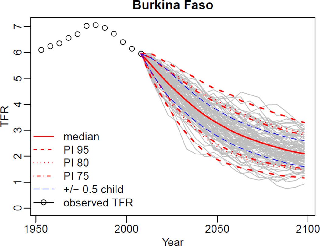
R> tfr.trajectories.plot(pred2, country='Burkina Faso', pi=c(95, 80, 75),
                         nr.traj=100)

shows the median outcomes, and lower and upper bounds of the 95, 80 and 75% projection intervals (see Figure 2). In addition, the graph includes the median outcomes +/− 0.5 child. This variant can be turned off by setting the argument half.child.variant=FALSE. The number of trajectories displayed is controlled by the argument nr.traj. Note that nr.traj in this function only influences the display – the quantiles included in the graph are computed using trajectories defined in the tfr.predict function (see Section 3.2), in our case 3, 000.

Figure 2.

Projected trajectories for Burkina Faso.

The same information in a tabular form can be obtained using:

R> tfr.trajectories.table(pred2, country='Burkina Faso', pi=c(95, 80, 75))

Its output is similar to the one from the summary function, except that it includes user-defined projection intervals and the historical time series.

If it is of interest to create trajectory graphs for all countries at once, one can use:

R> tfr.trajectories.plot.all(pred2, output.dir='trajplotall', nr.traj=100,
                             output.type='pdf', verbose=TRUE)

This creates one pdf-file per country in the directory called “trajplotall”. In addition to “pdf”, other possible output types are “png”, “jpeg”, “bmp”, “tiff”, or “postscript”.

Posterior distribution of the double logistic function

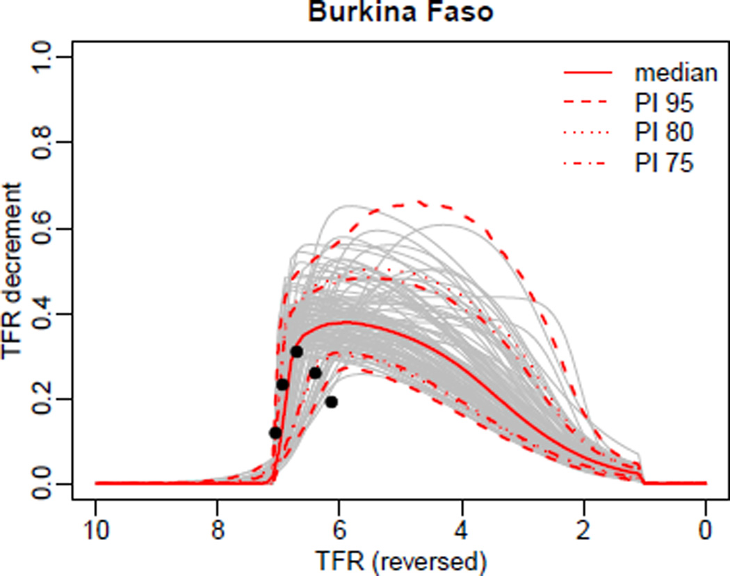
The posterior results for the double logistic function (DLF) as defined in Equation (2) can be viewed using:

R> DLcurve.plot(country='Burkina Faso', mcmc.list=m3, burnin=2000,
                pi=c(95,  80, 75), nr.curves=100)

The output is shown in Figure 3. The function argument mcmc.list is a pointer to the five MCMC chains from our example run. Alternatively, it can be a list of selected chains (result of tfr.mcmc.list), just a single MCMC chain (such as m3.chain2), or a prediction object (such as pred1 and pred2).

Figure 3.

Visualization of the posterior distribution of the double logistic function for Burkina Faso.

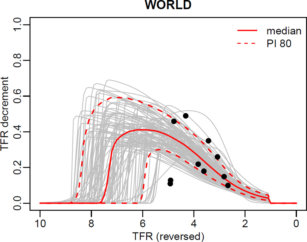
In the figure, the median outcomes and projection intervals of the DLF that are shown are calculated based on the sample of posterior DLFs, namely the DLFs that are given by the (thinned) iterations of the given chains, after removing the user-specified number of burnin iterations from each chain. For time-efficiency, a maximum of 2,000 DLFs are computed. The projection intervals are given by the corresponding quantiles of the posterior sample of DLFs on a fine grid of TFR outcomes. For the display, a number of curves given by nr.curves are selected using equal spacing and plotted. The observed 5-year decrements are also shown in the graph as filled circles.

The DLF graphs can be created for all countries at once using:

R> DLcurve.plot.all(m3, output.dir='DLplotall', nr.curves=100,
                    output.type='pdf', burnin=2000, verbose=TRUE)

Again, it creates one pdf-file per country in the directory called “DLplotall”, and the output.type argument can be changed to one of “png”, “jpeg”, “bmp”, “tiff”, and “postscript”.

TFR world map

The package supports creating world maps for any projection period and quantile of the posterior sample of TFR trajectories. It is based on the R package rworldmap (South 2010), which in turn uses among others the package fields (Furrer et al. 2010) for creating a nice legend. It allows user-defined settings of the coloring scheme. Calling simply

R> tfr.map(pred2)

creates a world map of the TFR in the last observed time period, in heat colors as the default. The user can pass further optional arguments, such as quantile=p for the p·-100th quantile, with 0 ≤ p ≤ 1, or projection.year to specify the projection time which is given as the middle year of a projection period, e.g. 2013 for the period 2010–2015 or 2018 for the period 2015–2020. Furthermore, any arguments of the rworldmap function mapCountryData can be passed to the tfr.map function, to change the display. In order to control the map device, the tfr.map function has an argument device which can be any device type, such as “png”, “pdf”, etc. In the default setting (device=‘dev.new‘), a new graphical device pops up every time this function is called. An argument device.args is a list of arguments passed to the chosen device (see help on mapDevice of rworldmap).

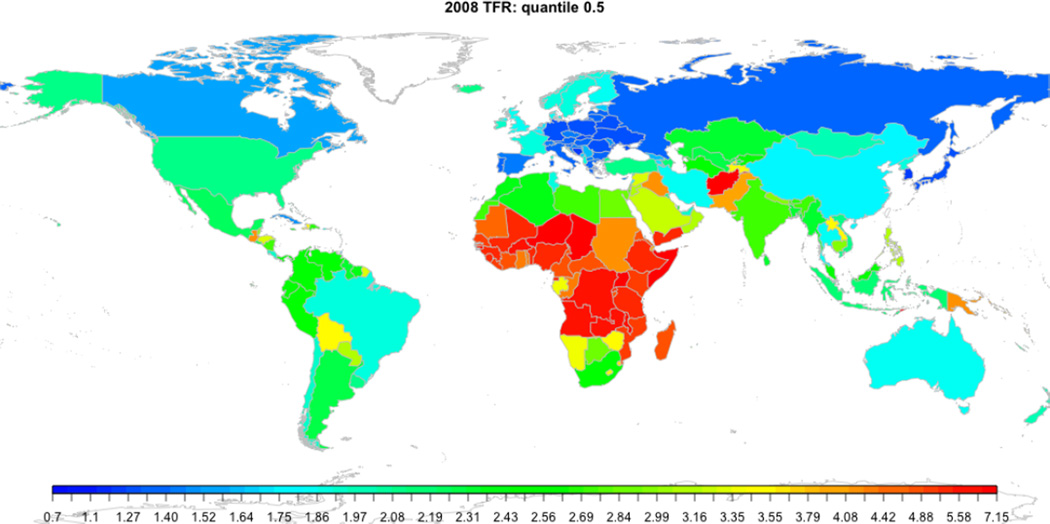
The bayesTFR package offers a function for automatically assembling graphical parameters and tfr.map arguments. The function is called get.tfr.map.parameters. For example, the following code generates the map in Figure 4:

R> params <- get.tfr.map.parameters(pred2)
R> do.call('tfr.map', params)

The color scheme follows quantiles of a Gamma distribution estimated from the last observed TFR, here the displayed TFR. It defaults to 50 color categories which can be changed using the argument nr.cats. Any other arguments that the tfr.map function accepts can be passed to get.tfr.map.parameters.

Figure 4.

World map visualizing the TFR in 2005–2010 in each country.

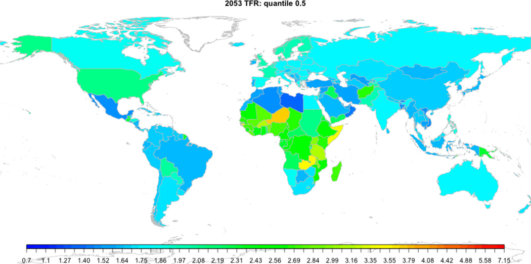
This way of creating the graphical parameters has the advantage that we can now use params from the previous example to generate maps for other projection periods on the same scale. For example

R> do.call('tfr.map', c(list(projection.year=2053, device='png',
            device.args=list(width=1000, file='worldTFR2053.png')), params))
R> dev.off()

creates a png-file, shown in Figure 5, which has the same color scale as Figure 4. If the maps do not have to be on the same scale, one can set the argument same.scale=FALSE in get.tfr.map.parameters.

Figure 5.

World map visualizing the median TFR projection in 2050–2055 in each country.

To generate world maps from all projection periods at once, the command

R> tfr.map.all(pred2, output.dir='tfrmaps', output.type='pdf')

creates a set of maps in pdf-format in the directory “tfrmaps”. Any argument mentioned above can be passed here, such as quantile, nr.cats, same.scale or any argument of the tfr.map function.

MCMC parameter traces

The traces of the MCMC parameters can be graphically explored using two functions: one for plotting country-independent parameters, the other for plotting country-specific parameters. Using our example,

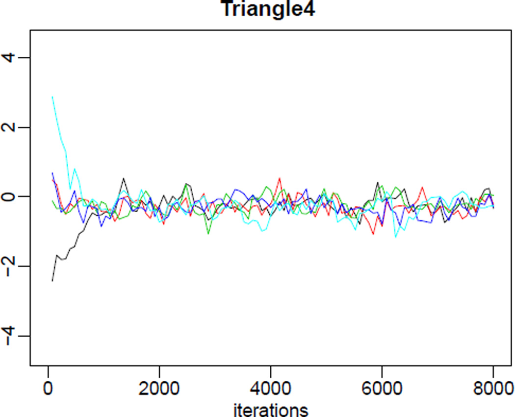
R> tfr.partraces.plot(mcmc.list=m3, par.names='Triangle4', nr.points=100)

will create a graph for parameter Δ₄, containing one trace per MCMC chain (in our example five traces), as shown in Figure 6. The argument nr.points (or optionally thin) controls the number of points plotted in each trace. One could also remove the burnin period from the plot using the argument burnin, or pass any graphical parameters, such as xlim or ylim. The argument par.names can contain any subset of the names in Table 1 to be plotted; leaving out the argument will create a graph for each country-independent parameter. In addition to the name alpha, one can use alpha_i (i = 1, 2, 3) to get traces for a specific value of i. The same applies to its transformed equivalents.

Figure 6.

Parameter traces for the parameter Δ₄, generated via the simulation in Section 3.1.

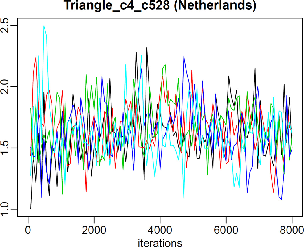
Plotting country-specific parameters is done analogously, using the function tfr.partraces.cs.plot. The graph in Figure 7 was generated using

R> tfr.partraces.cs.plot(country='Netherlands', mcmc.list=m3, nr.points=100,
                         par.names='Triangle_c4')

An optional argument chain.ids can be passed to both functions if traces from specific MCMC chains are to be plotted.

Figure 7.

Parameter traces for the country-specific parameter Δ_c4 for the Netherlands, generated via the simulation in Section 3.1.

Posterior distribution of the model parameters

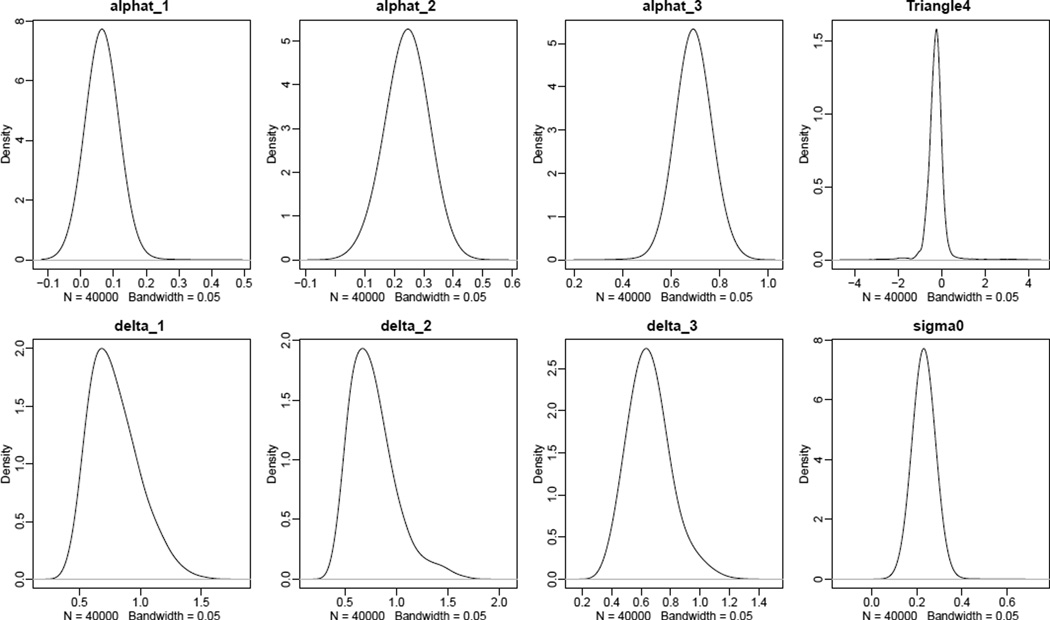
The density of the posterior distribution of the MCMC parameters can be viewed using the functions tfr.pardensity.plot (for country-independent parameters) and tfr.pardensity.cs.plot (for country-specific parameters). Optional arguments par.names and chain.ids have the same meaning as in the case of plotting parameter traces in the previous section. The following code was used to generate Figure 8:

R> tfr.pardensity.plot(pred2,
                       par.names=c('alphat', 'Triangle4', 'delta', 'sigma0'),
                       dev.ncol=4, bw=0.05)

If passing a prediction object as the first argument, the posterior distribution is plotted using the same thinned MCMCs that were used for generating the projection trajectories, in this example of length 3, 000. Alternatively, one can pass a set of MCMCs, such as our objects m2 or m3, in which case the distribution is constructed using all stored iterations. Here, setting an argument burnin can be useful in order to discard the burnin iterations.

Figure 8.

Density of the posterior distribution of various country-independent parameters.

The dev.ncol argument controls the number of plots per row and the bandwith argument bw is passed to the underlying density function. Function tfr.pardensity.cs.plot is used in the same way, except that country must be given as the first argument to specify for which country the density of country-specific parameters should be plotted.

MCMC convergence diagnostics

The package provides a convenient all-in-one function for determining convergence of the simulated MCMC chains, called tfr.diagnose, as well as a lower-level diagnostic function with the possibility of various user-defined settings, called tfr.raftery.diag. Here, we only explain the main functionality; for more information see the help-file of those functions.

The main results in the functions are based on the run length diagnostic of Raftery and Lewis (1992b,a, 1996), as implemented in raftery.diag in the coda package (Plummer et al. 2010). This function is repeatedly called for different sets of parameters and its results are bundled together.

To run convergence diagnostics on chains stored in the simulation directory using 2000 iterations as burnin and 10 iterations as the thinning interval, one can use

R> diag <- tfr.diagnose(simulation.dir, thin=10, burnin=2000)

The function stores the resulting object on disk, in a sub-directory of simulation.dir called “diagnostics” with file name being “bayesTFR.convergence 10 2000.rda”. The numbers 10 and 2000 in the file name are the values of the argument thin and burnin, respectively.

To obtain diagnostics results stored on disk, use

R> diag2 <- get.tfr.convergence(simulation.dir, thin=10, burnin=2000)
R> summary(diag2)

...
Convergence checked on 196 countries out of 196 countries total.

Simulation has converged.
Number of trajectories to be used: 3000
Status: green

In this example, diag and diag2 contain the same data.

If the diagnostic suggests that the chains converged, as in our case, it gives a suggestion how many projection trajectories to generate, which is simply the total number of iterations (after removing burnin) divided by the thinning interval. This number can be then passed to the tfr.predict function as the argument nr.traj. If the chains did not converge, the function gives a recommendation, how many more iterations to run to achieve convergence.

To find diagnostics objects for all combinations of thin and burnin available on disk, run

R> diag.list <- get.tfr.convergence.all(simulation.dir)

which returns a list of all such objects.

The tfr.diagnose function proceeds as follows to determine if the simulation has run long enough:

1. For each parameter j and each MCMC chain i remove the given burnin and thin by the given thinning interval.

2. Run raftery.diag with arguments r=0.0125 and q=0.025 on each of those arrays and obtain the value of N_0.025(i, j) which is the estimated unthinned length of chain i for parameter j.

3. Obtain the median of N_0.025(i, j) over all chains i, say Ñ_0.025(j).

4. The same as 2. with changing the q argument to q=0.975, obtain N_0.975(i, j) and its median over chains Ñ_0.975(j).

5. Take N̂ = max_j{Ñ_0.025(j), Ñ_0.975(j)} and compare with the total number of iterations that your simulation contains, i.e. summed over all chains after removing burnin from each chain.

The function results in a state “not converged” (or “red”) if N̂ is larger than the total number of iterations, or in a state “converged” (or “green”) otherwise.

If the optional logical argument keep.thin.mcmc of tfr.diagnose is set to TRUE, the thinned traces used in the diagnostics procedure, collapsed into one chain, are stored on disk. They are then automatically found and used by the tfr.predict function, if called with the same thin and burnin (see Section 3.2).

The functions run.tfr.mcmc and continue.tfr.mcmc offer the option of combining an MCMC simulation with convergence diagnostics, by setting the argument iter="auto". In such a simulation, the diagnostics object is computed (using burnin=2000 and thin=80 as defaults) and stored automatically during the simulation, possibly multiple times, until convergence. Then, the tfr.predict function can be called with use.diagnostics=TRUE in which case the number of trajectories and burnin is automatically determined from the diagnostics object.

3.4. Using user-specific data

As mentioned in previous sections, the estimation functions use historical UN time series included in the package. One can use the data function to explore those data:

R> data('UN2008')
R> colnames(UN2008)

 [1] "Index"     "country"   "country_code" "1950–1955" "1955–1960"
 [6] "1960–1965" "1965–1970" "1970–1975"    "1975–1980" "1980–1985"
[11] "1985–1990" "1990–1995" "1995–2000"    "2000–2005" "2005–2010"
[16] "2010–2015" "2015–2020" "2020–2025"    "2025–2030" "2030–2035"
[21] "2035–2040" "2040–2045" "2045–2050"

However, it is sometimes of interest to supply user-specific data for one or more countries. Such a file, say my_tfr_file, should have the same structure as the UN2008 data, i.e. one row per country and columns containing the TFR in different time periods. The only required column is country_code containing the UN 3-digit codes of countries. Values in this column should be contained in the UN lookup table, called WPP2008_LOCATIONS:

R> data('WPP2008_LOCATIONS')
R> # list all available countries and their aggregations
R> WPP2008_LOCATIONS[,2:3]

The estimation function will overwrite the default UN data by any TFR columns supplied in my_tfr_file for the given countries. For example, if my_tfr_file contains

"country_code" "country" "2005–2010"
  124          "Canada"      1.5

the estimation will use the UN time series for Canada for all time periods except 2005–2010 where it is replaced by 1.5.

my_tfr_file also allows two additional columns, namely last.observed which serves the purpose of dealing with missing data and will be discussed in Section 3.6, and include_code which is significant for estimation and aggregations. include_code can have three different values:

• 2: Country is included in the MCMC estimation (as described in Section 3.1).

• 1: Country is not included in the MCMC estimation, i.e. it does not have any influence on the posterior sample of hyperparameters and thus the posterior samples of parameters for the other countries. Projections for such a country are still possible; a sample of the posterior distributions of its parameters is obtained based on the posterior sample of the model hyperparameters. This can be useful for example for countries with unusual historical pattern of TFR, or in case of aggregated TFR outcomes for subsets of countries, which will be discussed in more detail in Section 3.5.

• 0. Country is ignored.

The default values for include_code are taken from WPP2008_LOCATIONS and are overwritten by those supplied in my_tfr_file. See for example countries that are by default included in the estimation:

R> WPP2008_LOCATIONS[WPP2008_LOCATIONS[,'include_code']==2,2:3]

The package contains a template of my_tfr_file, called “my_tfr_template.txt”, located in the data directory.

3.5. Aggregations

The UN data file of historical TFR time series contains TFR outcomes for subsets of countries, for example for specific areas, continents or the whole world. By default include_code in WPP2008_LOCATIONS is set to 0 for any aggregated area, which means aggregations are ignored in the estimation process. However, it is often of interest to obtain projections of aggregated TFR outcomes for these areas. We implemented a simple approach to obtain the projections for these aggregates: Treat the aggregated countries as a “new country” (without including it in the MCMC estimation). In this approach, the posterior sample of the hyperparameters (from Table 1) is used to generate a posterior sample of the country-specific parameters for the aggregation¹.

The posterior sample for aggregate-specific parameters can be obtained in two ways in the bayesTFR package; during the initial MCMC simulation described in Section 3.1, or afterwards. The former saves computation time while the latter allows for generating projections for additional aggregations that were not considered at the time of the initial simulation. In the first approach, the user has to overwrite the include_code values of the aggregates using a user-defined file that includes the include_code column, as discussed in Section 3.4. Typically, one would set the include_code for such aggregates to 1, which means that only country/aggregation-specific parameters are to be estimated. For example, to run the MCMC simulation that includes “World” without “World” having an impact on the hyperparameters, one can create a file containing just one line of data:

"country_code" "country" "include_code"
900            "WORLD"          1

If user-specific historical TFR values are to be used, additional columns with the specific time period headers can be added. Passing the name of this file into the run.tfr.mcmc function as the my.tfr.file argument will generate aggregate-specific parameters for the aggregation “World”. The user can then proceed as usual with generating projections as described in Section 3.2 – “World” will be automatically included in the set of countries for which future TFR trajectories are created. It is advisable to include all aggregations for which projections are needed into the user-defined TFR file, as the second approach of dealing with aggregations requires additional steps.

If an MCMC run has already finished and we wish to make projections for aggregated TFR outcomes for the aggregate that was not included in my_tfr_file, a posterior sample of the aggregate-specific parameters like above can be obtained with the command

R> m4 <- run.tfr.mcmc.extra(simulation.dir, countries=900)

which uses random draws from the posterior samples of the hyperparameters stored in simulation.dir to sample the aggregate-specific parameters for the subsets of countries with UN code given by the argument countries, here 900 which is “World”. The next step is to generate projections. If projections have already been generated for the countries that were included in the first run (that was stored in simulation.dir) before creating m4, one can save computation time by using

R> pred3 <- tfr.predict.extra(simulation.dir, save.as.ascii=0)

This call checks which countries/subsets of countries have posterior samples of the model parameters, but no projections, and generates projections for these countries/subsets of countries. Then one can examine the results as usual using

R> summary(m4, country=900, par.names=NULL)
R> summary(pred3, country=900)
R> tfr.trajectories.plot(pred3, country=900, nr.traj=100)
R> DLcurve.plot(country=900, mcmc.list=m4, burnin=2000, nr.curves=100)

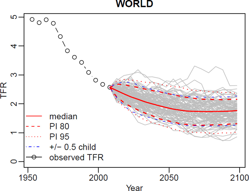
Results of the last two calls are shown in Figures 9 and 10.

Figure 9.

Projected trajectories for the world.

Figure 10.

Posterior distribution of the double logistic function for the world.

3.6. Imputing missing values

The TFR data set that is included in the package (UN2008) gives the UN estimates from 1950–1955 until 2005–2010 for all countries. For a number of countries the most recent entries are not actually observed – they are estimated based on UN methodology (United Nations, Department of Economic and Social Affairs, Population Division 2006). The package allows the user to exclude these periods when fitting the projection model, and to construct estimates for the missing periods based on the estimated model parameters. In this approach, the last observation period is changed to the last period in which TFR data was available, and projections start from that period.

Information about the last observed data point for each country is included in the package, in a file called “UN2008_with_last_obs.txt” located in the data directory.² This file has the same structure as the UN2008 data, except that it has an additional column called last.observed containing the year of the last observation in each country. Thus, we can treat the TFR data starting from that year and later as missing. If the year of the last observed data point is greater than or equal to t_i + 3, the missing time periods start at the period [t_i+1, t_i+2]. If it is smaller than t_i + 3, it starts one period earlier, namely [t_i, t_i+1]. Similarly, the user can provide her/his own TFR file as described in Section 3.4 with the column last.observed included.

To use the UN file and let the model impute the missing estimates, we can run the following code:

R> simulation.dir.miss <- file.path(getwd(), 'runwithmissingdata')
R> my.tfr.file <- file.path(.find.package('bayesTFR'),
                           'data', 'UN2008_with_last_obs.txt')
R> m5 <- run.tfr.mcmc(nr.chains=5,  iter=8000, output.dir=simulation.dir.miss,
                      my.tfr.file=my.tfr.file)
R> pred4 <- tfr.predict(sim.dir=simulation.dir.miss, end.year=2100,
                        burnin=2000, nr.traj=3000, verbose=TRUE)

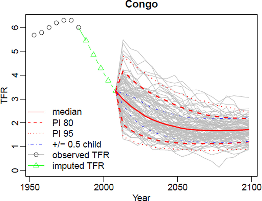
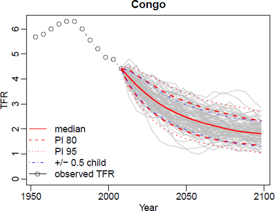
In the above commands, we set a different simulation directory in order not to overwrite our previously generated results. Then we pass the TFR file included in the package into the MCMC estimation. The resulting m5 object is equivalent to the m2 and m3 objects, except that the missing data were not included in the estimation. The result of the projection generation, pred4, is equivalent to the pred1 and pred2 objects except that missing data are replaced by the median of the generated trajectories. See Figure 11 for an example of generated trajectories for Congo using the pred4 object. The imputed values are marked by a green line. For comparison, Figure 12 shows the corresponding plot created from the pred2 object, i.e. without considering missing data. As can be seen, imputing missing values increases the uncertainty bounds. Note that in this simulation, six countries were excluded from the MCMC estimation, since their last observed data points indicated being in Phase I. This information can be obtained from summary of the m5 object.

Figure 11.

Projected trajectories for Congo with missing data imputed by the projection model. The last observation year for Congo is 1985. The plot was created using the object pred4.

Figure 12.

Projected trajectories for Congo without missing data, i.e. the UN estimates are considered as observed TFRs. The plot was created using the object pred2.

4. Graphical user interface

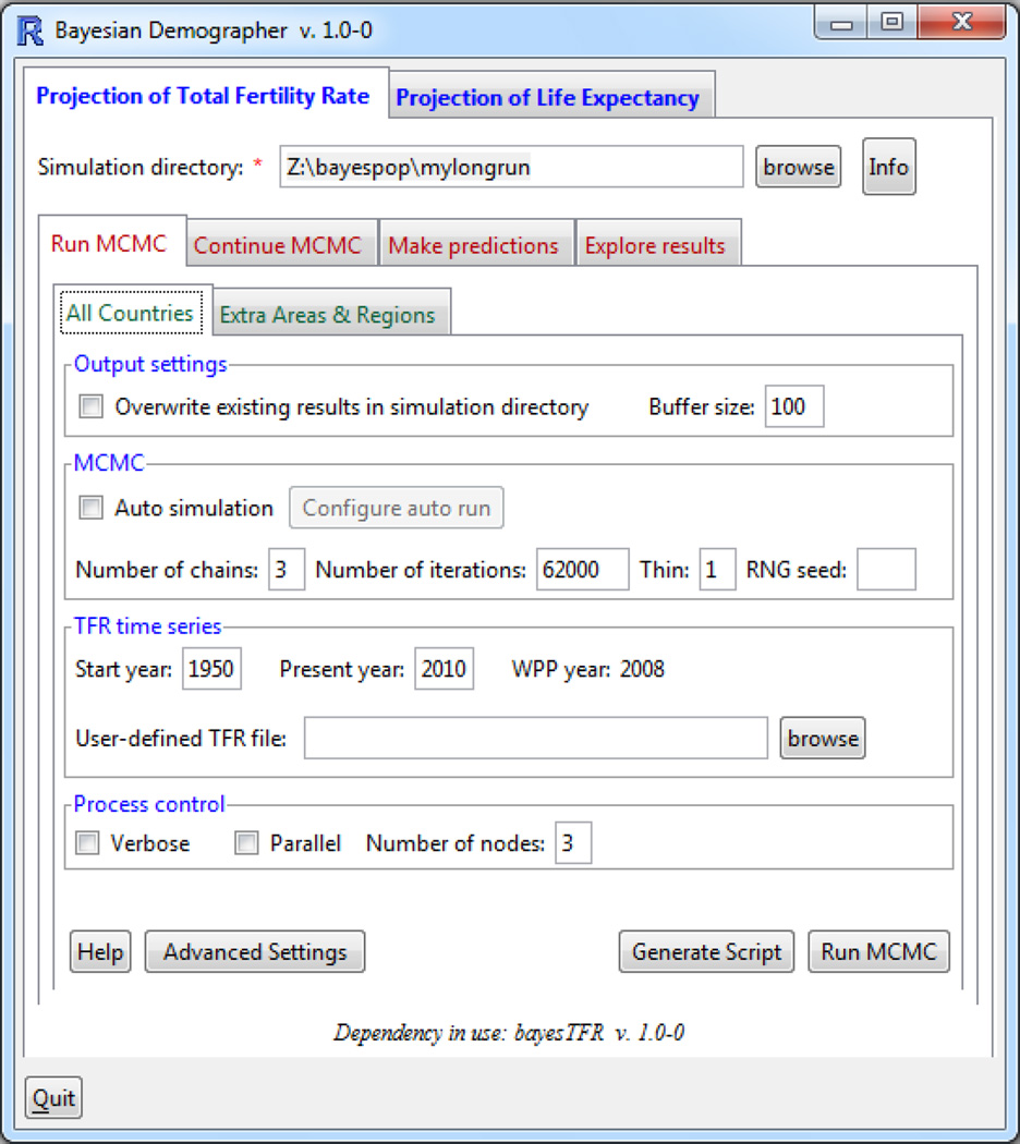
We have developed a graphical user interface (GUI) for the bayesTFR package, also as an R package called bayesDem. Its design follows the described workflow as a set of tabs, starting at the left with running the MCMC algorithm, and continuing to the right with “Continue MCMC”, generating projections and exploring results, see Figure 13. Each tab is usually divided into sub-tasks, implemented again as tabs. For example, the “Run MCMC” tab in the figure contains one tab for fitting the Phase II model for all countries as described in Section 3.1 and another tab for obtaining posterior samples of model parameters for aggregations, called “Extra Areas & Regions”. Each tab contains a “Generate Script” button that provides the corresponding bayesTFR commands with all argument values from the GUI filled in. Thus, by copying and pasting the user can easily create a batch file of various tasks conveniently from the GUI. Almost all features of the package described in this paper can be accessed through the GUI, including generating plots and maps, or running and exploring convergence diagnostics.

Figure 13.

Graphical user interface for bayesTFR, from the package bayesDem.

Appendix

A. Prior distributions

The prior distributions on the variance parameters {a, b, S, σ₀, c₁₉₇₅, m_τ, s_τ}, defined in Section 2.1, are given by:

$$a~U[a_l,a_u],$$

$$b~U[b_l,b_u],$$

$${\sigma }_0~U[{\sigma }_l,{\sigma }_u],$$

$$c_{1975}~U[c_l,c_u],$$

$$S~U[S_l,S_u],$$

$$m_{\tau }~N(m_0,s_0^2),$$

$$1/s_{\tau }^2~\text{Gamma}(1,s_0^2).$$

The correspondence of these parameters to their argument names and default values used in bayesTFR version 1.0-0 is shown in the following tables.

notation	al	au	bl	bu	σl	σu
argument name	a.low	a.up	b.low	b.up	sigma0.low	sigma0.up
default value	0	0.2	0	0.2	0.01	0.6

notation	cl	cu	Sl	Su	m0	s0
argument name	const.low	const.up	S.low	S.up	mean.eps.tau0	sd.eps.tau0
default value	0.8	2	3.5	6.5	−0.25	0.4

The prior distributions on the world-level mean and variance parameters {χ, ψ², Δ₄, δ₄, α, δ} is given by:

$$\chi ~N({\chi }_0,{\psi }_0^2),$$

$$1/{\psi }^2~\text{Gamma}(1,{\psi }_0^2),$$

$${\alpha }_1~N({\alpha }_{0.1},{\delta }_0^2),$$

$${\alpha }_2~N({\alpha }_{0.2},{\delta }_0^2),$$

$${\alpha }_3~N({\alpha }_{0.3},{\delta }_0^2),$$

$$1/{\delta }_i^2~\text{Gamma}(1,{\delta }_0^2),\text{ for }i=1,\dots ,3$$

$$1/{\delta }_4^2~\text{Gamma}(1,{\delta }_{4.0}^2),$$

$${\mathrm{\Delta }}_4~N({\mathrm{\Delta }}_{4.0},{\delta }_{4.0}^2).$$

with their correspondence to argument names and default values:

notation	χ0	ψ0	α0.p	δ0	δ4.0	Δ4.0
argument name	chi0	psi0	alpha0.p	delta0	delta4.0	Triangle4.0
default value	−1.5	0.6	−1, 0.5, 1, 5	1	0.8	0.3

References

- Alkema L, Raftery AE, Gerland P, Clark SJ, Pelletier F, Buettner T. Working Paper of the Center for Statistics and the Social Sciences. Vol. 97. University of Washington; 2010. Probabilistic Projections of the Total Fertility Rate for All Countries. URL http://www.csss.washington.edu/Papers. [Google Scholar]
- Alkema L, Raftery AE, Gerland P, Clark SJ, Pelletier F, Buettner T. Probabilistic Projections of the Total Fertility Rate for All Countries. To appear in Demography. 2011 doi: 10.1007/s13524-011-0040-5. [DOI] [PMC free article] [PubMed] [Google Scholar]
- Furrer R, Nychka D, Sain S. fields: Tools for spatial data. R package version 6.3. 2010 URL http://CRAN.R-project.org/package=fields. [Google Scholar]
- Gelfand A, Smith AFM. Sampling-based approaches to calculating marginal densities. Journal of the American Statistical Association. 1990;85:398–409. [Google Scholar]
- Gelman A, Carlin JB, Stern HS, Rubin DB. Bayesian Data Analysis. 2nd. Boca Raton, Fl: Chapman & Hall/CRC; 2004. [Google Scholar]
- Lindley DV, Smith AFM. Bayes Estimates for the Linear Model. Journal of the Royal Statistical Society B. 1972;34:1–41. [Google Scholar]
- Neal RM. Slice sampling. The Annals of Statistics. 2003;31(3):705–767. [Google Scholar]
- Plummer M, Best N, Cowles K, Vines K. coda: Output analysis and diagnostics for MCMC. R package version 0.13–5. 2010 URL http://CRAN.R-project.org/package=coda. [Google Scholar]
- R Development Core Team. R: A Language and Environment for Statistical Computing. Vienna, Austria: R Foundation for Statistical Computing; 2010. ISBN 3-900051-07-0, URL http://www.R-project.org. [Google Scholar]
- Raftery A, Lewis S. One long run with diagnostics: Implementation strategies for Markov chain Monte Carlo. Statistical Science. 1992a;7:493–497. [Google Scholar]
- Raftery AE, Lewis SM. How many iterations in the Gibbs sampler? In: Bernardo JM, et al., editors. Bayesian Statistics 4. Oxford University Press; 1992b. pp. 763–773. [Google Scholar]
- Raftery AE, Lewis SM. Implementing MCMC. In: Gilks WR, Spiegelhalter DJ, Richardson S, editors. Markov Chain Monte Carlo in Practice. Chapman and Hall, London: 1996. pp. 115–130. [Google Scholar]
- South A. rworldmap: For mapping global data : rworldmap. R package version 0.107. 2010 URL http://CRAN.R-project.org/package=rworldmap. [Google Scholar]
- United Nations, Department of Economic and Social Affairs, Population Division. World Population Prospects. The 2004 Revision, Vol. III, Chapter VI. Methodology of the United Nations population estimates and projections. 2006:100–104. http://www.un.org/esa/population/publications/WPP2004/WPP2004_Volume3.htm.
- United Nations, Department of Economic and Social Affairs, Population Division. World Population Prospects. The 2008 Revision. United Nations publication. 2009 URL http://www.un.org/esa/population/publications/wpp2008.
- Ševčíková H, Rossini AJ. snowFT: Fault Tolerant Simple Network of Workstations. R package version 1.2-1. 2010 URL http://CRAN.R-project.org/package=snowFT. [Google Scholar]