Multiple Imputation of Completely Missing Repeated Measures Data within Person from a Complex Sample: Application to Accelerometer Data in the National Health and Nutrition Examination Survey

Abstract

The Physical Activity Monitor (PAM) component was introduced into the 2003-2004 National Health and Nutrition Examination Survey (NHANES) to collect objective information on physical activity including both movement intensity counts and ambulatory steps. Due to an error in the accelerometer device initialization process, the steps data were missing for all participants in several primary sampling units (PSUs), typically a single county or group of contiguous counties, who had intensity count data from their accelerometers. To avoid potential bias and loss in efficiency in estimation and inference involving the steps data, we considered methods to accurately impute the missing values for steps collected in the 2003-2004 NHANES. The objective was to come up with an efficient imputation method which minimized model-based assumptions. We adopted a multiple imputation approach based on Additive Regression, Bootstrapping and Predictive mean matching (ARBP) methods. This method fits alternative conditional expectation (ace) models, which use an automated procedure to estimate optimal transformations for both the predictor and response variables. This paper describes the approaches used in this imputation and evaluates the methods by comparing the distributions of the original and the imputed data. A simulation study using the observed data is also conducted as part of the model diagnostics. Finally some real data analyses are performed to compare the before and after imputation results.

1. Introduction

The Physical Activity Monitor (PAM) component was introduced in the National Health and Nutrition Examination Survey (NHANES) conducted in 2003-2004 to collect objective measures of physical activity among a sample of participants ages 6 years and older representing the U.S. civilian noninstitutionalized population. This component of the NHANES involved providing an Actigraph (Actigraph, LLC; Ft. Walton Beach, FL) model 7164 accelerometer to ambulatory participants to wear over their right hip during their waking hours for one week after their NHANES examination; for further details see the accelerometer protocol [1]. NHANES collected a second round of accelerometer data with the same protocol in 2005-2006.

The uniaxial Actigraph measures and records the magnitude of acceleration, which is related to the intensity of movement, in a proprietary metric called “counts”, using a proprietary signal filtering algorithm. The device also has a step counter function that provides another objective measure of physical activity called “steps”. These two quantities measure physical activity movement primarily associated with locomotion. A one minute time interval or “epoch” was used in NHANES. Data for the counts and steps were recorded and summed longitudinally over each 1-minute epoch for up to one week.

The Actigraph manufacturer's software was integrated with the Integrated Survey Information System (ISIS) used for device initialization, allowing NHANES staff to program each participant's accelerometer with their unique identifier and set the time for recording to begin. However, due to an error in the ISIS-Actigraph interface, the devices were only initialized to record counts and not steps during the 2003-2004 data collection. This error was not discovered until May 2003 after data from approximately the first 8 geographical areas called (pseudo) primary sampling units (PSUs) (of the the total 30 PSUs) had been collected from sample participants. A PSU is typically a county or contiguous counties that are sampled at the first stage of the complex multistage sample design of NHANES for selecting survey participants (see Section 2). Of these 8 PSU's with missing steps all the sample participants in 5 PSUs had missing steps data and 3 additional PSUs had more than 85 percent of participants with missing steps data. Steps data were missing for a total of 1,804 participants from those 8 PSUs, representing 27 percent of participants with accelerometer data. Among the remaining 22 PSUs, steps were missing for less than 2 percent of accelerometer component participants.

As a result of the missing steps data, the 2003-2004 NHANES data releases have not included any accelerometer-defined steps data as this could convey confidential information about location of sampled individuals. However several studies have examined the 2003-2004 NHANES accelerometer data focusing on intensity bouts derived from counts and their duration in relation to achieving minimal public health guidelines and time in sedentary pursuits [2],[3]. The later 2005-2006 NHANES released accelerometer-defined steps data in addition to intensity counts for the first time. Studies have been conducted to analyze steps data (see [4]-[7], etc.), as well as to examine the relationship between steps and counts [8]. Because NHANES collected only two rounds of accelerometer data with this protocol, there is great interest in analyzing the 2003-2004 NHANES steps data for comparison or trend analyses with the 2005-2006 NHANES. Pooling this data across these two rounds of NHANES can also improve statistical power to conduct studies, e.g., of small subpopulations such as Hispanics, and examine associations of accelerometer-measured physical activity with all-cause or cause specific mortality using the NHANES Linked Mortality Files [http://www.cdc.gov/nchs/data_access/data_linkage/mortality/data_files_data_dictionaries.htm]. Complete-case analysis on the 2003-2004 NHANES accelerometer data conducted by discarding missing steps may lead to bias and reduces efficiency, especially when drawing inferences for subpopulations [9]. Imputation of the missing steps is therefore a preferred approach. Nevertheless, the repeated measures hierarchical data structure (repeated measures nested within person nested within PSU), the special missingness mechanism (item missingness was for sample participants in essentially 27% of the PSUs), and the skewness of the data created some challenges to conduct imputation. Our objective was to choose an imputation method which minimized model-based assumptions.

Two general methods used for addressing missing data are maximum likelihood (ML) and the Bayesian-based multiple imputation (MI) [9,10]. Both methods usually assume that the data are missing at random (MAR), i.e., given the observed data, data are missing independently of unobserved data, the likelihood (for ML method) or the imputation model (for MI method) is correctly specified, and the sample sizes are large enough that distributional approximations (i.e., usually normality) are accurate for both methods. If these assumptions hold, both methods give approximately unbiased estimation and standard errors of population parameters (e.g., means or regression coefficients and their standard errors). The ML method analyzes the full, incomplete data set using maximum likelihood estimation based on the observed data likelihood, but does not impute any data. MI imputes data for the missing data like traditional single imputation, but instead of imputing just one time, MI repeats the imputation mechanism multiple times. Each set of imputations is used to create a complete data set resulting in multiple data sets. These data sets are used to empirically estimate the within- and between-imputation components of variability from the sampling and imputation model. Thus, MI method retains the virtues of single imputation and provides correct variance estimation by combining the variance components [11]. The ML method is usually not applicable to complex survey data because valid likelihoods for the data are not readily available when there is sample weighting or stratified multi-stage cluster sampling as part of the sample design. On the other hand, MI is more flexible and can be applied to general sample designs. Also, once the missing data are imputed using MI, users can often readily apply standard survey software for their analyses with simple formulas for combining the within and between imputation variances to obtain accurate variances of estimated parameters. One consideration of MI is that, to be accurate, the imputation model should be “congenial” with the analysis model. The two models don't have to be identical, but they cannot have major inconsistencies [12].

Several papers have introduced procedures to impute missing accelerometer data when measuring physical activity. Catellier et al [13] considered both single imputation and MI procedures and showed that the performance of either imputation technique depends on the proportion of missing data, the correlation of activity across days of week and the missing data mechanism. Both algorithms use nonmissing days of participants to impute data for missing days. Lee [14] extended the Catellier algorithms and proposed a 2-step MI approach by combining available data from invalid wearing day(s), which are defined as study days in which the accelerometer is not worn for a specified number of hours, and other valid day(s). Kang et al [15] proposed individual information centered methods and determined that substituting missing data points using the average of days that are nonmissing was an accurate imputation for middle aged and older adults. However, in general these papers don't apply to our study due to the nature of missingness in our data: missing the entire series of repeated measured steps for a person and with this missing pattern for every sample participant or most participants within the entire sample PSU.

To handle the missing steps data from the affected accelerometers in the 2003-2004 NHANES, instead of trying to develop complex random effect imputation models, we adopted a multiple imputation approach based on semi-parametric models that utilized Additive Regression, Bootstrapping and Predictive mean matching methods (ARBP). This approach fits alternating conditional expectation (ace) models [16] to estimate optimal transformations for both the predictor and response variables used in the additive regression models. We will refer to this approach as the ARBP approach. Lee applied the same algorithm to implement his 2-step MI approach [14].

The remaining paper is laid out as follows: A description of the NHANES sample design, characteristics of the accelerometer data and the missingness of the steps data are given in Section 2. In Section 3, the details of the ARBP approach for conducting the imputations are provided, along with a description of other multiple imputation methods that were considered and the results of simulation studies that were conducted to evaluate the various imputation methods. Section 4 reports on several data analyses using the complete-case analysis method (i.e., including only observations without missing steps) and using the multiply imputed steps data. In Section 5 we summarize the findings using the ARBP approach to impute the missing accelerometer data in NHANES, and discuss how well the ARBP performed compared to other imputation methods that were tried.

2. The NHANES sample design and the accelerometer data missingness

2.1 NHANES sample design

The 2003-2004 NHANES used a complex sample design with participants selected according to stratified multistage cluster sampling. At the first stage of sampling, PSUs consisting of counties or contiguous counties were randomly selected from geographically-based strata. At the subsequent stages, segments consisting of city blocks or their equivalents were randomly sampled from the sampled PSUs, then households were randomly sampled from the sampled segments, and finally individuals were randomly sampled from the sampled households. For the public use data, to protect confidentiality and for variance estimation purposes, the sample design was approximated by 15 pseudo sampling strata with each stratum containing two pseudo-PSUs. A sample weight was assigned to each participant that accounted for the inverse of the probability that the participant was included in the sample, adjusted to correct for nonresponse and post-stratification to known population totals. NHANES is designed to sample larger proportions of individuals from specific subgroups determined by race and ethnicity, income and age than are in the target US population. Therefore, the sample weights vary across the participants in these subgroups and are used in weighted analyses to estimate population parameters such as means, proportions and regression coefficients.

2.2 The accelerometer data structure, missingness, and logical imputation

The 1-minute epoch record file is a very large data file (>2GB) that contains multiple 1-minute records per participant for 7,175 participants. The 1-minute epoch records consist of sequential minute-by-minute records of activity intensity beginning from the time the device was initialized. Each participant has up to 10,080 records of intensity of physical activity. The total number of 1-minute epoch records in the file is over 72 million.

Among those 1-minute epoch records, 5.2% of the records were ineligible for accelerometer data analysis either because the accelerometer was not in calibration or the data reliability was questionable (including 0.18% with missing counts), 63.0% reported zero counts, and 31.8% reported positive counts (see Figure 1). Among the records that reported zero counts, 26.7% had missing steps. A simple logical imputation was applied that imputed zero steps for those missing values. This is reasonable because of the high concordance between counts and steps in observations with zero values (99.8% of the observed steps were zero when observed counts were zero). Among the records that reported positive counts, 26.3% had missing steps. Multiple imputation procedures were applied to impute the missing steps. Details on the multiple imputations are described in Section 3.

Figure 1.

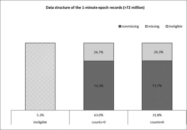
Accelerometer data structure and missingness

Among the records with positive counts, we identified 14 participants who had extremely large average counts while the average steps were very small. The observations from these participants were excluded from all the multiple imputation procedures because they should not have passed the data editing criteria for the NHANES.

3. Methods and models for multiply imputing the 2003-2004 NHANES steps data

For the missing steps with reported positive counts, we employed multiple imputation methods to impute the missing values. Due to missing data for entire PSUs, repeated measurements on individuals, and the skewness of the data as described earlier, finding the best model to impute the missing steps data was a difficult task. The development of the final imputation model involved several iterations. For a given model, we evaluated the imputation results using a simulation study that mimicked the actual missingness patterns. The evaluation results led to a modification of the model. The process was repeated several times until we found a final model that fit the data well. Features of the methods and final model will be described first, followed by a description of evaluations performed. A brief description of other models and methods considered will be given at the end of this section with further details given in the Appendix.

3.1 Multiple imputation based on Additive Regression, Bootstrapping and Predictive mean matching

Final multiple imputations were created using the ARBP approach, as implemented by the R package ‘‘aregImpute” [17]. Predictors used in the imputation models will be described first, followed by some details on the ARBP approach.

3.1.1 Predictors used in the imputation models

The imputation was done separately within the 12 groups formed by gender (male, female) and age categories (6-7, 8-11, 12-19, 20-39, 40-59, 60+) using a common set of predictor variables (see Table 1). We decided to run the imputation separately by those 12 groups because they are used to develop the sample weights, so it is recommended that when data analyses are stratified by gender and age groups that the strata used are these groups. Doing the imputation within these 12 groups also addresses the congeniality of the imputations. In addition, the relationships among the selected predictors and the response that were used in the imputation models varied across those groups.

Table 1.

List of covariates used for this study

Predictor variables	Type	Range of values or categories*
Counts1	continuous	1 to 32,703 (zeros were excluded)
Body Mass Index (kg/m2)	continuous	12.4 to 64.97
Standing height (cm)	continuous	109.6 to 203.2
Waist Circumference(cm)	continuous	32.0 to 170.7
Upper Leg Length (cm)2	continuous	24.7 to 54.0
Age at screener in months3	continuous	72 to 1,056
Day of the week	categorical	Monday, ..., Sunday.
Time of the day	categorical	‘Midnight-5:59am’, ‘6:00-11:59am’, ‘Noon-5:59pm’, ‘6:00-11:59pm’;
Race/Ethnicity4	categorical	Non-Hispanic White, Non-Hispanic Black, Mexican American, Other Race –Including Multi-Racial, and Other Hispanic
Full Sample 2Year MEC	continuous	1,673.6 to 159,302.8
Exam Sample Weight PSU	categorical	1,2, ..., 30 (30 PSUs)
Blood pressure(mm Hg) 2	continuous	79 to 227
Direct HDL-Cholesterol (mg/dL) 4	continuous	19 to 154
Education4	categorical	Less than high school, High school diploma (including GED), More than high school
Marital status4	categorical	Married vs Other
Smoking status4		Never smoker, current smoker, past smoker

¹Both minute level counts and person level average counts were included in the final imputation models.

²Upper leg length and blood pressure were included in the final imputation models for ages 8 years and older.

³Both age in months and square age in months were included in the final imputation models.

⁴HDL cholesterol, education, marital status, and smoking status were included in the final imputation models for ages 20+.

Counts was the most highly correlated predictor of steps. The Pearson correlation coefficient between steps and counts ranged from 0.62 to 0.81 across the 12 gender-age groups. Upper leg length was included as a predictor for the models of subjects 8 years old or older; it was not available for the 6-7 year olds. It is important to include sampling design information in multiple imputation for missing data with complex survey designs [18], therefore the sample weight and dummy variables indicating PSU were included as predictors to adjust for the complex sampling design. To account for person-level effects in steps, person level average counts was also included as a predictor. Given that the imputed data are typically provided to the data users for various analytic goals, a recommended practice is to include as many predictors as possible in the imputation model to ensure the imputation model is “congenial” with the models used for analyzing the multiple imputed data sets [12], even though some of these predictors may not be strongly associated with the outcome variable. Therefore, we also included race/ethnicity (for all age groups), blood pressure (for ages 8+), HDL cholesterol, education, marital status, and smoking status (for ages 20+) as predictors in the imputation models. Table A.1 in the Appendix reports the adjusted R-squares from the linear regression models of steps on the full list of covariates shown in Table 1 (call it the full model) and on square root of counts only (call it the reduced model). The similarity between the two sets of models indicates that the contribution of the covariates other than counts is negligible in predicting steps. Both age in months and square age in months were included in the final imputation models to adjust for person-specific age. The person level sample sizes for records that went into the linear regressions and multiple imputation procedures are also reported in Table A.1.

3.1.2 Imputation method using the ARBP approach

The ARBP approach was adopted to create the final multiple imputations. The ARBP approach fits ace models to estimate optimal transformations for both the predictors and the response variable (steps) used in the additive regressions.

A main feature of the ace algorithm is to provide nonlinear transformations of both the predictors and the response to maximize the correlation between the transformed response and the sum of the transformed predictors. An ace regression model has the general form:

$$g\left(Y\right)=\alpha +{\sum }_{j=1}^p{h}_j\left(x_j\right)+ϵ,$$

where g is a function of the response variable, Y,h_j are functions of the predictors x_j, j = 1, ..., p and ϵ is the error term. The optimal transformation functions g and h_j are estimated using an iterative method by minimizing $E\left\{{[g\left(Y\right)-{\sum }_{j=1}^p{h}_j\left(x_j\right)]}^2\right\}∕E{g}^2\left(Y\right)$, which involves unexplained variance, and maximizing the correlation between the transformed outcome and the sum of the transformed predictors. These optimal ace transformations are derived solely from the given data and do no require a priori assumptions of any functional form for the outcome or predictor variables and thus provide a powerful tool for exploratory data analysis. The a priori assumption-free feature of the ace algorithm also protects against uncongeniality.

The ARBP algorithm takes all aspects of uncertainty in the imputations into account by using the bootstrap to approximate the process of drawing predicted values from a full Bayesian predictive distribution. Instead of taking random draws of residuals from fitted imputation models, the algorithm by default uses predictive mean matching, where the observation having the closest predicted transformed value is the donor. To be more specific, after initialization and burn-in steps, the imputation algorithm is performed iteratively according to the following main steps: (1) for each variable containing any missing values, draw a sample with replacement from the observations in the entire dataset in which the current variable being imputed is non-missing; (2) fit a flexible additive model to predict this target variable while finding the optimum transformation of it (unless the identity transformation is forced); (3) use this fitted flexible model to predict the target variable in all of the original observations; and (4) impute each missing value of the target variable with the observed value whose predicted transformed value is closest to the predicted transformed value of the missing value following the predictive mean matching approach. Once the imputations are computed, the same process will be repeated to impute the next variable with missing values while including the imputed current variable as a predictor. The iterations repeat until all the variables with missing values are imputed. The whole imputation process is repeated multiple times to obtain multiply imputed data. For other options and more details, see [17]. For our data, we only have one target variable, steps, to be imputed.

Five sets of imputations for missing steps using ARBP approach were created for each of the 12 gender-age groups. Those 1-minute epoch records were combined with the 1-minute epoch records that went through logical imputation as well as those from the 14 participants that were excluded from the multiple imputation procedures. The final imputation file contains 68,527,007 eligible 1-minute epoch records where the accelerometer was in calibration (PAXCAL=1, where PAXCAL is a variable on the public use file indicating whether the accelerometer is in calibration) and the data were deemed reliable (PAXSTAT=1, where PAXSTAT is a variable on the public use file indicating reliability of the accelerometer data), with five sets of post imputation steps. We chose to use five imputations for practical reasons as the final imputation file is very large.

3.1.3 Imputation model evaluation through simulation

To evaluate the performance of the imputation method described in section 3.1.2, we conducted a simulation study using the observed data from the 22 PSUs with nearly complete data to check how well our imputation procedure using ARBP was working. To simulate a missing data pattern that was similar to the original missing data pattern, we randomly selected 6 out of the 22 PSUs (after removing the small number of the observations with missing steps), then set the observed steps in the selected PSUs to missing. We then applied the ARBP approach to produce 5 sets of multiply imputed data for the missing steps in the 6 PSUs using the observed data from the 16 remaining PSUs. The 1 minute epoch records with zero counts were excluded from this simulation study. Table A.2 at the appendix shows that the distribution of steps in the simulated data is similar to the original data.

We compared several statistics of the imputed values with those based on the original values for the 6 PSUs in the simulated data. The statistics included mean, standard deviation, median, mode, between person variance, within person variance and range (not weighted by the sample weights), which were used to describe the distribution of the original and imputed steps values for all the gender-age groups in the 6 PSUs from one of the sets of imputations (see Table S.1 in the Supplement file for details). We can see from the comparison that the distribution of the imputed data was similar to the distribution of the original data, except where the imputed data underestimate the between person component of variance. We repeated this simulation experiment 10 times by randomly resampling 6 PSUs to obtain relative biases. Similar results were found from all 10 experiments. Each experiment contained 12 independent ARBP MI programs for the 12 gender-age groups and the running time for each program varied from several hours to more than 10 hours using the NIH high-performance computing cluster system. There was also large overlap between the samples across experiments (simulations) because we randomly sampled 6 PSUs out of 22 PSUs for each simulation. We decided not to use more replications because of the similar results among the 10 experiments, the large computational burden for each experiment, and the large overlap among the samples across replication.

Let θ denote a summary statistic (e.g., mean, median) within a gender-age group, ${\theta }_i^{imp}$ and ${\theta }_i^{orig}$ denote the estimate based on imputed and original steps from the i-th simulation respectively. The relative bias of θ^imp (RELBIAS) was computed by averaging the relative differences between ${\theta }_i^{imp}$ and ${\theta }_i^{orig}$, i = 1, ..., m across the m experiments, i.e., $\mathrm{RELBIAS}=\frac{1}{m}{\sum }_{i=1}^m({\theta }_i^{imp}-{\theta }_i^{orig})∕{\theta }_i^{orig}$, where m=10 for our case. The corresponding standard Monte-Carlo simulation error for the relative bias of θ^imp (SE_RELBIAS) is computed as

$$\mathrm{SE}\_\mathrm{RELBIAS}=\sqrt{\frac{1}{m(m-1)}{\sum }_{i=1}^m{[({\theta }_i^{imp}-{\theta }_i^{orig})∕{\theta }_i^{orig}-\mathrm{RELBIAS}]}^2}.$$

Table 2 presents the relative biases and standard Monte-Carlo simulation errors of the statistics described earlier (those reported in Table S.1 in the supplement file). The imputations tended to slightly underestimate the various statistics given in Table S.1, with a large degree of underestimation for the between person component of variance. Table 3 presents the correlation coefficients between steps and counts using imputed and original steps, at the minute level and person level, as well as the averages of the within person correlation between steps (original and imputed) and counts. The relative biases in the correlation coefficients between the original and imputed data are reported in the same table, among which we can see some large relative biases. The results indicate that the imputed data generally preserved the minute level correlations, but increased the person level correlations even though we incorporated person level covariates as fixed effects in the models. Adding a person level random effect to the imputation model may be helpful to reduce the person level correlations. However, the current ARBP algorithm is not flexible enough to incorporate random effects. To add person level random effects to our imputation model, new algorithms based on mixed effect models [19] would have to be developed. Given the multiple levels of hierarchical data structure resulting from the complex multistage sample design and repeated measurements, and as mentioned earlier our goal of choosing an imputation approach that minimized model assumptions, we did not include a random effect component in our imputations. Practical concerns of the large data set size and the skewness of the data were also considerations for not including random effects.

Table 2.

Percent relative biases (and standard Monte Carlo simulation errors) of imputed steps based on ten sets of simulated data (using one set of imputed steps)^*

Gender	Age Group	Mean	Standard deviation	Median	Variance		Range
					Between person	Within person
Male	6-7	−0.22 (1.28)	−1.61 (1.55)	0.91 (1.63)	−13.21 (16.31)	−2.68 (2.97)	0.79 (1.64)
	8-11	−0.02 (0.61)	−1.03 (0.64)	0.39 (2.44)	−24.8 (5.95)	−1.31 (1.15)	−1.78 (0.94)
	12-19	−1.56 (0.65)	−1.56 (0.56)	−2.68 (2.78)	−22.85 (1.78)	−2.4 (1.1)	−0.91 (0.71)
	20-39	−1.8 (0.4)	−2.25 (0.57)	1.11 (1.11)	−31.58 (2.95)	−2.67 (1.17)	−3.68 (2.43)
	40-59	−0.37 (0.76)	−0.79 (0.78)	−2.08 (2.32)	−16.1 (3.12)	−0.75 (1.55)	1.19 (0.87)
	60+	−0.72 (0.53)	−0.95 (0.74)	4 (2.67)	−9.95 (3.69)	−1.35 (1.45)	−0.42 (2.33)
Female	6-7	−0.76 (1.22)	−1.54 (1.02)	1.17 (2.16)	−25.25 (13.05)	−2.3 (2.03)	−0.57 (1.92)
	8-11	−1.55 (0.59)	−2.22 (0.72)	−1 (1)	−10.3 (6.25)	−4.17 (1.44)	−2.56 (1.63)
	12-19	−0.56 (0.78)	−1.05 (0.84)	0 (0)	−27.06 (3.13)	−1.38 (1.72)	0.05 (1.45)
	20-39	−0.89 (0.78)	−0.53 (0.97)	−1.43 (1.43)	−38.51 (3.97)	0.33 (1.89)	5.93 (1.77)
	40-59	−0.58 (0.68)	−1.21 (0.58)	1.67 (2.7)	−33.24 (3.59)	−1.11 (1.12)	3.85 (2.59)
	60+	−0.09 (0.68)	−0.02 (0.83)	−4.67 (3.79)	−24.35 (2.49)	1.68 (1.68)	3.43 (4.38)

^*Notes: 1) Results were based on the 6 PSUs only. Records with zero counts were excluded from this simulation study.

2) Percentage relative bias was computed by averaging the ten percentage relative differences which were calculated by 100*(imputed-original)/original.

3) Mode was excluded from this table because of some zero modes in the denominator when calculated relative difference.

Table 3.

Correlation coefficients between steps and counts at both minute level and average person level (based on one set of imputed steps and one set simulated data), and average relative difference between imputed and original steps based on ten sets of simulated data

Gender	Age Group	CORR_m		CORR_P		CORR_Pave		Rel bias
		Original	imputed	Original	imputed	Original	imputed	CORR_m	CORR_P	CORR_Pave
Male	6-7	0.623	0.649	0.714	0.849	0.630	0.663	0.67 (1.29)	33.75 (16.1)	1.07 (1.00)
	8-11	0.678	0.674	0.718	0.734	0.708	0.703	0.03 (0.51)	20.76 (3.66)	−0.56 (0.52)
	12-19	0.771	0.770	0.774	0.939	0.791	0.795	−0.51 (0.37)	18.78 (0.9)	0.39 (0.42)
	20-39	0.838	0.809	0.866	0.905	0.847	0.822	−0.5 (0.62)	14.62 (1.4)	−0.11 (0.64)
	40-59	0.845	0.838	0.818	0.948	0.849	0.843	−0.61 (0.29)	18.53 (2.95)	−0.11 (0.32)
	60+	0.812	0.820	0.780	0.978	0.791	0.812	−0.46 (0.43)	15.86 (1.86)	3.28 (0.45)
Female	6-7	0.626	0.602	0.576	0.798	0.681	0.655	−0.29 (0.88)	31.37 (8.01)	−0.17 (0.94)
	8-11	0.691	0.672	0.631	0.801	0.720	0.700	−0.06 (0.81)	26.5 (4.76)	−0.71 (0.67)
	12-19	0.784	0.771	0.739	0.883	0.795	0.794	−0.1 (1.01)	39.07 (7.17)	1.73 (1.08)
	20-39	0.826	0.780	0.836	0.898	0.815	0.802	−0.37 (1.18)	35.06 (6.9)	1.57 (0.85)
	40-59	0.812	0.820	0.780	0.978	0.791	0.812	−1.61 (0.72)	20.98 (2.38)	0.31 (0.74)
	60+	0.794	0.784	0.860	0.961	0.741	0.774	0.1 (0.77)	13.18 (0.93)	6.32 (0.54)

CORR_m: The Pearson correlation between the minute level steps data (true and imputed) and the counts data.

CORR_P: The Pearson correlation between the person level average steps data (true and imputed) and the counts data.

CORR_Pave: The average of the within person correlation between the steps data (true and imputed) and the counts data.

Rel bias: Percentage relative bias, computed by averaging the ten percentage relative differences which were calculated by 100*(imputed-original)/original.

In Table 4 we present the between and within imputation variances as well as the ratio of the between to the total imputation variances for the mean steps (without using survey weights) based on one simulation experiment. We also present the average ratios based on the ten experiments. We can see that the between imputation variance ranges from about 2.5% to 36% of the total imputation variance indicating there can be a substantial contribution to the variability of estimates of mean steps due to the imputation process.

Table 4.

The between and within imputation variance for mean steps estimated from 5 sets of imputations

Gender	Age Group	Variance of mean steps based on one simulated data				Average ratio (between var over total var) based on five sets of simulated data
		Within imp	Between imp	Total	Between Var/Tot Var (%)	Average ratio (%)	Standard error (%)
Male	6-7	0.0016	0.0007	0.0025	29.6	27.3	3.8
	8-11	0.0009	0.0000	0.0009	5.2	20.4	7.4
	12-19	0.0003	0.0000	0.0003	10.4	10.0	3.6
	20-39	0.0003	0.0001	0.0004	15.9	10.6	2.2
	40-59	0.0001	0.0000	0.0001	11.6	16.0	2.5
	60+	0.0002	0.0001	0.0003	17.9	14.4	4.4
Female	6-7	0.0014	0.0004	0.0018	20.4	14.7	2.2
	8-11	0.0007	0.0001	0.0008	12.5	21.9	4.9
	12-19	0.0003	0.0000	0.0003	2.5	5.6	2.6
	20-39	0.0003	0.0001	0.0004	23.7	14.8	3.6
	40-59	0.0002	0.0001	0.0003	18.4	15.8	4.0
	60+	0.0001	0.0000	0.0001	35.6	28.8	3.9

As a further empirical examination of the imputation methods, we compared the covariates for the observations with missing steps to those without missing steps to help explain differences between the imputed and original steps. Using two sample t-tests we compared the gender-age group means between those individuals with missing steps to those with observed steps for the continuous covariates (except counts) listed in Table 1. We found no significant differences for the majority of the comparisons except those for the 20-39 year old male group.

3.2 Other multiple imputation models considered

Before deciding on the ARBP method we considered a wide range of methods involving multiple imputation. This section provides a short summary of our efforts; see Figure 2 for a flowchart of the methods we investigated and the Appendix for more details. Given the fact that the steps and counts data are both continuous and highly correlated, we initially tried to adopt multiple linear regression multiple imputation approaches to address the missing steps data from affected accelerometers in the 2003-2004 NHANES. These models involved regressing steps on counts, square root of counts, and 3, 4 and 5 knot restricted cubic regression splines of counts. Because the predicted steps from these regression models could be out of range, we considered linear regression models with various constraints on the range of the predicted steps. Box-Cox transformation of steps was also considered. Next propensity score imputation and propensity scores included as covariates in a multiple linear regression imputation model, predictive mean matching, and a benchmarking approach in conjunction with the square root transformed counts in a multiple linear regression model were considered. In general we were unable to remove imputation bias that was detected from the simulation evalution, especially bias in the median, mode and within and between person variances of steps. These multiple imputations were implemented using the PROC MI procedure in SAS 9.3 (SAS Institute Inc., Cary, NC), a general program that performs multiple imputations with regression models and an approximate Bayesian bootstrap [13] or Monte Carlo Markov Chain approach. We used the standard PROC MI syntax that is available from the SAS online manual (https://support.sas.com/documentation/cdl/en/statug/63033/HTML/default/viewer.htm#statug_ mi_sect003.htm). Per one reviewer's suggestion, we include the core PROC MI codes for the group of 6-7 year old boys at Appendix A.3. The PROC MI code for the rest of the gender-age groups are the same as the 6-7 year old boys except for a few additional predictors that were applicable only for certain age groups as described in Table 1. Other parts of the codes are available upon request to the authors.

Figure 2.

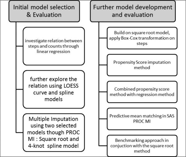
Flowchart of other imputation models considered

4. Analyses of multiply imputed steps data from the 2003-2004 NHANES

This section illustrates properties of the multiply imputed steps through typical analyses of accelerometer data found in the literature. Estimates of population quantities and estimated standard errors are compared between analyses with multiply imputed data and those obtained with complete cases. We used SAS 9.3 sample survey procedures to account for the complex sampling design of NHANES. We followed the method of analyzing multiply imputed data given in section 3.3-3.5 of Rubin's book [13] and used SAS PROC MIANALYZE (http://support.sas.com/rnd/app/stat/procedures/mianalyze.html) to obtain the final estimates and standard errors based on the five sets of final multiply imputed data.

4.1 Analyses of the patterns of stepping cadence in the 2003-2004 NHANES

Cadence (steps per minute) is a gait parameter that has been traditionally measured using short distance walking tests. Laboratory studies of adult walking behavior have consistently found that a cadence of 100 steps/min is a reasonable threshold for moderate intensity. Several papers in the literature analyzed the patterns of adult or youth stepping cadence and peak stepping cadence in the 2005-2006 NHANES (e.g., [4]-[6]). Cadence has been used to describe step accumulation patterns as a way to study free-living ambulatory behavior. We repeated some of the cited analyses on stepping cadence using the 2003-2004 NHANES data with and without imputing the missing steps.

Data collected by accelerometers such as Actigraph in a natural free-living environment can be divided into wear and nonwear time intervals. Nonwear time intervals include periods during which participants are asked not to wear their monitor, such as sleeping, showering, and aquatic activities. Wear time usually includes all waking periods and requires a specific number of hours of wearing for a day to be considered valid [20]. For this study, a SAS macro (http://riskfactor.cancer.gov/tools/nhanes_pam/) supplied by the National Cancer Institute was used to determine nonwear time (defined as >=60 consecutive zeros, allowing minimal interruptions). To be consistent with the literature, a valid day was defined as having at least 10 hours of accelerometer wear time on a day and the analyses were limited to those participants with at least one valid day of data.

At the 1-minute epoch record file (with and without imputing the missing steps), we first defined the cadence variable from steps using the zero category and seven categories of approximately 20-step-per-minute increments: zero cadence (non-movement during wearing time), 1-19 (incidental movement), 20-39 (sporadic movement), 40-59 (purposeful steps), 60-79 (slow walking), 80-99 (medium walking), 100-119 (brisk walking), and 120+ (faster locomotion) steps per minute. Then within each nonzero cadence category, the average amount of time (min/day) and average steps/day were calculated over valid days for each participant. Finally within each age-gender group, the overall average amount of time (min/day) and overall average steps/day accounting for the survey weights and sample design were computed within each cadence category. The computation was repeated twice, with and without imputed steps. The time spent at zero steps per minute (excluding nonwear time) was also calculated. Figure 3 shows the scatter plots of the estimated mean minutes/day accumulated within each designated incremental cadence category (including minutes of zero cadence) recorded during wearing time for the overall sample and the 12 gender-age groups before and after imputation. Figure 4 shows the scatter plots of the estimated mean steps/day under the same structure. Note that the scales in Figures 3 and 4 differ across the different cadence categories to present the spread of the data points better than possible with a common scale. The detailed numerical results are presented in Tables S.2 and S.3 in the supplement file. From Figures 3 and 4, we can see that for both steps/day and minutes/day, the estimated means are very similar before and after imputation except for the fastest locomotion cadence category (steps/min ≥120) where the means of the pre-imputed data are larger than the means after imputation. We explored further for the fastest locomotion cadence category using the simulated data and found similar patterns (see Figure 5). This indicates that the imputation method may introduce some bias for extreme steps. From the standard errors shown in Tables S.2 and S.3 in the supplemental file, we can see that the estimated means after imputation compared to those before imputation have smaller standard errors for about 2/3 of the estimates, indicating the imputation is conferring increased efficiency.

Figure 3.

Scatter plots of the estimated mean minutes/day accumulated within each designated incremental cadence category (including minutes of zero cadence) recorded during wearing time for the overall sample and the 12 gender-age groups based on steps before and after imputation

Figure 4.

Scatter plots of the estimated mean steps/day accumulated within each designated incremental cadence category recorded during wearing time for the overall sample and the 12 gender-age groups based on steps before and after imputation

Figure 5.

Scatter plot of the estimated mean minutes/day and steps/day for the Faster Locomotion cadence category for the overall sample and the 12 gender-age groups based on steps before and after imputation – from one simulated data

4.2 Analyses of the relationship between accelerometer-determined steps/day and metabolic syndrome

Sisson et al [7] analyzed the associations between accelerometer-determined steps/day and the odds of having metabolic syndrome (MetS) and its individual cardiovascular disease (CVD) risk factors in the U.S. population using the 2005-2006 NHANES data. We repeated part of their regression analyses using the 2003-2004 NHANES data with some minor modifications. The same process as described in Section 4.1 was used to determine the valid days and valid participants aged 20+.

Following the American Heart Association/National Heart, Lung, and Blood Institute (AHA/NHBLI) guidelines [21], classifications of MetS were based on three or more of the following: 1) high waist circumference (>=102 cm for men and >=88 cm for women); 2) high levels of triglycerides (>=150 mg/dL or on drug treatment); 3) low level of HDL cholesterol (<40 mg/dL for men and <50 mg/dL in women or on drug treatment); 4) elevated blood pressure (>=130 mmHg systolic or >=85 mmHg diastolic or drug treatment); 5) elevated fasting glucose (>=100 mg/dL or on drug treatment).

Logistic regression models were used to determine if steps/day was associated with odds of MetS and individual CVD risk factors. The associations of the continuous steps/day with the prevalence of MetS and the individual CVD risk factors were investigated for the total sample, and separately for men and women, adjusting for age, gender, ethnicity (NH white, NH Black, Mexican American, other), education (<high school, high school degree or equivalent, > high school), percentage fat in diet, and usual occupational/domestic physical activity (sits mostly vs stands/carries loads/heavy work). The analyses were repeated two times, once using steps without imputation, and the other using the five sets of multiply imputed steps.

Odds ratios for the continuous steps/day (per 1000 steps/day) for predicting metabolic syndrome and the five individual CVD risk factors with and without imputation for steps were computed (see Table S.4 in the supplement file). The results are generally consistent before and after imputation. A reviewer noted that it is not surprising to see the similarity between before and after imputation for the odd ratios for metabolic syndrome as a function of steps since there is little information about the bivariate relationship given that the steps were imputed. Information recovery could be larger for other parameters.

We also fitted the models without adjusting for usual occupational/domestic physical activity. The odds ratios for steps/day were very similar to those reported in Table S.4, so we do not report them in this paper.

5. Summary and Discussion

This paper describes the statistical methodology and procedures used to impute missing steps data from incorrectly initialized accelerometers in the NHANES 2003-2004. Due to the special missingness situation (repeated measurements within person, missing a variable for all persons within a PSU) and skewness of this data set, various commonly used imputation methods did not work well for the missing steps data. After trying several approaches including propensity score, linear regression, linear regression with transformations (e.g., square root transformation of the counts data, Box-Cox transformations of the steps data) and spline model regression, which either did not preserve relationships between variables (the propensity score method) or showed consistent imputation biases resulting in higher means, medians and modes, a semiparametric multiple imputation approach, ARBP, based on ace models and predictive mean matching was adopted, The imputation using ARBP was applied separately for each of the 12 gender-age groups. Several approaches were used for data analyses and model diagnostics (as suggested in [22]). We also compared the distribution of the observed data with the distribution of the imputed data in an experiment that simulated the missingness patterns in order to better understand how well the imputed data reflected the distribution of the original data. The different analyses and evaluations showed that the imputation using ARBP worked fairly well except that it may have some limitations on imputing extreme steps.

Generally, using imputed data has the potential to adjust for biases that can occur with complete-case analysis and other methods by incorporating predictors observed for both complete and incomplete cases in the imputation model; and using multiple imputations reflects the extra uncertainty due to imputation. Although there was not clear evidence of such biases in our analyses regardless of the unusual mechanism of missingness, there was greater efficiency from the imputation by utilizing data on counts and other variables from the PSUs with missing steps data in the imputation models.

A goal of this study was to make the final imputed steps data publicly available so that researchers can utilize them for their particular data analyses. Since the missing data were mainly isolated in certain PSUs that convey geographical information, the flagging of the imputed data along with other information in the NHANES could reveal the identity of surveyed individuals. To protect confidentiality and for ease in data analysis, we considered releasing just one single set of imputed data without flagging. However, based on our five sets of imputed data, we found that the between imputation variances were nontrivial and should not be ignored. An alternative option would be to make multiple sets of imputed data available through a research data center because of the potential disclosure risk involved.

Recent research (e.g., [23]) has suggested use of greater than the traditional number of five or fewer sets of imputed data, especially if the fractions of missing information for various analyses are high. Thus, if multiply imputed data for steps in the 2003-2004 NHANES are made available, a larger number of imputations could be considered, though the large size of the imputed data set would need to be taken into account. Creation of additional sets of imputations is straightforward once the imputation model has been developed, and the handling of larger numbers of imputations in standard analyses is facilitated through the use of software packages that include programs for analyzing multiply imputed data. For specialized analyses, especially those that require human intervention during the analysis, however, using a small number of imputations is desirable. With one of the simulated data, we compared the between imputation variance using 20 sets versus five sets of multiply imputed data and found no difference. Given the computational resource requirements for analyzing these data, we feel five sets are sufficient.

Appendix

Appendix A: Other multiple imputation models considerred

A.1 Initial model selection and evaluation

We started with investigating the relationship between steps and counts. We ran a regression model on steps including a linear term for counts as the predictor. The range of the predicted steps based on the linear model relationship was much wider than the range of the observed steps (400+ compared to 200). We also examined scatter plots of steps against counts. For example, the scatter plot for the 6-7 year old boys is given in Figure A.1. The nonlinear shape of the scatter plot suggested that a square root transformation of intensity may improve the linear relationship between steps and counts. The estimated Pearson correlation coefficients between steps and counts across the 12 gender-age groups increased from 0.62-0.81 (before the square root transformation) to 0.75-0.86 (after the square root transformation), indicating a stronger linear relationship between steps and the square root of counts. A logrithmic transformation was also considered but then dropped because the square root transformation showed a larger correlation with the steps variable.

Figure A.1.

Scatter plot of steps against counts with default LOESS fit for 6-7 year old boys

To further explore the relationship between steps and counts, we fitted a LOESS curve through the scatter plot (see the grey line in Figure A.1). The nonlinear shape of the LOESS curve suggested using a restricted cubic regression spline for counts in the prediction model [24]. We therefore considered 3, 4 and 5 knot splines of the counts variable and compared prediction of steps from these three spline models to the prediction of steps from the regression model with counts as a linear variable and the regression model with the square root of counts. All five regression models included the other covariates listed in Table 1 as well. The box-plots of the observed steps and the predicted steps for each gender-age group from the five regression models were examined (plots not shown). The predicted steps using the square root transformation appeared to reflect the range and extreme percentiles of the observed steps better than the other models. However, when using a spline, the adjusted R-squares were larger, the residual plots appeared to be more symmetric (data not shown) and the median and interquartile range of the predicted steps values were somewhat closer to the observed steps data than for the model using the square root transformation. The performance of the three spline models were very similar, with slightly better performance from the 4 knot spline. Based on this analysis, we dropped the linear model and the models with the 3 or 5 knot splines from further analysis.

To evaluate the two sets of competitive regression models, using either a square root transformation or a 4-knot spline of the counts variable, we used the same simulated data as those described in Section 3.1.3. We applied SAS PROC MI, using the multiple linear regression method. To limit the range of imputed steps, we set constraints of maximum=200 and minimum=0. PROC MI uses a proper imputation methodology where the procedure fits the regression model first based on the observed data. For each imputation, new parameter values are drawn from the posterior predictive distribution of the parameters [9]. If the constraints are not satisfied, the procedure randomly redraws the parameters until the constraints are satisfied or the pre-defined maximum number of iterations is reached. For more details about this procedure, see http://support.sas.com/rnd/app/papers/miv802.pdf.

We compared the imputed steps from each model with the original steps using the simulation approach described in Section 3.1.3, where 6 randomly selected PSUs with complete steps and counts data were set to have missing steps data. We found that the imputed data had a higher median and mean than the original value. Similar results were found from all 10 experiments (data not shown), which indicated that the two linear models selected may introduce imputation bias.

A.2 Further model development and evaluation

Since the model evaluation in section 3.2.1 indicated some imputation bias in the two models identified (using the 4-knot spline or square root transformed counts), we explored other imputation approaches based on linear regression. We discarded the 4-knot spline model since it violated the maximum=200 constraint for three of the gender-age groups and produced no better results than the square root model. The following summarizes the various imputations approaches and findings.

Starting with the imputation model with square root transformed counts (call it square root model from now on), we applied the Box-Cox transformation [25] to the dependent variable (steps) and examined its performance using the same simulation data as described earlier. The evaluation results showed that using a Box-Cox transformation helped to reduce bias for only some of the gender-age groups (e.g., female 12-19, female 20-39). However, the maximum limit restriction had to be relaxed for most of the gender-age groups in order to make the program run successfully, which resulted in some extreme imputed values (e.g., steps>=600) that had to be truncated.

Next we considered a propensity score imputation method implemented in SAS PROC MI (http://support.sas.com/documentation/cdl/en/statug/63033/HTML/default/viewer.htm#statug_mi_sect021.htm). For each gender-age group, this procedure first creates an indicator variable with value zero for observations with missing steps and value one otherwise, and then fits a logistic regression model (using the same covariates as those included in the square root model) to create propensity scores. The observations within each gender-age group were then divided into a fixed number of groups (we used three for the 6-7 year old and five for all other gender-age groups) based on the propensity scores. Finally an approximate Bayesian bootstrap imputation [11] was applied to each propensity group [26]. The same procedure was repeated multiple times to form multiple imputation sets. The model diagnostics using the simulated data showed that the propensity score approach maintained the marginal distributions, but not the correlation between the steps and counts. For example, the person correlation between the steps and counts for the 6-7 years old reduced from 0.6233 based on original data to 0.0018 based on imputed data. Similar reduction were found in most other gender-age groups (data not shown).

We also combined a propensity score method with the regression method. Within each gender-age group, five approximately equally sized categories of observations (three for the 6-7 year old) were formed with similar propensities before we applied the square root modeling approach within each gender-age-propensity category. The evaluation results using simulated data did not show any improvement using this approach in terms of reduction in imputation bias.

We next tried to use the predictive mean matching method of imputation implemented in SAS PROC MI (http://support.sas.com/documentation/cdl/en/statug/63033/HTML/default/viewer.htm#statug_mi_sect020.htm). The predictive mean matching method ensures that imputed values are plausible and might be more appropriate than the regression method if the normality assumption is violated [27]. However, due to the large database, the computations were not feasible.

Finally we used a benchmarking approach in conjunction with the square root regression model method with the following 3 steps: (1) do multiple imputation (five times) for minute level steps using the square root model through PROC MI; (2) do multiple imputation (also five times) for person level average steps through a corresponding person level square root model, using person level average for steps and the square root of counts (the records included in the model are at person level); and (3) benchmark the minute level imputed steps to the person level imputed steps so that the aggregated mean steps from the minute level imputation match with the person level imputed steps. For each imputation set, the calibration was carried out only once instead of five times using randomly assigned unique pairs. The evaluation results using simulated data showed a slight reduction in the imputation bias compared to the square root model approach.

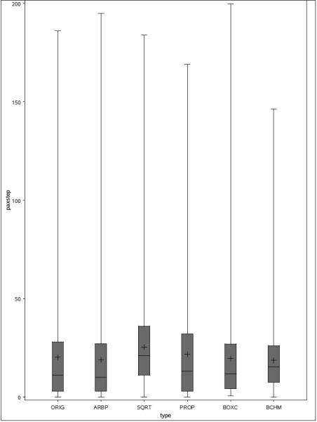
Figure A.2 displays overview box-plots of the original steps and the predicted steps for the 6-7 years old boys from five different multiple imputation methods for the 6 PSUs from one simulation (only one set of the multiply imputed data was used): the ARBP approach (ARBP), the square root model (SQRT), the propensity score approach (PROP), the Box-Cox transformed model (BOXC), and the benchmarking approach (BCHM). An extreme imputed value produced by the Box-Cox transformed method (imputed steps >600) was removed from the plot for a better comparison across the different methods. Overall, the ARBP approach performed the best among all the methods we considered across all the age-gender groups.

Figure A.2.

Box-plot of the original and imputed steps for 6-7 years old boys for 6 NHANES PSUs randomly selected with participants with both steps and counts data.

A.3 SAS codes for PROC MI

/*paxstep is the variable name for steps*/
/*paxinten is the varaible name for counts*/
/*paxinten2 is the square root of counts*/
/*paxinten_p is the person level average of counts*/
/* SPL4INTEN1 and SPL4INTEN2 are the knots variables created for splines with 4 knots*/
/* paxstep_boxcox is the boxcox transformed steps variable*/
/*“bmxbmi paxday timea bmxht bmxwaist agemon agemonsq wtmec2yr ridreth2 PSU” are the rest predictor names used for the 6-7 year olds, see Table 1 for details*/

PROC MI codes for the square root model

proc mi data=inputfilename seed=13951639 minimum=0 maximum=200 NIMPUTE=5 MINMAXITER=1000000 round=1
out=outputfilename(keep=seqn paxn riagendr agea paxstep_orig paxstep_missstat2 paxstep_noimp _imputation_ paxstep paxinten paxinten_p);
class paxday timea ridreth2 PSU;
var paxinten2 paxinten_p bmxbmi paxday timea bmxht bmxwaist agemon agemonsq wtmec2yr ridreth2 PSU paxstep;
monotone reg(paxstep = paxinten2 paxinten_p bmxbmi paxday timea bmxht bmxwaist agemon agemonsq wtmec2yr ridreth2 PSU/ details); run;

PROC MI codes for the 4 spline model

proc mi data= inputfilename seed=13951639 minimum=0 maximum=200 NIMPUTE=5 MINMAXITER=1000000 round=1
out= outputfilename (keep=seqn paxn riagendr agea paxstep_orig paxstep_missstat2 paxstep_noimp _imputation_ paxstep paxinten paxinten_p);
class paxday timea ridreth2 PSU;
var paxinten SPL4INTEN1 SPL4INTEN2 paxinten_p bmxbmi paxday timea bmxht bmxwaist agemon agemonsq wtmec2yr ridreth2 PSU paxstep;
monotone reg(paxstep = paxinten SPL4INTEN1 SPL4INTEN2 paxinten_p bmxbmi paxday timea bmxht bmxwaist agemon agemonsq wtmec2yr ridreth2 PSU/details); run;

PROC MI codes for the Boxcox model

proc mi data= inputfilename seed=13951639 minimum=0.717734625 maximum=9 NIMPUTE=5 MINMAXITER=1000000 round=1
out= outputfilename (keep=seqn paxn riagendr agea paxstep_orig paxstep_missstat2 paxstep_noimp _imputation_ paxstep_boxcox paxinten paxinten_p);
class paxday timea ridreth2 PSU;
var paxinten2 paxinten_p bmxbmi paxday timea bmxht bmxwaist agemon agemonsq wtmec2yr ridreth2 PSU paxstep_boxcox;
monotone reg(paxstep_boxcox = paxinten2 paxinten_p bmxbmi paxday timea bmxht bmxwaist agemon agemonsq wtmec2yr ridreth2 PSU/ details); run;

PROC MI codes for the propensity model

proc mi data= inputfilename seed=13951639 NIMPUTE=5 MINMAXITER=1000000 round=1
out= outputfilename (keep=seqn paxn riagendr agea paxstep_orig paxstep_missstat2 paxstep_noimp _imputation_ paxstep paxinten paxinten_p);
class paxday timea ridreth2 PSU;
var paxinten2 paxinten_p bmxbmi paxday timea bmxht bmxwaist agemon agemonsq wtmec2yr ridreth2 PSU paxstep;
monotone propensity(paxstep = paxinten2 paxinten_p bmxbmi paxday timea bmxht bmxwaist agemon agemonsq wtmec2yr ridreth2 PSU/ NGROUPS=3 details); run;

PROC MI codes for the PMM model

proc mi data= inputfilename seed=13951639 minimum=0 maximum=200 NIMPUTE=5 MINMAXITER=1000000 round=1
out= outputfilename (keep=seqn paxn riagendr agea paxstep_orig paxstep_missstat2 paxstep_noimp _imputation_ paxstep paxinten paxinten_p);
class paxday timea ridreth2 PSU;
var paxinten2 paxinten_p bmxbmi paxday timea bmxht bmxwaist agemon agemonsq wtmec2yr ridreth2 PSU paxstep;
monotone regpmm(paxstep = paxinten2 paxinten_p bmxbmi paxday timea bmxht bmxwaist agemon agemonsq wtmec2yr ridreth2 PSU/ details); run;

Appendix B: Appendix tables for Section 3

Table A.1.

Person level sample sizes^* and adjusted R-squares from the minute level linear regressions of steps on the full list of predictors (full model) and on square root of counts only (the reduced model)^**

Gender	Age	total number of respondents	number of respondents with nonmissing steps	Adjusted R2 from Full model	Adjusted R2 from Reduced model
Male	6-7	136	99	0.5633	0.5602
	8-11	268	196	0.6334	0.6276
	12-19	978	712	0.7484	0.7406
	20-39	643	474	0.7559	0.7524
	40-59	572	433	0.7691	0.7572
	60+	729	528	0.7116	0.7021
Female	6-7	145	113	0.5623	0.5576
	8-11	299	238	0.6145	0.6145
	12-19	916	665	0.705	0.6982
	20-39	756	546	0.6861	0.6836
	40-59	608	442	0.6979	0.6818
	60+	749	541	0.6459	0.6378

^*The sample sizes are for the person level records that went into the linear regressions and the multiple imputation procedures.

^**The models were run with minute level records.

Table A.2.

Distribution of steps in the original (full set) data and in one set of simulated data (complete case analysis)

Gender	AGEGROUP	Mean		STD		Median		Mode		Between Person Variance		Within Person Variance		Range
		Original	Sim	Original	Sim	Original	Sim	Original	Sim	Original	Sim	Original	Sim	Original	Sim
Male	6-7	20.4	20.5	24.2	24.3	11	11	1	1	13.2	13.1	573.8	578.1	196	196
	8-11	18.9	18.9	24.2	24.1	9	9	1	1	14.4	14.9	570.9	567.1	199	199
	12-19	18.5	18.0	25.6	25.2	7	7	1	1	21.5	19.8	632.0	613.0	198	198
	20-39	18.3	18.3	22.8	22.4	9	10	1	1	29.2	29.7	491.0	472.1	208	188
	40-59	17.1	17.2	21.8	21.8	9	9	0	0	24.0	24.7	453.0	448.6	178	178
	60+	13.3	13.2	19.2	19.2	6	6	0	0	22.9	26.8	346.5	340.3	182	176
Female	6-7	19.3	19.4	23.2	23.2	11	11	1	1	10.1	10.7	528.7	529.2	195	194
	8-11	18.0	18.2	23.2	23.2	9	9	1	1	9.9	10.3	530.0	530.1	197	193
	12-19	16.2	16.1	24.0	23.7	6	6	1	1	14.6	15.3	563.3	546.2	199	199
	20-39	15.1	14.8	20.7	20.3	7	7	1	0	14.5	18.8	412.2	391.5	195	195
	40-59	14.5	14.1	20.0	19.7	7	6	1	0	17.4	22.5	381.0	364.7	185	185
	60+	11.7	11.6	17.2	17.2	5	5	0	0	18.6	17.8	278.4	276.5	172	172

References

- 1.NCHS. National Health and Nutrition Examination Survey, Laboratory Procedures Manual. National Center for Health Statistics; Hyattsville, MD: Jan, 2004. Chapter 16 ( https://www.cdc.gov/nchs/data/nhanes/nhanes_03_04/lab.pdf) [Google Scholar]
- 2.Troiano RP, Berrigan D, Dodd KW, Masse LC, Tilert T, McDowell M. Physical activity in the United States measured by accelerometer. Med Sci Sports Exerc. 2008;40(1):181–188. doi: 10.1249/mss.0b013e31815a51b3. [DOI] [PubMed] [Google Scholar]
- 3.Matthews CE, Chen KY, Freedson PS, Buchowski MS, Beech BM, Pate RR, Troiano RP. Amount of time spent in sedentary behaviors in the United States, 2003-2004. Am J Epidemiol. 2008;167(7):875–881. doi: 10.1093/aje/kwm390. [DOI] [PMC free article] [PubMed] [Google Scholar]
- 4.Tudor-Locke C, Camhi SM, Leonardi C, Johnson WD, Katzmarzyk PT, Earnest CP, Church TS. Patterns of adults stepping cadence in the 2005-2006 NHANES. Preventive Medicine. 2011;53(3):178–181. doi: 10.1016/j.ypmed.2011.06.004. [DOI] [PubMed] [Google Scholar]
- 5.Tudor-Locke C, Brashear MM, Katzmarzyk PT, Johnson WD. Peak stepping cadence in free-living adults: NHANES 2005-2006. J Phys Act Health. 2012;9(8):1125–1129. doi: 10.1123/jpah.9.8.1125. [DOI] [PubMed] [Google Scholar]
- 6.Barreira TV, Katzmarzyk PT, Johnson WD, Tudor-Locke C. Cadence patterns and peak cadence in US Children and adolescents: NHANES, 2005-2006. Med Sci Sports Exerc. 2012;44(9):1721–1727. doi: 10.1249/MSS.0b013e318254f2a3. [DOI] [PubMed] [Google Scholar]
- 7.Sisson SB, Camhi SM, Church TS, Turdor-Locke C, Johnson WD, Katzmarzyk PT. Accelerometer-determined steps/day and metabolic syndrome. Am J Prev Med. 2010;38(6):575–582. doi: 10.1016/j.amepre.2010.02.015. [DOI] [PubMed] [Google Scholar]
- 8.Tudor-Locke C, Johnson WD, Katzmarzyk PT. Relationship Between Accelerometer-Determined Steps/Day and Other Accelerometer Outputs in U.S. Adults. J Phys Act Health. 2011;8(3):410–419. doi: 10.1123/jpah.8.3.410. [DOI] [PubMed] [Google Scholar]
- 9.Little RJA, Rubin DB. Statistical Analysis with Missing Data. Wiley; New York: 2002. [Google Scholar]
- 10.Schafer JL, Graham JW. Missing data: Our view of the state of the art. Psychological Methods. 2002;7(2):147–177. [PubMed] [Google Scholar]
- 11.Rubin DB. Multiple Imputation for Nonresponse in Surveys. Wiley; New York: 1987. [Google Scholar]
- 12.Meng X-L. Multiple Imputation Inferences with Uncongenial Sources of Input. Statistical Science. 1994;9:538–573. [Google Scholar]
- 13.Catellier DJ, Hannan PJ, Murray DM, Addy CL, Conway TL, Yang S, Rice JC. Imputation of missing data when measuring physical activity by accelerometry. Med Sci Sports Exerc. 2005;37(11 Suppl):S555–562. doi: 10.1249/01.mss.0000185651.59486.4e. [DOI] [PMC free article] [PubMed] [Google Scholar]
- 14.Lee PH. Data imputation for accelerometer-measured physical activity: the combined approach. Am J Clin Nutr. 2013;97(5):965–971. doi: 10.3945/ajcn.112.052738. [DOI] [PubMed] [Google Scholar]
- 15.Kang M, Rowe DA, Barreira TV, Robinson TS, Mahar MT. Individual information-centered approach for handling physical activity missing data. Res Q Exerc Sport. 2009;80(2):131–137. doi: 10.1080/02701367.2009.10599546. [DOI] [PubMed] [Google Scholar]
- 16.Breiman L, Friedman JH. Estimating Optimal Transformations for Multiple Regression and Correlation. Journal of the American Statistical Association. 1985;80(391):614–619. [Google Scholar]
- 17.Harrell FE., Jr Package “Hmisc”. 2016 ( http://cran.r-project.org/web/packages/Hmisc/Hmisc.pdf)
- 18.Reiter JP, Raghunathan TE, Kinney SK. The Importance of Modeling the Sampling Design in Multiple Imputation for Missing Data. Survey Methodology. 2006;32(2):143–149. [Google Scholar]
- 19.McCulloch CE, Searle SR, Neuhaus JM. Generalized, Linear, and mixed Models. 2ndEdition John Wiley & Sons, Inc.; 2008. [Google Scholar]
- 20.Choi L, Liu Z, Matthews CE, Buchowski MS. Validation of Accelerometer Wear and Nonwear Time Classification Algorithm. Med Sci Sports Exerc. 2011;43(2):357–364. doi: 10.1249/MSS.0b013e3181ed61a3. [DOI] [PMC free article] [PubMed] [Google Scholar]
- 21.Grundy SM, Cleeman JI, Daniels SR, Donato KA, Eckel RH, Franklin BA, Gordon DJ, Krauss RM, Savage PJ, Smith SC, Jr, Spertus JA, Costa F. Diagnosis and management of the metabolic syndrome: an American Heart Association/National Heart, Lung, and Blood Institute scientific statement: executive summary. Circulation. 2005;112(17):2735–2752. doi: 10.1161/CIRCULATIONAHA.105.169404. [DOI] [PubMed] [Google Scholar]
- 22.Abayomi K, Gelman A, Levy M. Diagnostics for multivariate imputations. Journal of the Royal Statistical Society. Series C (Appl. Statist.) 2008;57:273–291. [Google Scholar]
- 23.Graham JW, Olchowski AE, Gilreath TD. How many imputations are really needed? Some practical clarifications of multiple imputation theory. Prevention Science. 2007;8:206–213. doi: 10.1007/s11121-007-0070-9. [DOI] [PubMed] [Google Scholar]
- 24.Durrleman S, Simon R. Flexible regression models with cubic splines. Statistics in Medicine. 1989;8(5):551–61. doi: 10.1002/sim.4780080504. [DOI] [PubMed] [Google Scholar]
- 25.Box GEP, Cox DR. An analysis of transformations. Journal of the Royal Statistical Society. Series B (Methodological) 1964;26(2):211–252. [Google Scholar]
- 26.Lavori P, Dawson R, Shera D. A multiple imputation strategy for clinical trials with truncation of patient data. Statistics in Medicine. 1995;14:1912–1925. doi: 10.1002/sim.4780141707. [DOI] [PubMed] [Google Scholar]
- 27.Horton NJ, Lipsitz SR. Multiple Imputation in Practice: Comparison of Software Packages for Regression Models With Missing Variables. The American Statistician. 2001;55:244–254. [Google Scholar]
Associated Data
This section collects any data citations, data availability statements, or supplementary materials included in this article.