Abstract
Diffusion magnetic resonance imaging (dMRI) can be used for noninvasive imaging of white matter tracts. Using fiber tracking, which propagates fiber streamlines according to fiber orientations (FOs) computed from dMRI, white matter tracts can be reconstructed for investigation of brain diseases and the brain connectome. Because of image noise, probabilistic tractography has been proposed to characterize uncertainties in FO estimation. Bootstrap provides a nonparametric approach to the estimation of FO uncertainties and residual bootstrap has been used for developing probabilistic tractography. However, recently developed models have incorporated sparsity regularization to reduce the required number of gradient directions to resolve crossing FOs, and the residual bootstrap used in previous methods is not applicable to these models. In this work, we propose a probabilistic tractography algorithm named Lasso bootstrap tractography (LBT) for the models that incorporate sparsity. Using a fixed tensor basis and a sparsity assumption, diffusion signals are modeled using a Lasso formulation. With the residuals from the Lasso model, a distribution of diffusion signals is obtained according to a modified Lasso bootstrap strategy. FOs are then estimated from the synthesized diffusion signals by an algorithm that improves FO estimation by enforcing spatial consistency of FOs. Finally, streamlining fiber tracking is performed with the computed FOs. The LBT algorithm was evaluated on simulated and real dMRI data both qualitatively and quantitatively. Results demonstrate that LBT outperforms state-of-the-art algorithms.
Keywords: Diffusion magnetic resonance imaging, probabilistic tractography, Lasso bootstrap
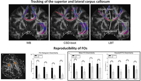
Graphical Abstract
1. Introduction
Diffusion magnetic resonance imaging (dMRI) is currently the only tool for in vivo investigation of white matter tracts. It captures the anisotropy of water diffusion in tissue to extract information about fiber tract orientations, which enables the reconstruction of white matter tracts (Johansen-Berg and Behrens, 2013). Diffusion tensor imaging (DTI) was first invented to model the water diffusion using a Gaussian distribution (Basser et al., 1994). Due to the inability of DTI to model crossing fiber tracts, more advanced dMRI techniques, such as high angular resolution diffusion imaging (HARDI) (Tuch et al., 2002) and diffusion spectrum imaging (DSI) (Wedeen et al., 2005), have been developed.
Using dMRI, fiber tracking—also known as tractography—can be performed to reconstruct white matter tracts (Mori et al., 2005). It has been used to investigate pathological abnormalities of specific tracts in a variety of diseases such as multiple sclerosis (Vishwas et al., 2010), schizophrenia (Phillips et al., 2009), and Alzheimer’s disease (Catheline et al., 2010). Fiber tracking has also been widely applied to study the human brain connectome, where a structural depiction of the human brain network can be provided (Wang et al., 2013; Horn et al., 2014).
Most fiber tracking algorithms use a streamlining strategy, where fiber streamlines are propagated according to fiber orientations (FOs) computed from dMRI (Mori et al., 1999; Basser et al., 2000; Wedeen et al., 2005; Malcolm et al., 2010; Descoteaux et al., 2009). Because of image noise in dMRI acquisitions, uncertainties are introduced in the FO computation (Aranda et al., 2014). Probabilistic tractography was developed to account for this uncertainty (Parker et al., 2003; Behrens et al., 2007; Jeurissen et al., 2011; Jones, 2008; Yap et al., 2014; Berman et al., 2008). In probabilistic tractography, instead of obtaining a single deterministic FO for the direction of streamline propagation at each step, a distribution of FOs is calculated and a random sample is drawn for the direction of the propagation. By repeating the fiber tracking process, a distribution of fiber streamlines is achieved.
Among the existing probabilistic tractography algorithms, bootstrap (Efron, 1979) has been a popular approach to the estimation of the distribution of FOs (Lazar and Alexander, 2005; Jones, 2003; Whitcher et al., 2008; Jeurissen et al., 2011; Chung et al., 2006; Jones, 2008; Yap et al., 2014; Berman et al., 2008). It enables nonparametric estimation of the uncertainty of a statistic and does not require prior knowledge of the relationship between the diffusion profile and the FO uncertainty (Jeurissen et al., 2011). Some previous works have acquired repeated scans in each gradient direction to perform repetition bootstrap, where synthesized diffusion weighted images are generated by randomly drawing with replacement the diffusion signal in each gradient direction at each voxel (Lazar and Alexander, 2005; Jones, 2003). Yap et al. (2014) improved this strategy by using nonlocal information from the same image to avoid the requirement of repeated acquisitions. Other works fit a linear DTI or HARDI model and use the residuals to perform bootstrap. For example, in Whitcher et al. (2008) and Jones (2008), wild bootstrap was applied to the DTI model to provide probabilistic representation of white matter tracts. In Ratnarajah et al. (2013) residual bootstrap was performed on a two-tensor model to estimate the distribution of FOs. Berman et al. (2008) resampled residuals in the q-ball model using spherical harmonics (Hess et al., 2006) to quantify the uncertainties of FOs. Similarly, Jeurissen et al. (2011) proposed a probabilistic tractography algorithm where residual bootstrap was used in conjunction with the constrained spherical deconvolution (Tournier et al., 2007).
A sufficient number of gradient directions are usually required for successful resolution of crossing FOs, which could lead to acquisition times that are too long for clinical use (Bilgic et al., 2012). To reduce the number of gradient directions, sparsity regularization has been incorporated into the FO estimation problem (Ramirez-Manzanares et al., 2007; Daducci et al., 2014b; Landman et al., 2012; Ye et al., 2014; Rathi et al., 2014; Michailovich et al., 2011). Accordingly, as proposed in Ramirez-Manzanares et al. (2007) and Landman et al. (2012), the FOs can be estimated by solving a Lasso problem (Tibshirani, 1996). Up to this point, however, probabilistic tractography based on bootstrapping the Lasso model has not been explored.
In this work, we propose a probabilistic fiber tracking method named Lasso boot strap tractography (LBT). Preliminary results were presented in a conference paper (Ye et al., 2015a). Here, we describe improvements to the algorithm and present a comprehensive evaluation. The diffusion signals are modeled by a fixed tensor basis, where each basis tensor represents a possible FO given by its primary eigenvector (PEV). Using the sparsity assumption that the number of FOs is much smaller than the number of gradient directions, we formulate FO estimation as a Lasso problem (Landman et al., 2012). Then, we create a distribution of synthesized diffusion signals using the modified Lasso bootstrap method proposed in Chatterjee and Lahiri (2011). From the synthesized diffusion signals, FOs are estimated using a recently developed algorithm in Ye et al. (2015b) (a more comprehensive description and evaluation is found in Ye et al. (2016)), where FO estimation performance is improved by the incorporation of spatial consistency. Specifically, FOs in all voxels are simultaneously estimated using weighted ℓ1-norm regularization, where spatially consistent FO configurations are encouraged. Finally, streamlining fiber tracking is performed repeatedly with the bootstrap FOs to achieve a distribution of streamlines. We applied the LBT algorithm to a simulated dataset and two in vivo brain dMRI datasets for evaluation.
The remainder of the paper proceeds as follows. In Section 2, the proposed probabilistic tractography is introduced. The experiments on simulated and real dMRI data are presented in Section 3. A discussion is provided in Section 4 and we conclude the paper in Section 5.
2. Methods
In this section, we first introduce the modeling of diffusion signals using a fixed tensor basis and show how the model relates to the Lasso problem. Then, we describe the Lasso bootstrap approach to synthesizing diffusion signals and the FO estimation based on the bootstrap signals. Finally, we present the fiber tracking strategy.
2.1. Signal modeling using a fixed tensor basis
We use a fixed tensor basis to model the diffusion weighted signals. The basis comprises N = 289 prolate tensors , each representing a possible FO given by its PEV υi. The PEVs of the basis tensors are approximately evenly distributed over the unit sphere. The eigenvalues λ1 ≥ λ2 ≥ λ3 > 0 of the basis tensors are determined by examining the diffusion tensors in a region of interest (ROI) containing noncrossing tracts (Landman et al., 2012). Note that we set λ2 = λ3 as in Landman et al. (2012).
Suppose the diffusion weighted signal Sk (k = 1, 2, …, K) is associated with a diffusion gradient direction gk and b-value bk. We have (Landman et al., 2012)
| (1) |
where S0 is the b0 (diffusion-free) signal, fi is the unknown nonnegative mixture fraction for Di where , and nk is noise. By defining yk = Sk/S0 and ηk = nk/S0, we rewrite Eq. (1) as
| (2) |
where y = (y1, y2, …, yK)T, G ∈ ℝK × N comprises the attenuation terms , f = (f1, f2, …, fN)T, and η = (η1, η2, …, ηK)T.
Using the assumption that the number of FOs is usually small with respect to the number of gradient directions, the mixture fractions f can be estimated by solving the sparse reconstruction problem
| (3) |
To solve Eq. (3), we relax the constraint of and replace the ℓ0-norm with the ℓ1-norm, which leads to a nonnegative Lasso problem (Landman et al., 2012; Ramirez-Manzanares et al., 2007)
| (4) |
Finally, the mixture fractions are normalized so that they sum to one
| (5) |
and basis directions υi associated with nonzero f̂i (or f̂i greater than a threshold) are interpreted as FOs.
2.2. Uncertainty estimation using Lasso bootstrap
Because of image noise, uncertainty is inherent in FO estimation. Bootstrap provides a nonparametric approach to uncertainty characterization that does not require prior knowledge on noise properties. However, due to the ℓ1-norm introduced by the sparsity assumption in Eq. (4), FO estimation is not a nonregularized linear regression problem as in Whitcher et al. (2008), Berman et al. (2008), and Jeurissen et al. (2011). Therefore, the residual bootstrap or wild bootstrap strategy used in these works is not applicable to the sparse reconstruction formulation in Eq. (4), and a Lasso bootstrap strategy (Knight and Fu, 2000; Chatterjee and Lahiri, 2011) should be used.
We use the modified Lasso bootstrap strategy proposed in Chatterjee and Lahiri (2011). It improves the standard Lasso bootstrap strategy (Knight and Fu, 2000), which could fail to provide a valid estimate of an unknown distribution (Chatterjee and Lahiri, 2010). The detailed bootstrap procedure is presented below.
First, we obtain a modified Lasso estimator f̌ = (f̌1, f̌2, …, f̌N)T (Chatterjee and Lahiri, 2011) from the normalized estimate of the mixture fractions as follows
| (6) |
where 𝟙 is an indicator function, and aK satisfies
| (7) |
As discussed in Chatterjee and Lahiri (2011), because small entries in f̂ that are close to zero cause inconsistencies in the standard bootstrap approach (Knight and Fu, 2000), Eq. (6) forces these small entries to be exactly zero to solve the inconsistency. The threshold should satisfy Eq. (7), and it is motivated by the fact that the original bootstrap estimator is root-K consistent and the values of the Lasso estimator will lie in a neighborhood of order greater than K−1/2 around the true value with high probability (Chatterjee and Lahiri, 2011). For more details about the design of Eqs. (6) and (7), we refer the readers to Chatterjee and Lahiri (2011). We follow the choice of aK given by Chatterjee and Lahiri (2011): aK = cK−δ (c ∈ (0, ∞) and δ ∈ (0, 2−1)), and empirically set c = 0.02 and δ = 0.25.
Then, using the modified estimate f̌, we compute the residuals r = (r1, r2, …, rK)T as
| (8) |
and the centered residuals as
| (9) |
where . For each yk, we randomly sample with replacement a centered residual from and synthesize
| (10) |
The bootstrap signal is given by . These synthetic observations represent alternative measurements that have the correct noise properties with respect to the residuals observed in a Lasso FO estimation approach.
2.3. FO estimation
FOs are estimated from the synthesized signals y**. We use the FORNI algorithm presented in Ye et al. (2015b, 2016), where spatial coherence of FOs is combined with sparsity to improve the estimation accuracy. Given M voxels and an image of bootstrap diffusion signals , it estimates all the mixture fractions (and thus the FOs) simultaneously by solving the following minimization problem
| (11) |
where g̃m is the estimate of fm, and Cm is a diagonal weighting matrix that encodes the interaction between neighbors. The final estimate ĝm of fm is computed by normalizing g̃m:
| (12) |
The FOs at each voxel m are then determined as
| (13) |
where tmf is a threshold. This threshold is used because small elements of ĝm are likely to correspond to either noise or an isotropic component of diffusion. We set tmf = 0.1 (Landman et al., 2012; Ye et al., 2016), which works well in practice. The collection forms a bootstrap FO image. Note that there is no limit on the number of FOs at each voxels; it is determined by the number of mixture fractions larger than the threshold tmf.
The design of Cm is given as follows. To encourage spatial coherence of FOs, Cm places higher penalties on basis directions that are not consistent with the FO configurations in the neighbors. Specifically, a set of likely FOs is first computed for m from the FOs in its neighbors (the procedure can be found in Ye et al. (2015b, 2016)), which indicates the desired FO configurations. Denote the set of likely FOs at m by , where Um is the cardinality of 𝒰m. Then, the diagonal entries of Cm are
| (14) |
where α is a constant that controls the influence of neighbor information. In this way, basis directions closer to likely FOs are less penalized.
Note that Cm is a function of the FOs of the neighbors of m, and since the FO information in the neighbors is also to be estimated, and in Eq. (11) are determined by iterative optimization, where a block coordinate descent strategy is used. At iteration t each fm is solved sequentially,
| (15) |
| (16) |
where is computed from FOs at iteration t or t − 1 in the neighborhood using Eq. (14). is then normalized as using Eq. (12) so that the entries sum to one, and FOs at m at iteration t are determined using Eq. (13), which are basis directions with mixture fractions larger than 0.1.
We follow the default parameters used in Ye et al. (2016), where α = 0.8 and β = 0.5.
2.4. Fiber tracking
For each bootstrap FO image estimated from the synthesized signals, fiber tracking can be applied. Here we use a streamlining strategy that is similar to Descoteaux et al. (2009) and Yeh et al. (2010). Starting from a seed voxel, the FO that propagates the streamline at each location is computed from trilinear interpolation using the FOs at grid points. In the interpolation, because multiple FOs can exist at a grid point, only the FO that is most aligned with the propagation direction in the previous step is considered. After computing the interpolated FOs, the streamline is propagated accordingly by a fixed step size s. The propagation is terminated if the fractional anisotropy (FA) is lower than a threshold tFA or the angle between the current and previous propagation directions is larger than a threshold θt. In this work, the parameters are determined as follows: s = 0.5 mm, tFA = 0.2, and θt = 45°, which are common settings in tractography (de Schotten et al., 2011).
By combining the streamlines generated from all synthesized FO images, the set 𝒮 of all streamlines is obtained. Specifically, let Si,j be the j-th streamline generated from the i-th bootstrap FO image, Ni be the number of streamlines generated from the i-th bootstrap FO image, and Nbs be the total number of bootstrap FO images. Then, we have
| (17) |
These streamlines provide a probabilistic representation of fiber tracts.
3. Results
3.1. Digital crossing phantom
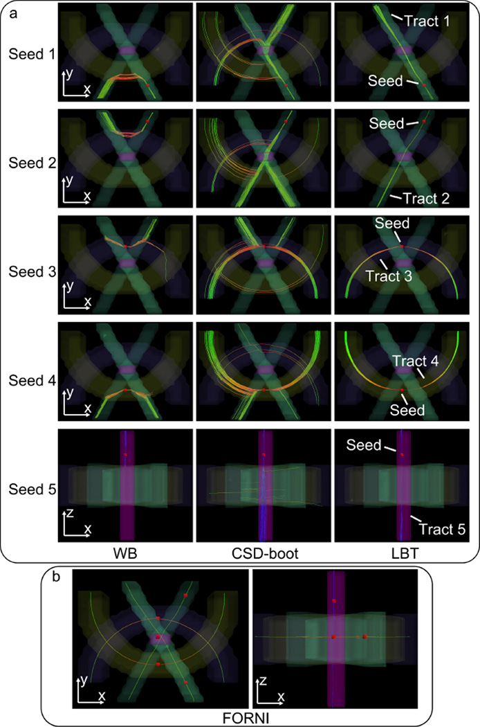
We applied LBT on a 3D digital crossing phantom (see the 3D rendering in Figure 1), where 60 gradient directions with b = 1000 s/mm2 were used to simulate the dMRI acquisition. The phantom consists of five tracts, including four tracts (two straight and two curved ones) in the x-y plane and one tract in the z-direction. In the crossing region with two/three tracts, a two-tensor/three-tensor model was used to simulate the diffusion signals. A Rician noise model was used to create the final simulated diffusion weighted images (DWIs). The signal-to-noise ratio (SNR) on the b0 image (the image without diffusion weighting) is 20, which is a moderate level for simulation (Daducci et al., 2014a) and is close to the SNR in real brain dMRI data. LBT was compared with wild bootstrap (WB) based on the DTI model (Whitcher et al., 2008; Jones, 2008) and the residual bootstrap combined with constrained spherical deconvolution (CSD-boot) (Jeurissen et al., 2011). These two methods were selected for comparison because they are both probabilistic tractography methods based on bootstrap where residuals are resampled, like the proposed method.
Figure 1.
3D renderings of the phantom and probabilistic tractography results. The seed is indicated by the red box. The visualization was created in TrackVis (Wang et al., 2007). (a) Probabilistic tracking results of WB, CSD-boot, and LBT. (b) Deterministic tracking results using FORNI FOs as a tract shape reference.
We first qualitatively evaluated the LBT method and compared it with WB and CSD-boot. For each tract, a seed was placed in a noncrossing region (see Figure 1). One hundred bootstrap FO images were generated for each method, and thus 100 streamlines were generated for each seed in each method. The fiber tracking results are overlaid on the 3D rendering of the tracts in Figure 1. Deterministic fiber tracking results using FOs estimated by FORNI are also shown for a reference of tract shapes. Each segment of each streamline is color-coded with the standard DTI color scheme—red: left–right (x-axis); green: front–back (y-axis); and blue: up–down (z-axis) (Pajevic and Pierpaoli, 1999). It can be seen that WB cannot propagate streamlines through the crossing region; this is because it is based on the DTI model, which is unable to handle crossing FOs. Both CSD-boot and LBT are able to track the crossing fibers; however, CSD-boot has also generated many streamlines that go into undesired pathways. The streamlines produced by LBT are consistent with the FORNI deterministic tracking, and LBT provides a visualization of tracking uncertainty. Note that LBT tracks streamlines through the regions with three crossing tracts, indicating its ability to resolve crossing with more than two fibers.
To quantitatively compare CSD-boot and LBT (WB is not included for comparison because its model cannot handle crossing fibers), we use the error measure proposed in Ye et al. (2016). The means and standard deviations of the average FO error in each bootstrap FO image are 5.56° ± 0.05° and 4.42° ± 0.01° for CSD-boot and LBT, respectively, and LBT produces more accurate FOs. These average FO errors were compared using a Student’s t-test, where the errors of LBT are highly significantly smaller than those of CSD-boot (p < 0.001).
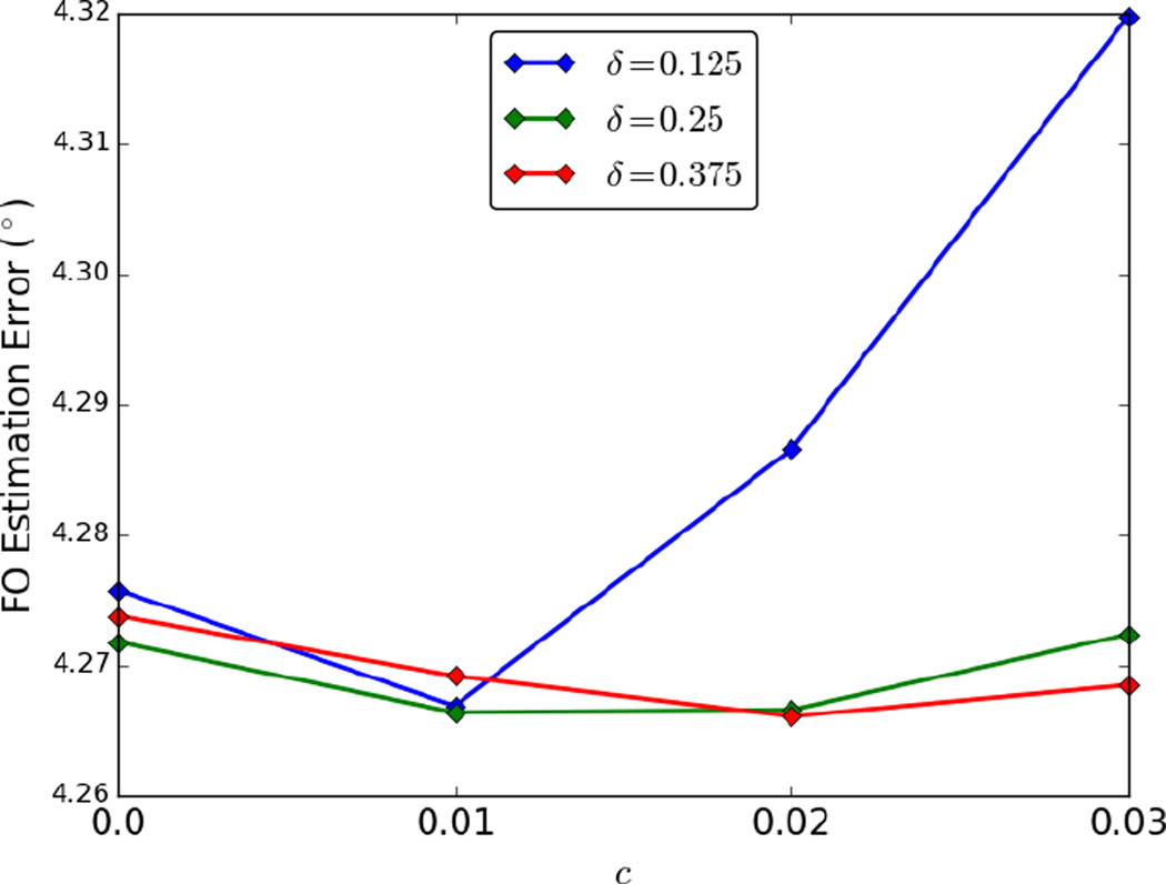
Next, we studied the effect of parameters c and δ used in the bootstrap procedure. Because δ is also related to the number of gradient directions, we added two cases of simulation where 1) 90 gradient directions with b = 1000 s/mm2 (K = 90) and 2) 90 gradient directions each with b = 1000, 2000, 3000 s/mm2 (K = 270) were used. For each parameter combination of c ∈ {0, 0.01, 0.02, 0.03} and δ ∈ {0.125, 0.25, 0.375}, 100 bootstrap FO images were generated for each simulated phantom, resulting in 300 FO images. The average FO errors over these 300 FO images are plotted in Figure 2. Note that c = 0 corresponds to the standard Lasso bootstrap procedure (Knight and Fu, 2000). Overall, the FO errors are robust to the choice of parameters, and we can see that our choice of parameters (c = 0.02 and δ = 0.25) is among the top three in accuracy.
Figure 2.
LBT FO errors with different parameter settings of c and δ.
3.2. In vivo brain dMRI dataset one
Next, LBT was applied to the dMRI data of a human subject. The DWIs were acquired on a 3T MR scanner (Magnetom Trio, Siemens, Erlangen, Germany). The DWIs have 30 gradient directions with b = 1000 s/mm2, and 48 axial slices were acquired for each DWI. The resolution of the DWIs is 2.7 mm isotropic and the matrix size is 84 × 84.
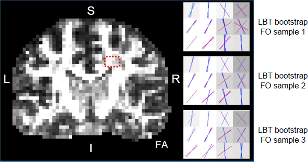
We first demonstrate the samples of FOs generated from LBT in a region that contains the crossing of the corpus callosum (CC) and the corticospinal tract (CST) (see the highlighted region on the FA map in Figure 3). The FOs in the crossing area from three randomly selected bootstrap FO images computed by LBT are shown in Figure 3, and they are color-coded with the standard DTI colormap (red: left–right; green: front–back; and blue: up–down) (Pajevic and Pierpaoli, 1999). In all three FO images, the crossing of the CC and CST is reconstructed; we can also observe that at each voxel the FOs from different bootstrap FO images indicate consistent yet slightly different directions, which characterizes the uncertainty of FO estimation.
Figure 3.
Bootstrap FOs computed by LBT in the crossing region of the CC and CST, which is highlighted by the red dashes on the FA map.
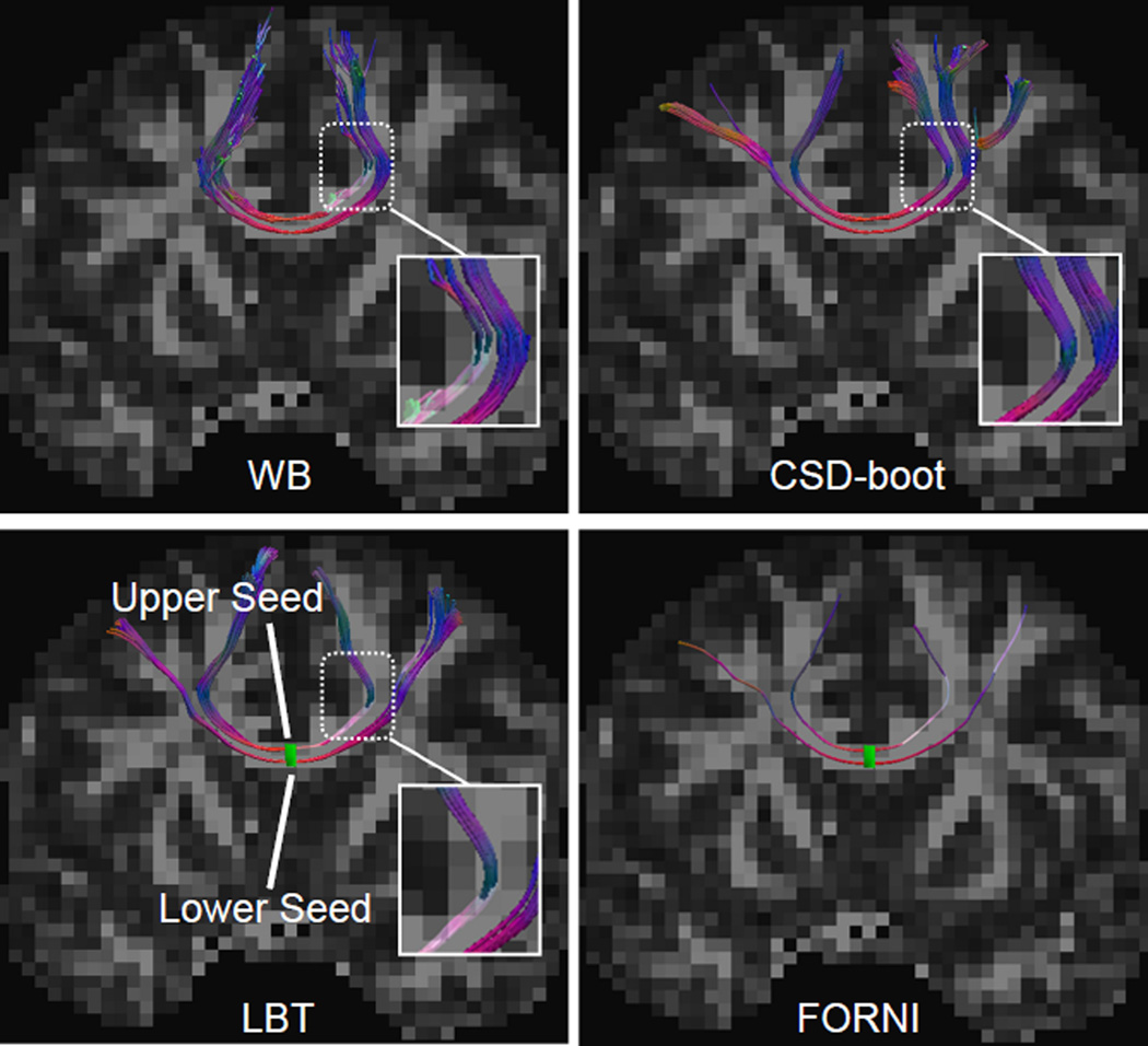
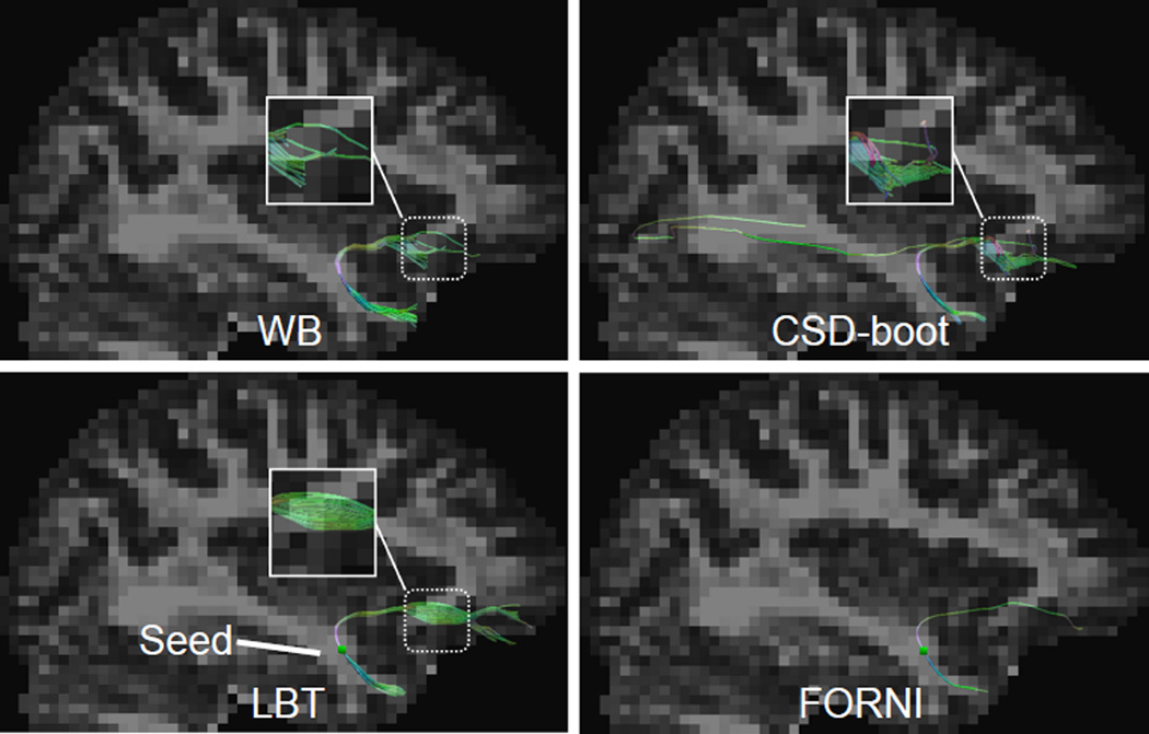
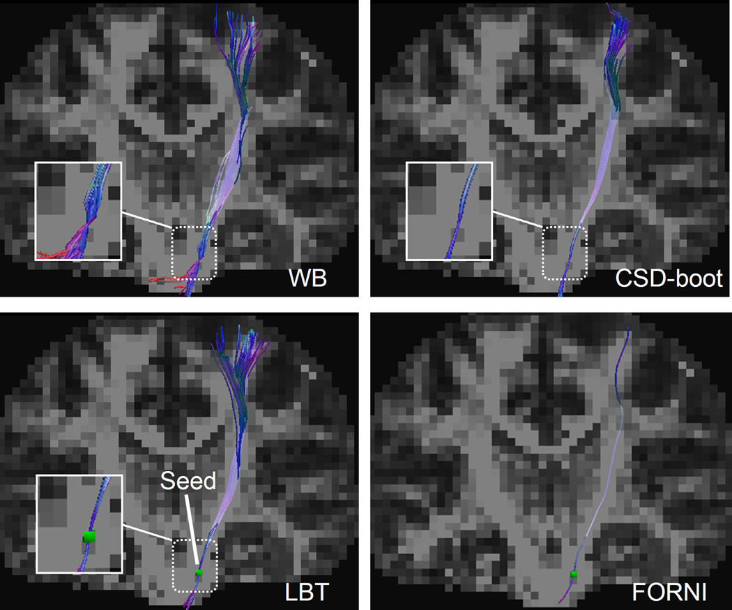
We then demonstrate our results by placing seeds in three characteristic white matter tracts: the CC, the CST, and the uncinate fasciculus (UNC). Seeds were placed in two voxels in the CC and one voxel each in the CST and UNC. For each seed, 100 streamlines were generated by each of the WB, CSD-boot, and LBT methods. The results of LBT are shown and compared with WB and CSD-boot in Figures 4–6 (the visualization was created in TrackVis (Wang et al., 2007)). The streamlines are overlaid on the FA map. Deterministic tracking results using FORNI FOs are also shown for a reference of tract shapes.
Figure 4.
Tractography results seeded in the CC in the coronal view. A deterministic fiber tracking result using FORNI FOs is also shown for a tract shape reference. The upper and lower seeding voxels are represented together by the green rectangle within the LBT and FORNI results in the second row. Note the highlighted zoomed region for comparison.
Figure 6.
Tractography results seeded in the UNC in the sagittal view. A deterministic fiber tracking result using FORNI FOs is also shown for a tract shape reference. The seeding voxel is represented by the green square within the LBT and FORNI results in the second row. Note the highlighted zoomed region for comparison.
In Figure 4, the CC streamlines are shown in the coronal view. The upper and lower seeds correspond to the superior and lateral CC, respectively. WB fails to track the lateral CC because of its DTI model, which cannot propagate streamlines through the crossing of the CC and CST. In the CSD-boot result, part of the lateral CC streamlines are diverted into the pathway of the superior CC. In the LBT result, the superior CC is tracked with the upper seed and the lateral CC is tracked with the lower seed, as it should be.
In Figure 5, the CST streamlines are shown in the coronal view. In the WB result, some streamlines are diverted into the pathway of the middle cerebellar peduncles (the red streamlines). In both CSD-boot and LBT, the CST streamlines are propagated correctly to the cortical area.
Figure 5.
Tractography results seeded in the CST in the coronal view. A deterministic fiber tracking result using FORNI FOs is also shown for a tract shape reference. The seeding voxel is represented by the green square within the LBT and FORNI results in the second row. Note the highlighted zoomed region for comparison.
In Figure 6, the UNC streamlines are shown in the sagittal view. Compared with the WB and CSD-boot results, LBT generates longer UNC streamlines that reach more anterior regions. In addition, in the CSD-boot result, we can see false streamlines reaching the posterior part of the brain.
In Figures 4–6, the LBT results are consistent with the deterministic FORNI results, and LBT provides a probabilistic representation of the tracked streamlines.
3.3. In vivo brain dMRI dataset two: A reproducibility study
We randomly selected five subjects from the Kirby21 data set (Landman et al., 2011) (https://www.nitrc.org/projects/multimodal/) to evaluate the scan-rescan reproducibility of the proposed method. Specifically, two dMRI scans with the same protocol were acquired for each subject on a 3T MR scanner (Achieva, Philips Healthcare, Best, Netherlands). Each dMRI scan contains one b0 image and 32 gradient directions (b = 700 s/mm2), and has 65 axial slices. The data matrix size is 96 × 96 and was reconstructed to 256 × 256 by the scanner, resulting in an in-plane digital resolution of 0.828 mm × 0.828 mm. The slice thickness is 2.2 mm. Detailed description of the dMRI protocol can be found in Landman et al. (2011). We resampled the DWIs so that the resolution is 2.2 mm isotropic. For each subject the second scan was aligned with the first scan by rigidly registering the b0 image, and the gradient table of the second scan was rotated accordingly.
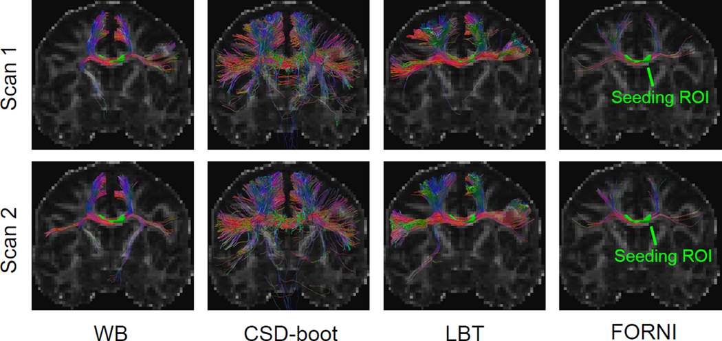
LBT was performed on each dMRI scan. We first qualitatively evaluated the results by focusing on the CC. On each dMRI scan of the first subject, the results of which are representative, we placed a seeding ROI in the CC (see Figure 7) and compared LBT with WB and CSD-boot in Figure 7, where the deterministic fiber tracking results using FOs reconstructed by FORNI are also shown as references. For each seed voxel, 100 streamlines were generated for each probabilistic fiber tracking method. LBT produced both superior and lateral CC, and the shapes of the tracts from the two scans resemble each other. The CC produced by LBT is also consistent with the deterministic tracking results using FOs estimated by FORNI. WB does not always track the lateral CC because its inability to model the crossing CC and CST fibers. Compared with CSD-boot, LBT produces fewer false streamlines that propagate downward; the lateral CC streamlines of LBT are also denser than those of CSD-boot.
Figure 7.
Fiber tracking results computed from the two scans of Subject 1 overlaid on the FA map. Deterministic tracking results using FORNI are also shown for tract shape references.
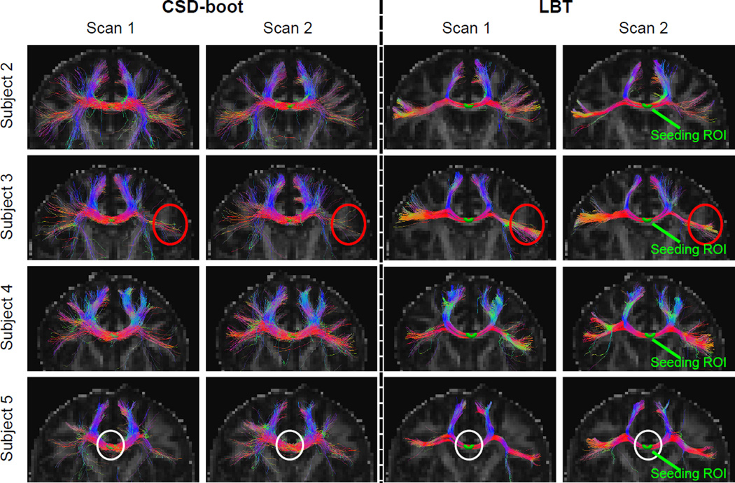
On the remaining four subjects, the qualitative comparison is focused between CSD-boot and LBT, because WB cannot handle crossing fibers. A seeding ROI was placed in the CC on each dMRI scan (see Figure 8), where 100 streamlines were generated for each seeding voxel for each method. For each subject, the CC streamlines produced by LBT are consistent between the two scans, and the superior and lateral CC are properly tracked. Compare with CSD-boot, LBT better tracks the lateral CC (for example, see the region highlighted by the red circle on Subject 3 in Figure 8). We also observe that the uncertainty of the streamlines tracked by LBT is smaller compared with CSD-boot, which is characterized by the thinner yet dense fiber bundles (for example, see the region highlighted by the white circle on Subject 5 in Figure 8).
Figure 8.
CSD-boot and LBT fiber tracking results on Subjects 2–5 (eight scans).
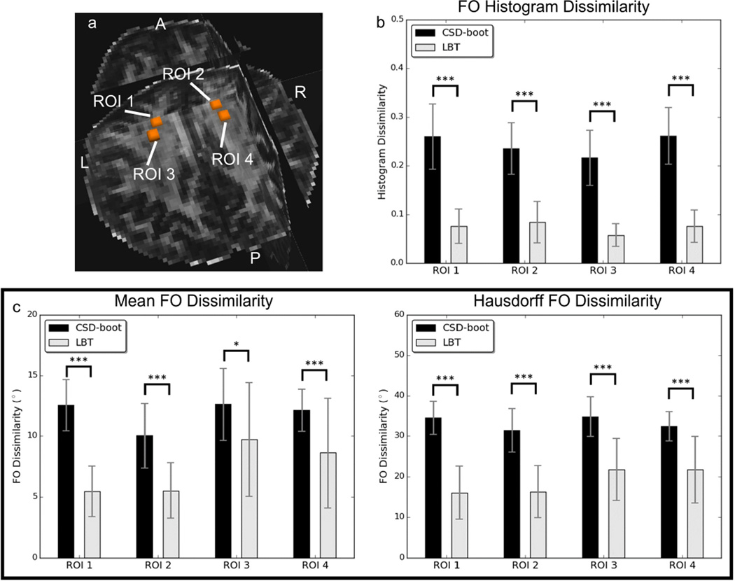
To quantitatively evaluate the reproducibility, for each subject we investigated the dissimilarity between the bootstrap FOs generated from the two scans in ROIs containing the crossing of the CC and CST (see Figure 9(a) for example). Because WB cannot resolve crossing fibers, we focus on the comparison between LBT and CSD-boot.
Figure 9.
FO reproducibility for Subject 1: (a) ROIs replaced in the crossing regions of the CC and CST for FO dissimilarity evaluation, (b) means and standard deviations of the histogram dissimilarity of FOs in each ROI, and (c) means and standard deviations of the FO dissimilarity in each ROI. Asterisks indicate that the difference between the CSD-boot and LBT results is significant using a paired Student’s t-test (*p < 0.05, ***p < 0.001).
First, for each voxel in the selected ROIs, we compute the difference of the histograms of the FOs computed from the two scans. For each FO represented by (ωx, ωy, ωz), it is converted to the spherical coordinate (r, θ, ϕ). Since (ωx, ωy, ωz) is a unit vector, r = 1; we also have 0 ≤ θ ≤ π and 0 ≤ ϕ < 2π. We can compute the 2D histograms of FOs by partitioning θ and ϕ into n and 2n bins, respectively (here we choose n = 10). We denote the histogram by ℋ1 and ℋ2 for the first and second scan, respectively. Note that because of the bi-directionality of the FOs ((ωx, ωy, ωz) and (−ωx, −ωy, −ωz) represent the same FO), for each (ωx, ωy, ωz), (−ωx, −ωy, −ωz) is also used for computing the FO histogram. Suppose the count of bin i is hi,1 and hi,2 for the first and second scan, respectively. We can compute their relative difference dH(hi,1, hi,2) by
| (18) |
(Then, the histogram dissimilarity DH(ℋ1, ℋ2) is measured by the mean of the relative difference of each bin
| (19) |
where B is the number of bootstrap iterations and I is the total number of bins. Smaller DH(ℋ1, ℋ2) indicates more reproducible FO histograms.
Second, at each voxel we compute the differences of the sets of all bootstrap FO configurations computed from the two scans. Suppose the sets of FO configurations for the two scans are ℱ1 and ℱ2, respectively. For each bootstrap FO configuration Ω1 ∈ ℱ1 in the first scan and Ω2 ∈ ℱ2 in the second scan, we can compute their dissimilarity dFO(Ω1, Ω2). Note that each FO configuration can include multiple FOs when fibers cross. Because the FO error computation in Section 3.1 actually measures the difference between estimated and ground truth FOs, we can use the same computation to measure dFO(Ω1, Ω2) by replacing the estimated and ground truth FOs with Ω1 and Ω2. Then, to compute the dissimilarity between the two sets ℱ1 and ℱ2 of FO configurations, we use a mean FO dissimilarity DFOM(ℱ1, ℱ2) and a Hausdorff FO dissimilarity DFOH(ℱ1, ℱ2) defined as
| (20) |
| (21) |
where |ℱ1| and |ℱ2| are the cardinality of ℱ1 and ℱ2, respectively. If ℱ1 and ℱ2 are similar, their dissimilarity dFOM(ℱ1, ℱ2) and dFOH(ℱ1, ℱ2) should be small.
For each dMRI scan, 100 bootstrap FO images were generated using CSD-boot and LBT. On the first representative subject, we placed four ROIs (see Figure 9(a) in regions where the CC and CST cross. The means and standard deviations of the dissimilarity between the bootstrap FOs of the two scans in each ROI are shown in Figure 9(b) and 9(c). For each ROI, the CSD-boot and LBT results were also compared using a paired Student’s t-test. We can see that the dissimilarity between the FOs produced by LBT is significantly smaller than that produced by CSD-boot in all four ROIs, which indicates that LBT produces more reproducible results.
Similar ROIs were also placed on the remaining four subjects. For each subject the reproducibility results using all selected voxels are shown in Figure 10, where CSD-boot and LBT were compared using a paired Student’s t-test. We can see that LBT produces more reproducible FOs with statistical significance.
Figure 10.
Means and standard deviations of FO dissimilarity in regions containing the crossing of the CC and CST for Subjects 2–5: (a) histogram dissimilarity, (b) mean FO dissimilarity, and (c) Hausdorff FO dissimilarity. Asterisks indicate that the difference between the CSD-boot and LBT results is significant using a paired Student’s t-test (***p < 0.001).
4. Discussion
In this work, we use a multi-tensor model with a fixed tensor basis and a sparsity assumption to represent the diffusion signals. In addition to reducing the required gradient directions by using sparsity regularization, this signal model permits the incorporation of FO spatial smoothness for improved FO estimation. Such smoothness is made possible by the explicit relationship between the basis tensors and the FOs, where each PEV of the tensor represents an FO (Ye et al., 2015b, 2016). An important issue in the model is to achieve reasonable estimates of eigenvalues of the basis tensors. Here we have followed the commonly used principles of examining the tensors in regions with high FA (Landman et al., 2012; Tournier et al., 2004), and the procedure can be implemented using publicly available toolboxes, such as Dipy (Garyfallidis et al., 2014).
The Lasso bootstrap provides an approach to estimating the distribution of the diffusion weighted signals. Then, from these synthesized diffusion signals, we use the FORNI algorithm (Ye et al., 2016) to estimate FOs and obtain their distribution, which are then used for fiber tracking. Thus, it is reasonable to consider LBT to be a probabilistic version of FORNI, where uncertainty in fiber tracking is quantified. In the fiber tracking results, we have observed the consistency between the probabilistic LBT and deterministic FORNI results. Furthermore, LBT provides additional information about the uncertainty of the tracked streamlines.
The major difference between the conventional residual bootstrap, such as the one used in Jeurissen et al. (2011), and the Lasso bootstrap is the centering of residuals. As discussed in Chatterjee and Lahiri (2011), the residuals must be centered for the validity of the residual bootstrap. In the conventional bootstrap settings, the condition automatically holds; however, due to the incorporation of an ℓ1-norm penalty, the residuals are not centered in the Lasso model. Thus, the conventional residual bootstrap without centering the residuals is inappropriate and a Lasso bootstrap strategy that centers the residuals is needed.
As discussed in Chatterjee and Lahiri (2011), the residual bootstrap is consistent for the Lasso model without scaling, and the rescaling effect is asymptotically negligible. Therefore, in this work the residuals are not corrected for leverage, and we believe the correction would produce similar results.
We assume that the noise in each gradient direction is independent and identically distributed, which is a common and sensible assumption (Jian and Vemuri, 2007). Thus, we only deal with homoscedastic noise, as does the modified Lasso bootstrap in Chatterjee and Lahiri (2011). For Lasso models with heteroscedastic noise, it is possible to use other bootstrap strategies such as Camponovo (2015) and Wagener and Dette (2012).
Most of the parameters in this work are determined using the default parameters of existing algorithms (e.g., the parameters in FO estimation) or commonly used values (e.g., fiber tracking parameters). In particular, α and β in the FO estimation step control the spatial consistency and sparsity of FOs, respectively. Increasing α leads to better spatial consistency of FOs. Larger β encourages a smaller number of FOs, and smaller β may prefer crossing FOs to a single FO. In the bootstrap procedure, we have shown in the phantom experiments that the results are robust to the selection of parameters c and δ and our choice achieves good accuracy. A larger number of bootstrap samples could provide a more accurate estimation of the uncertainty but increases the computational burden. Here we followed Yap et al. (2014) to use 100 bootstrap samples for each seed to demonstrate the results. It may be fruitful to explore the optimal number of bootstrap samples in a data-driven way that reaches a balance between speed and accuracy.
The experiments were performed using a 16-core Linux machine. For the brain dMRI datasets in Sections 3.2 and 3.3, where the resolution is between 2 mm and 3 mm, 100 bootstrap iterations took around 40 hours. Note that the process of generating each bootstrap FO image is parallelizable, and it is possible to explore the use of distributed computing, such as computer clusters, for acceleration.
5. Summary and Conclusion
In this work, we have presented a probabilistic tractography method LBT based on a Lasso bootstrap scheme. A fixed tensor basis is used to model the diffusion signals in a Lasso formulation. The modified Lasso bootstrap (Chatterjee and Lahiri, 2011) is then used to synthesize diffusion signals, from which the FOs can be estimated using an improved estimation algorithm (Ye et al., 2015b, 2016) that incorporates spatial consistency of FOs. Probabilistic streamlining fiber tracking is performed with these FOs. The LBT algorithm was evaluated on simulated and real dMRI data, where it outperforms other state-of-the-art methods.
Highlights.
We propose a probabilistic tractography method named Lasso bootstrap tractography.
The distribution of diffusion signals is estimated using modified Lasso bootstrap.
We compute fiber orientations (FOs) using an algorithm incorporating FO smoothness.
Qualitative and quantitative evaluation was performed on simulated and real data.
Acknowledgments
This work is supported in part by NIH/NINDS 5R01NS056307, NSFC 61601461, and the “100 Talents Program” of the Chinese Academy of Sciences.
Footnotes
Publisher's Disclaimer: This is a PDF file of an unedited manuscript that has been accepted for publication. As a service to our customers we are providing this early version of the manuscript. The manuscript will undergo copyediting, typesetting, and review of the resulting proof before it is published in its final citable form. Please note that during the production process errors may be discovered which could affect the content, and all legal disclaimers that apply to the journal pertain.
References
- Aranda R, Rivera M, Ramirez-Manzanares A. A flocking based method for brain tractography. Medical Image Analysis. 2014;18:515–530. doi: 10.1016/j.media.2014.01.009. [DOI] [PubMed] [Google Scholar]
- Basser P, Mattiello J, LeBihan D. MR diffusion tensor spectroscopy and imaging. Biophysical Journal. 1994;66:259–267. doi: 10.1016/S0006-3495(94)80775-1. [DOI] [PMC free article] [PubMed] [Google Scholar]
- Basser P, Pajevic S, Pierpaoli C, Duda J, Aldroubi A. In vivo fiber tractography using DT-MRI data. Magnetic Resonance in Medicine. 2000;44:625–632. doi: 10.1002/1522-2594(200010)44:4<625::aid-mrm17>3.0.co;2-o. [DOI] [PubMed] [Google Scholar]
- Behrens T, Berg H, Jbabdi S, Rushworth M, Woolrich M. Probabilistic diffusion tractography with multiple fibre orientations: What can we gain? NeuroImage. 2007;34:144–155. doi: 10.1016/j.neuroimage.2006.09.018. [DOI] [PMC free article] [PubMed] [Google Scholar]
- Berman J, Chung S, Mukherjee P, Hess C, Han E, Henry R. Probabilistic streamline q-ball tractography using the residual bootstrap. NeuroImage. 2008;39:215–222. doi: 10.1016/j.neuroimage.2007.08.021. [DOI] [PubMed] [Google Scholar]
- Bilgic B, Setsompop K, Cohen-Adad J, Yendiki A, Wald LL, Adalsteinsson E. Accelerated diffusion spectrum imaging with compressed sensing using adaptive dictionaries. Magnetic Resonance in Medicine. 2012;68:1747–1754. doi: 10.1002/mrm.24505. [DOI] [PMC free article] [PubMed] [Google Scholar]
- Camponovo L. On the validity of the pairs bootstrap for lasso estimators. Biometrika. 2015;102:981–987. [Google Scholar]
- Catheline G, Periot O, Amirault M, Braun M, Dartigues JF, Auriacombe S, Allard M. Distinctive alterations of the cingulum bundle during aging and alzheimers disease. Neurobiology of Aging. 2010;31:1582–1592. doi: 10.1016/j.neurobiolaging.2008.08.012. [DOI] [PubMed] [Google Scholar]
- Chatterjee A, Lahiri S. Asymptotic properties of the residual bootstrap for Lasso estimators. Proceedings of the American Mathematical Society. 2010;138:4497–4509. [Google Scholar]
- Chatterjee A, Lahiri S. Bootstrapping Lasso estimators. Journal of the American Statistical Association. 2011;106:608–625. [Google Scholar]
- Chung S, Lu Y, Henry R. Comparison of bootstrap approaches for estimation of uncertainties of DTI parameters. NeuroImage. 2006;33:531–541. doi: 10.1016/j.neuroimage.2006.07.001. [DOI] [PubMed] [Google Scholar]
- Daducci A, Canales-Rodriguez EJ, Descoteaux M, Garyfallidis E, Gur Y, Lin YC, Mani M, Merlet S, Paquette M, Ramirez-Manzanares A, Reisert M, Reis Rodrigues P, Sepehrband F, Caruyer E, Choupan J, Deriche R, Jacob M, Menegaz G, Prckovska V, Rivera M, Wiaux Y, Thiran JP. Quantitative comparison of reconstruction methods for intra-voxel fiber recovery from diffusion MRI. IEEE Transactions on Medical Imaging. 2014a;33:384–399. doi: 10.1109/TMI.2013.2285500. [DOI] [PubMed] [Google Scholar]
- Daducci A, Van De Ville D, Thiran JP, Wiaux Y. Sparse regularization for fiber ODF reconstruction: From the suboptimality of ℓ2 and ℓ1 priors to ℓ0. Medical Image Analysis. 2014b;18:820–833. doi: 10.1016/j.media.2014.01.011. [DOI] [PubMed] [Google Scholar]
- Descoteaux M, Deriche R, Knösche TR, Anwander A. Deterministic and probabilistic tractography based on complex fibre orientation distributions. IEEE Transactions on Medical Imaging. 2009;28:269–286. doi: 10.1109/TMI.2008.2004424. [DOI] [PubMed] [Google Scholar]
- Efron B. Bootstrap methods: another look at the jackknife. The Annals of Statistics. 1979;7:1–26. [Google Scholar]
- Garyfallidis E, Brett M, Amirbekian B, Rokem A, Van Der Walt S, Descoteaux M, Nimmo-Smith I, Contributors D. Dipy, a library for the analysis of diffusion MRI data. Frontiers in Neuroinformatics. 2014;8:1–17. [Google Scholar]
- Hess C, Mukherjee P, Han E, Xu D, Vigneron D. Q-ball reconstruction of multimodal fiber orientations using the spherical harmonic basis. Magnetic Resonance in Medicine. 2006;56:104–117. doi: 10.1002/mrm.20931. [DOI] [PubMed] [Google Scholar]
- Horn A, Ostwald D, Reisert M, Blankenburg F. The structural–functional connectome and the default mode network of the human brain. NeuroImage. 2014;102:142–151. doi: 10.1016/j.neuroimage.2013.09.069. [DOI] [PubMed] [Google Scholar]
- Jeurissen B, Leemans A, Jones D, Tournier JD, Sijbers J. Probabilistic fiber tracking using the residual bootstrap with constrained spherical deconvolution. Human Brain Mapping. 2011;32:461–479. doi: 10.1002/hbm.21032. [DOI] [PMC free article] [PubMed] [Google Scholar]
- Jian B, Vemuri BC. A unified computational framework for deconvolution to reconstruct multiple fibers from diffusion weighted MRI. IEEE Transactions on Medical Imaging. 2007;26:1464–1471. doi: 10.1109/TMI.2007.907552. [DOI] [PMC free article] [PubMed] [Google Scholar]
- Johansen-Berg H, Behrens TEJ. Diffusion MRI: from quantitative measurement to in vivo neuroanatomy. Waltham: Academic Press; 2013. [Google Scholar]
- Jones D. Tractography gone wild: probabilistic fibre tracking using the wild bootstrap with diffusion tensor MRI. IEEE Transactions on Medical Imaging. 2008;27:1268–1274. doi: 10.1109/TMI.2008.922191. [DOI] [PubMed] [Google Scholar]
- Jones DK. Determining and visualizing uncertainty in estimates of fiber orientation from diffusion tensor MRI. Magnetic Resonance in Medicine. 2003;49:7–12. doi: 10.1002/mrm.10331. [DOI] [PubMed] [Google Scholar]
- Knight K, Fu W. Asymptotics for lasso-type estimators. The Annals of Statistics. 2000;28:1356–1378. [Google Scholar]
- Landman BA, Bogovic JA, Wan H, ElShahaby FEZ, Bazin PL, Prince JL. Resolution of crossing fibers with constrained compressed sensing using diffusion tensor MRI. NeuroImage. 2012;59:2175–2186. doi: 10.1016/j.neuroimage.2011.10.011. [DOI] [PMC free article] [PubMed] [Google Scholar]
- Landman BA, Huang AJ, Gifford A, Vikram DS, Lim IAL, Farrell JA, Bogovic JA, Hua J, Chen M, Jarso S, Smith SA, Joel S, Mori S, Pekar JJ, Barker PB, Prince JL, van Zijl PC. Multi-parametric neuroimaging reproducibility: A 3-T resource study. NeuroImage. 2011;54:2854–2866. doi: 10.1016/j.neuroimage.2010.11.047. doi: http://dx.doi.org/10.1016/j.neuroimage.2010.11.047. [DOI] [PMC free article] [PubMed] [Google Scholar]
- Lazar M, Alexander AL. Bootstrap white matter tractography (BOOT-TRAC) NeuroImage. 2005;24:524–532. doi: 10.1016/j.neuroimage.2004.08.050. [DOI] [PubMed] [Google Scholar]
- Malcolm JG, Shenton ME, Rathi Y. Filtered multitensor tractography. IEEE Transactions on Medical Imaging. 2010;29:1664–1675. doi: 10.1109/TMI.2010.2048121. [DOI] [PMC free article] [PubMed] [Google Scholar]
- Michailovich O, Rathi Y, Dolui S. Spatially regularized compressed sensing for high angular resolution diffusion imaging. IEEE Transactions on Medical Imaging. 2011;30:1100–1115. doi: 10.1109/TMI.2011.2142189. [DOI] [PMC free article] [PubMed] [Google Scholar]
- Mori S, Crain B, Chacko V, Van Zijl P. Three-dimensional tracking of axonal projections in the brain by magnetic resonance imaging. Annals of Neurology. 1999;45:265–269. doi: 10.1002/1531-8249(199902)45:2<265::aid-ana21>3.0.co;2-3. [DOI] [PubMed] [Google Scholar]
- Mori S, Wakana S, van Zijl PCM, Nagae-Poetscher LM. MRI Atlas of Human White Matter. Amsterdam: Elsevier Science; 2005. [Google Scholar]
- Pajevic S, Pierpaoli C. Color schemes to represent the orientation of anisotropic tissues from diffusion tensor data: application to white matter fiber tract mapping in the human brain. Magnetic Resonance in Medicine. 1999;42:526–540. [PubMed] [Google Scholar]
- Parker GJM, Haroon HA, Wheeler-Kingshott CAM. A framework for a streamline-based probabilistic index of connectivity (PICo) using a structural interpretation of MRI diffusion measurements. Journal of Magnetic Resonance Imaging. 2003;18:242–254. doi: 10.1002/jmri.10350. [DOI] [PubMed] [Google Scholar]
- Phillips OR, Nuechterlein KH, Clark KA, Hamilton LS, Asarnow RF, Hageman NS, Toga AW, Narr KL. Fiber tractography reveals disruption of temporal lobe white matter tracts in schizophrenia. Schizophrenia Research. 2009;107:30–38. doi: 10.1016/j.schres.2008.10.019. [DOI] [PMC free article] [PubMed] [Google Scholar]
- Ramirez-Manzanares A, Rivera M, Vemuri BC, Carney P, Mareci T. Diffusion basis functions decomposition for estimating white matter intravoxel fiber geometry. IEEE Transactions on Medical Imaging. 2007;26:1091–1102. doi: 10.1109/TMI.2007.900461. [DOI] [PubMed] [Google Scholar]
- Rathi Y, Michailovich O, Laun F, Setsompop K, Grant PE, Westin CF. Multi-shell diffusion signal recovery from sparse measurements. Medical Image Analysis. 2014;18:1143–1156. doi: 10.1016/j.media.2014.06.003. [DOI] [PMC free article] [PubMed] [Google Scholar]
- Ratnarajah N, Simmons A, Bertoni M, Hojjatoleslami A. Two-tensor model-based bootstrapping on classified tensor morphologies: estimation of uncertainty in fiber orientation and probabilistic tractography. Magnetic Resonance Imaging. 2013;31:296–312. doi: 10.1016/j.mri.2012.07.004. [DOI] [PubMed] [Google Scholar]
- de Schotten MT, Bizzi A, Dell’Acqua F, Allin M, Walshe M, Murray R, Williams SC, Murphy DGM, Catani M. Atlasing location, asymmetry and inter-subject variability of white matter tracts in the human brain with MR diffusion tractography. NeuroImage. 2011;54:49–59. doi: 10.1016/j.neuroimage.2010.07.055. [DOI] [PubMed] [Google Scholar]
- Tibshirani R. Regression shrinkage and selection via the lasso. Journal of the Royal Statistical Society. Series B (Methodological) 1996;58:267–288. [Google Scholar]
- Tournier J, Calamante F, Connelly A. Robust determination of the fibre orientation distribution in diffusion MRI: non-negativity constrained super-resolved spherical deconvolution. NeuroImage. 2007;35:1459–1472. doi: 10.1016/j.neuroimage.2007.02.016. [DOI] [PubMed] [Google Scholar]
- Tournier JD, Calamante F, Gadian DG, Connelly A. Direct estimation of the fiber orientation density function from diffusion-weighted MRI data using spherical deconvolution. NeuroImage. 2004;23:1176–1185. doi: 10.1016/j.neuroimage.2004.07.037. [DOI] [PubMed] [Google Scholar]
- Tuch D, Reese T, Wiegell M, Makris N, Belliveau J, Wedeen V. High angular resolution diffusion imaging reveals intravoxel white matter fiber heterogeneity. Magnetic Resonance in Medicine. 2002;48:577–582. doi: 10.1002/mrm.10268. [DOI] [PubMed] [Google Scholar]
- Vishwas MS, Chitnis T, Pienaar R, Healy BC, Grant PE. Tract-based analysis of callosal, projection, and association pathways in pediatric patients with multiple sclerosis: a preliminary study. American Journal of Neuroradiology. 2010;31:121–128. doi: 10.3174/ajnr.A1776. [DOI] [PMC free article] [PubMed] [Google Scholar]
- Wagener J, Dette H. Bridge estimators and the adaptive lasso under heteroscedasticity. Mathematical Methods of Statistics. 2012;21:109–126. [Google Scholar]
- Wang B, Fan Y, Lu M, Li S, Song Z, Peng X, Zhang R, Lin Q, He Y, Wang J, Huang R. Brain anatomical networks in world class gymnasts: A DTI tractography study. NeuroImage. 2013;65:476–487. doi: 10.1016/j.neuroimage.2012.10.007. [DOI] [PubMed] [Google Scholar]
- Wang R, Benner T, Sorensen AG, Wedeen VJ. Diffusion toolkit: a software package for diffusion imaging data processing and tractography. Proc Intl Soc Mag Reson Med. 2007;15:3720. [Google Scholar]
- Wedeen VJ, Hagmann P, Tseng WYI, Reese TG, Weisskoff RM. Mapping complex tissue architecture with diffusion spectrum magnetic resonance imaging. Magnetic Resonance in Medicine. 2005;54:1377–1386. doi: 10.1002/mrm.20642. [DOI] [PubMed] [Google Scholar]
- Whitcher B, Tuch D, Wisco J, Sorensen A, Wang L. Using the wild bootstrap to quantify uncertainty in diffusion tensor imaging. Human Brain Mapping. 2008;29:346–362. doi: 10.1002/hbm.20395. [DOI] [PMC free article] [PubMed] [Google Scholar]
- Yap PT, An H, Chen Y, Shen D. Uncertainty estimation in diffusion MRI using the nonlocal bootstrap. IEEE Transactions on Medical Imaging. 2014;33:1627–1640. doi: 10.1109/TMI.2014.2320947. [DOI] [PMC free article] [PubMed] [Google Scholar]
- Ye C, Carass A, Murano E, Stone M, Prince JL. Bayesian and grAphical Models for Biomedical Imaging. Springer; 2014. A Bayesian approach to distinguishing interdigitated muscles in the tongue from limited diffusion weighted imaging; pp. 13–24. volume 8677 of Lecture Notes in Computer Science. [DOI] [PMC free article] [PubMed] [Google Scholar]
- Ye C, Glaister J, Prince JL. Probabilistic fiber tracking using a modified Lasso bootstrap method; 2015 IEEE 12th International Symposium on Biomedical Imaging (ISBI); 2015a. pp. 943–946. [DOI] [PMC free article] [PubMed] [Google Scholar]
- Ye C, Zhuo J, Gullapalli RP, Prince JL. Estimation of fiber orientations using neighborhood information; MICCAI Workshop on Computational Diffusion MRI; 2015b. [DOI] [PMC free article] [PubMed] [Google Scholar]
- Ye C, Zhuo J, Gullapalli RP, Prince JL. Estimation of fiber orientations using neighborhood information. Medical Image Analysis. 2016;32:243–256. doi: 10.1016/j.media.2016.05.008. doi: http://dx.doi.org/10.1016/j.media.2016.05.008. [DOI] [PMC free article] [PubMed] [Google Scholar]
- Yeh FC, Wedeen VJ, Tseng WYI. Generalized q-sampling imaging. IEEE Transactions on Medical Imaging. 2010;29:1626–1635. doi: 10.1109/TMI.2010.2045126. [DOI] [PubMed] [Google Scholar]


