Random Forest Regression for Magnetic Resonance Image Synthesis

Abstract

By choosing different pulse sequences and their parameters, magnetic resonance imaging (MRI) can generate a large variety of tissue contrasts. This very flexibility, however, can yield inconsistencies with MRI acquisitions across datasets or scanning sessions that can in turn cause inconsistent automated image analysis. Although image synthesis of MR images has been shown to be helpful in addressing this problem, an inability to synthesize both T₂-weighted brain images that include the skull and FLuid Attenuated Inversion Recovery (FLAIR) images has been reported. The method described herein, called REPLICA, addresses these limitations. REPLICA is a supervised random forest image synthesis approach that learns a nonlinear regression to predict intensities of alternate tissue contrasts given specific input tissue contrasts. Experimental results include direct image comparisons between synthetic and real images, results from image analysis tasks on both synthetic and real images, and comparison against other state-of-the-art image synthesis methods. REPLICA is computationally fast, and is shown to be comparable to other methods on tasks they are able to perform. Additionally REPLICA has the capability to synthesize both T₂-weighted images of the full head and FLAIR images, and perform intensity standardization between different imaging datasets.

Graphical abstract

1. Introduction

Magnetic resonance imaging (MRI) is the dominant imaging modality for studying neuroanatomy. In MRI, the soft tissues in the brain can be imaged with different tissue contrasts by using different pulse sequences. Pulse sequences like magnetization-prepared gradient echo (MPRAGE) and spoiled gradient recalled (SPGR) produce a T₁-weighted (T₁w) tissue contrast which has good image contrast between gray matter (GM) and white matter (WM) tissues. T₁w pulse sequences are used extensively as inputs for automated segmentation (Prastawa et al., 2004; Roy et al., 2012) and cortical reconstruction algorithms (Dale and Fischl, 1999; Han et al., 2004; Shiee et al., 2014). Pulse sequences like dual spin echo (DSE) are used to produce P_D-weighted (P_Dw) and T₂-weighted (T₂w) tissue contrasts, which are useful for visualizing tissue abnormalities like lesions. Fluid attenuated inversion recovery (FLAIR) is a T₂w pulse sequence that uses inversion recovery as a mechanism to enhance the image contrast of white matter lesions (WMLs). Multiple sclerosis is an example of a disease whose study benefits from the use of FLAIR imaging to detect and quantify WMLs (Llado et al., 2012).

MRI thus provides us with a panoply of neuroimaging options via pulse sequences, each of which provides a unique view of the intrinsic MR parameters. The inherent diversity of MRI is a boon to diagnosticians but can prove to be a challenge for automated image analysis. In clinical scenarios, where the scanning time for a patient is always limited and generally expensive, the number of tissue contrasts that can be acquired is limited. Certain pulse sequences like MPRAGE and SPGR can be acquired at a high resolution (1 mm³ or smaller voxel size) in a matter of 3–10 minutes. Sequences like DSE and FLAIR, which have long repetition times (TR) or inversion times (TI), are typically acquired at a lower resolution or, worse, not at all. If acquired at a lower resolution, these images are usually upsampled to match the highest resolution of the other modalities while performing multimodal image analysis. This makes it difficult to accurately understand and visualize the underlying neuroanatomy. MRI acquisitions can also be affected by artifacts that render them unusable (Stuckey et al., 2007). Such missing or inconsistent data affects the consistency of image processing applied to the whole dataset. In order to carry out consistent and automated image processing on such datasets, we propose to use image synthesis to generate images that fill the gaps in the data and/or enhance its quality.

We define image synthesis as an intensity transformation applied to a given set of input images to generate a new image with a specific tissue contrast. In general, we use image synthesis as a preprocessing step that takes place before applying more complex image processing algorithms such as segmentation and registration. Synthesis of an MR image that is perfectly identical to its true counterpart is not possible and therefore synthetic images are not intended to be used for diagnostic purposes. Our goal is to generate synthetic images that are close enough approximations to real images so that further automated image processing and analysis steps are either enabled or improved.

The practice of image synthesis has been gaining attention recently (Rousseau, 2008; Roy et al., 2010a,b; Rousseau, 2010; Roy et al., 2011; Roohi et al., 2012; Jog et al., 2013a; Rousseau and Studholme, 2013; Konukoglu et al., 2013; Ye et al., 2013; Iglesias et al., 2013; Roy et al., 2013a,b; Jog et al., 2014a; Roy et al., 2014; Burgos et al., 2014; van Tulder and de Bruijne, 2015; Jog et al., 2015a; Cardoso et al., 2015; Van Nguyen et al., 2015; Bahrami, Khosro and Shi, Feng and Zong, Xiaopeng and Shin, Hae Won and An, Hongyu and Shen, Dinggang, 2015; Zikic et al., 2014) and the number of applications where image synthesis methods are being used is also growing. Synthesis of modalities differs from the data imputation literature (Hor and Moradi, 2015) in that the main goal is synthesis of the missing modality as opposed to classification in the absence of it. Image synthesis methods can be classified into two broad categories: (1) registration-based methods and (2) intensity transformation-based methods. Registration-based synthesis originated in the work of Miller et al. (1993), where image synthesis was achieved by spatially aligning a single subject image and an image within a co-registered collection of images, which we call an atlas. Given a subject image b₁ of modality (or tissue contrast) M₁ and a pair of co-registered atlas images a₁ and a₂ of modalities M₁ and M₂ respectively; a₁ is deformably registered to b₁ and the same transformation is applied to a₂ to generate ${\widehat{b}}_2$ of modality M₂. Burgos et al. (2014) extended this approach by introducing multi-atlas registration and intensity fusion to create the final synthesized image; they applied the method to synthesize computed tomography (CT) images from corresponding MR images. A variant of this approach was recently proposed by Cardoso et al. (2015) where a generative model learned using multiple atlases was used for outlier classification and image synthesis. Using registration for synthesis can lead to significant errors in the finer regions of the brain such as the cerebral cortex, where registration is not always accurate. Registration-based synthesis also fails in the presence of abnormal tissue anatomy since the atlases do not have pathology in the same locations as the subjects.

One of the first approaches using an intensity transformation for synthesis is called image analogies, as described by Hertzmann et al. (2001). In this approach, the atlas images a₁ and a₂ are assumed to be related by an unknown filter h as a₂ = h * a₁. Given a subject image b₁, the goal is to synthesize ${\widehat{b}}_2$, which should ideally be equal to h * b₁. This is achieved by forming ${\widehat{b}}_2$ patch-by-patch. A patch in b₁ is considered for synthesis and its nearest neighbor in the set of patches extracted from a₁ is found. The corresponding a₂ patch is picked and placed to form the patch in ${\widehat{b}}_2$. This synthesis approach is wrapped in a multi-resolution framework, and attempts to mimic the action of the filter h. The image analogies method has been applied in MR synthesis (Iglesias et al., 2013), where synthesis of an alternate tissue contrast was shown to improve registration. Image synthesis has also been framed and solved as a sparse dictionary reconstruction problem called MIMECS (Roy et al., 2011, 2013a). Patches extracted from the atlas image a₁ form a dictionary, which is used to describe the patches in the subject image b₁ as a sparse, linear combination of its atoms. The same corresponding patches from a₂ are combined with the same linear coefficients to synthesize patches in ${\widehat{b}}_2$. The paper by Roy et al. (2013a) demonstrated multiple applications of synthesis including intensity standardization and improved registration. A generative model of synthesis using patches was described by Roy et al. (2014), which was used to synthesize CT images from ultra-short echo time (UTE) MR images.

Intensity transformation approaches such as image analogies and MIMECS have long runtimes. Image analogies must find a nearest neighbor patch for each voxel while using its synthesized neighbor voxel during synthesis, and this process cannot be parallelized. MIMECS must solve a sparse reconstruction problem at each voxel, which can be parallelized but this is a relatively long step, and without this extra programming it is very time consuming. The range of application of these methods is also somewhat limited. For example, MIMECS was shown to be ill-suited for the purpose of synthesizing FLAIR images (Roy et al., 2013a). With better training data we have improved MIMECS FLAIR synthesis but many deficiencies still remain.

In this paper, we describe an intensity transformation-based image synthesis approach that uses a nonlinear regression in feature space to predict the intensity in the target modality (tissue contrast). We use local patches and additional context features within a multi-resolution framework (cf. Hertzmann et al. (2001)) to form our feature space. The nonlinear regression is learned using a regression ensemble based on random forests (Breiman, 1996). We call our approach Regression Ensembles with Patch Learning for Image Contrast Agreement or REPLICA. Our approach is computationally much faster than existing approaches and delivers comparable and sometimes better synthesis results. It can also be used to synthesize FLAIR images, and is able to synthesize T₂w images with skull; capabilities that have not been demonstrated by other intensity transformation synthesis approaches.

Aspects of REPLICA have appeared in previous conference publications (Jog et al., 2013a, 2014b) where we demonstrated its use in example-based super-resolution and intensity standardization scenarios. A previous version of REPLICA was used as part of another image synthesis strategy in Jog et al. (2015b). In this paper, we provide a complete description of REPLICA including its use of a multi-resolution framework and context features. We also include in-depth experiments showcasing the efficacy of synthesis both by direct comparison to real images and by comparison of further processing steps that use synthetic images as opposed to real images.

This paper is organized as follows. We describe the REPLICA method in Section 2. Parameter selection is described in supplementary material provided along with this manuscript. Results are shown in Section 3, where we show synthesis of T₂w and FLAIR images. We also justify our choice of features and the necessity of a multi-resolution framework by demonstrating results for the relatively challenging task of synthesizing a whole head image (i.e. without skullstripping). We demonstrate an intensity standardization application in which we reconcile two different imaging datasets to provide a more consistent segmentation. A brief conclusion including a discussion of future work is provided in Section 4.

2. Method

Let $ℬ=\left\{b_1,b_2,\dots ,b_m\right\}$ be a subject image set, imaged with pulse sequences Φ₁,…, Φ_m. This set contains m images from m different pulse sequences such as MPRAGE, FLAIR, DSE, etc. We sometimes refer to these different pulse sequences as “modalities” since they generate different tissue contrasts with images that often appear very different from one another. Let $\mathcal{A}=\left\{a_1,a_2,\dots ,a_m,a_r\right\}$ be the atlas collection generated by the pulse sequences Φ₁,…, Φ_m (which are the same as those of the subject images) and Φ_r, where Φ_r is the target atlas modality that we want to synthesize from the subject set. The atlas collection can contain imaging data from more than one individual but for simplicity in this description we assume that there is only one individual in the atlas.

Our goal is to synthesize a subject image ${\widehat{b}}_r$ that has the same tissue contrast as the atlas image a_r. We frame this problem as a nonlinear regression where we want to predict the intensities of ${\widehat{b}}_r$, voxel-by-voxel. This nonlinear regression is learned using random forest regression (Breiman, 1996). Training data is generated using the atlas image set by extracting feature vectors f(x) at voxel locations x in the atlas image domain Ω. The random forest is trained so that these features predict the voxel intensity a_r(x) of the atlas target modality. Once trained, these features are extracted from the subject image and the random forest is used to predict ${\widehat{b}}_r$. These steps are described in detail below.

2.1. Features

Generating a synthetic image of modality Φ_r from modalities Φ₁,…, Φ_m involves calculating an intensity transformation that jointly considers features in these modalities to predict the intensities in a_r generated by Φ_r. If we consider an individual voxel intensity as the only feature then in most realistic image synthesis scenarios the intensity transformation is not a one-to-one function between the input and target modality voxel intensities. For example, in T₁w images, the cerebrospinal fluid (CSF) and bone are both imaged as dark regions. However in corresponding T₂w images, the CSF is bright and the bone is dark (due to a very small T₂ and a negligible signal). Thus the same T₁w dark intensities have two very different mappings in the T₂w range. A regression trained on such ambiguous data and applied to unknown, test T₁w intensities is bound to yield substantial errors.

One way to reduce such errors is to add additional features associated with each voxel x ∈ Ω. Previous approaches like image analogies (Hertzmann et al., 2001) and MIMECS (Roy et al., 2013a) used small image patches (usually 3 × 3 × 3 voxels centered on x) as features. Small patches add some spatial context to a single voxel, but they are still often unable to resolve the ambiguity of a one-to-many mapping from feature space to the target modality intensity. Registration-based approaches (Burgos et al., 2014; Cardoso et al., 2015) attempt to solve this issue by carrying over the spatial context from the atlas images to the subject image via registration under the assumption that after registration, the intensity transformation is simple enough to be learned by using small patches. We address this problem in two ways, first by using a multi-resolution framework and second by adding remote features which we call context features, as described next.

2.1.1. Multi-resolution Features

For each image a_i in the atlas set, we construct a Gaussian pyramid (using σ = 1 voxel) on scales s ∈ {1,…, S} (Hertzmann et al., 2001). Let the atlas images at scale s, be ${\mathcal{A}}^s=\left\{a_1^s,\dots ,a_m^s,a_r^s\right\}$. The first level (s = 1) corresponds to the original high resolution atlas images, and each successive level is created by Gaussian smoothing and downsampling the images by a factor of 2. These levels depicting the creation of training data are shown in stages (a), (b), and (c) in Fig. 1. At the coarsest resolution of the Gaussian pyramid (S = 3 is sufficient in most scenarios), the intensity transformation is simple and can be learned using small p × q × r-sized 3D patches ${\mathbf{p}}_i^s\left(\mathbf{x}\right)$ extracted from images $a_i^s$, i ∈ {1,…, m} and concatenated together to create ${\mathbf{p}}^s\left(\mathbf{x}\right)=\left[{\mathbf{p}}_1^s\left(\mathbf{x}\right),\dots ,{\mathbf{p}}_m^s\left(\mathbf{x}\right)\right]$ (generally, we set p = q = r = 3). This step is illustrated in Fig. 1(c); the details of training the random forest regression are described later.

Figure 1.

A graphical description of the REPLICA algorithm. The task depicted here involves predicting T₂w images from T₁w images. The left portion shows the training for all scales. The trained random forests (RF) at each level are then applied to the scaled versions of the input subject T₁w image, starting from the coarsest scale s = 3 to the finest scale s = 1. The feature extraction step extracts different features at each level. Refer to the text for the notation.

For all the scales s for which 1 < s < S (which is just s = 2 in Fig. 1), the full feature vector consists of two distinct parts. The first part is a small patch at voxel location x from the image set ${\mathcal{A}}^s$, which can be described by ${\mathbf{p}}^s\left(\mathbf{x}\right)=\left[{\mathbf{p}}_1^s\left(\mathbf{x}\right),\dots ,{\mathbf{p}}_m^s\left(\mathbf{x}\right)\right]$. The second part is a small patch at x taken from $a_r^{s+1\uparrow }$, the upsampled target image from one level lower resolution in the Gaussian pyramid, where upsampling is done via trilinear interpolation. We denote this upsampled target patch by q^s(x). These steps correspond to stages (a) and (b) in Fig. 1. The patch q^s(x) helps to disambiguate regions of similar intensities by providing a low resolution estimate of the intensities in the target modality Φ_r. The feature vector at levels 1 < s < S is the concatenation of these two features: f^s(x) = [p^s(x), q^s(x)].

2.1.2. High Resolution Context Descriptor

Although multi-resolution features can help to disambiguate intensity mappings, their use alone can yield overly smooth synthetic images due to the information arising from the lower resolutions in the multi-resolution pyramid. To address this problem we introduce special context features that are used only at the finest level in the pyramid (stage (a) in Fig. 1).

We assume that the images have been registered to the MNI coordinate system (Fonov et al., 2009, 2011) and are in the axial orientation, with the center of the brain approximately at the center of the image. This step is essential to ensure that the atlas and subject brains are roughly in the same coordinate frame and therefore the context features are comparable across the anatomies. Let the voxel x be located on slice z, with slice center at o_z. Thus the unit vector u = o_z − x/║o_z − x║ identifies the direction to the center of the slice from voxel x.

We then define eight directions by rotating u by angles $\left\{0,\frac{\pi }{4},\dots ,\frac{7\pi }{4}\right\}$ about the axis perpendicular to the axial slice (see Fig. 2). In each of these directions, at a radius r_i ∈ {r₁, r₂, r₃, r₄} we calculate the average intensities in cubic regions with increasing cube widths w_i ∈ {w₁, w₂, w₃, w₄}, respectively. In Fig. 2, we have shown the voxel x at the center. The unit vector u pointing toward the slice origin o_z is shown in red. We also show the cubic regions over which we average intensities as colored boxes at the eight orientations and four radii. Although they are shown as 2D rectangles in the illustration, these regions are actually 3D cubes of sizes w_i × w_i × w_i, where the center voxel of the region lies at the designated rotations and radii within the axial slice of the voxel x.

Figure 2.

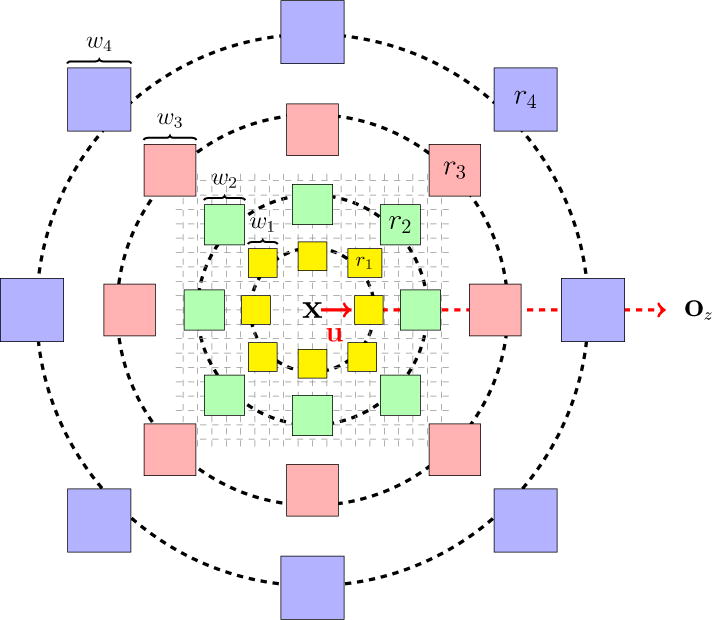
High resolution context descriptor. The voxel x at which this descriptor is calculated is at the center of this figure. The center of the slice o_z is shown on the right. The unit vector u is directed from x to o_z and is shown in red. It is rotated in increments of π/4 to identify the rest of the eight directions. At each radius ∈ {r₁, r₂, r₃, r₄}, along these eight different directions, we evaluate the mean of image intensities within a 3D cubic region (depicted here as colored 2D squares). The cubic widths {w₁, w₂, w₃, w₄} are also shown for a set of regions.

This yields a 32-dimensional descriptor of the context surrounding voxel x at the highest resolution. In our experiments, we have used the values w₁ = 3, w₂ = 5, w₃ = 7, w₄ = 9 and r₁ = 4, r₂ = 8, r₃ = 16, r₄ = 32, which were determined empirically. Since the head region is roughly spherical, this feature can disambiguate patches from different locations of the brain slice based on their near and far neighborhoods. We denote this feature vector as v(x). The feature vector at the finest level in the pyramid (s = 1) is the concatenated feature f¹(x) = [p¹(x), q¹(x), v(x)], which is used to train the final random forest regression stage to estimate the center voxel value $a_r^1\left(\mathbf{x}\right)$. Similar context descriptors have been independently formulated for segmentation tasks (Bai et al., 2015; Zikic et al., 2012).

2.2. Training a Random Forest

We train a random forest regressor RF_s at each level s to predict the voxel intensities in the target modality at that level from the feature vectors at that level (the orange, yellow, and green blocks in Fig. 1). A random forest regressor consists of an ensemble of regression trees (Breiman et al., 1984) with each regression tree partitioning the space of features into regions based on a split at each node in the tree. Let Θ_q = {[f₁; v₁],…, [f_t; v_t]} be the set of all training sample pairs at a node q in the tree. Here, f_i ∈ ℝ^J denotes the feature vector (which can be any one of those in the multi-resolution pyramid as described earlier) and v_i denotes a value in the modality to be predicted (which is the value of the image to be predicted at the same level in the multi-resolution pyramid). Let the mean of the target intensities of the samples at node q be ${\overline{v}}_q$. The nodal splits are determined during training by randomly selecting one third of the features (i.e., one third of the indices j = 1,…, J of the feature vector) and then finding the feature j in this subset together with a corresponding threshold τ_j that together minimize a least squares criterion as defined in the following paragraph.

The squared distance (SD) from the mean of the target intensities at node q is given by

$${\mathrm{SD}}_q={\displaystyle \sum _{i=1}^t{\left(v_i-{\overline{v}}_q\right)}^2}$$ (1)

where t is the number of training samples at node q. This quantity is seen as a measure of compactness of the target intensities in a node. Once feature j and threshold τ_j are selected to determine the split, as described below, then the training data are split into a “left” subset Θ_qL(j, τ_j) = {[f_i; v_i]|∀_i, f_ij≤τ_j} and a “right” subset Θ_qR(j, τ_j) = {[f_i; v_i]|∀_i, f_ij>τ_j}. These training samples are then used in new left and right child nodes in the tree. But how is the split determined? In fact, the split is made to make the left and right training data subsets as compact as possible. Given the split, each of these child nodes has its own compactness given by

$${\mathrm{SD}}_{qL}\left(j,{\tau }_j\right)={\displaystyle \sum _{i=1}^{t_L}{\left(v_i-{\overline{v}}_{qL}\right)}^2}$$ (2)

$${\mathrm{SD}}_{qR}\left(j,{\tau }_j\right)={\displaystyle \sum _{i=1}^{t_R}{\left(v_i-{\overline{v}}_{qR}\right)}^2},$$ (3)

where t_L and t_R are the number of samples in the left and the right child nodes, respectively, and the target intensities v_i are taken from their corresponding training samples. The compactness of the resulting training data can be maximized, if j and τ_j are chosen as

$$\left(\widehat{j},{\widehat{\tau }}_j\right)=\underset{j,{\tau }_j}{\arg min}{\mathrm{SD}}_{qL}\left(j,{\tau }_j\right)+{\mathrm{SD}}_{qR}\left(j,{\tau }_j\right).$$ (4)

This is the least squares criterion that determines node splits during training to create each random forest regressor.

The growth of each tree is controlled by three factors: t_p, t_c, and ɛ. If a node has fewer than t_p training samples, it will not be split into child nodes (and it therefore becomes a leaf node). If the optimum split of a given node leads to one of the child nodes having fewer than t_c training samples, then it will not be split (and it likewise becomes a leaf node). We set t_p = 2t_c and t_c = 5 in our experiments. If SD_q − (SD_qL + SD_qR) < ɛSD_q then the node is not split (and it likewise becomes a leaf node). We used ɛ = 10⁻⁶ in our experiments.

A master list of training data is created from the atlas data by sampling the features in all tissues making sure that abnormal tissues (like WMLs) are well-represented. Each RF regressor consists of sixty trees where each tree is learned from bootstrapped training data, where bootstrapping is carried out by randomly choosing N = 1 × 10⁵ training samples (with replacement) for each tree. Each trained tree contains the feature j and threshold τ_j at each non-leaf node and the average value of the target intensity at each leaf node. To use an RF regressor, the same feature vector is “fed” to each root node and each tree is traversed according to the stored feature indices and thresholds until a leaf node is reached whereupon the tree provides an intensity. The average intensity of all sixty trees is then formed as the output of the regressor.

2.3. Predicting a New Image

Given a subject image set, a Gaussian image pyramid is constructed and at each level s the subject image set is ${ℬ}^s=\{b_1^s,b_2^s,\dots ,b_m^s\}$ and relevant features are extracted. Starting from the coarsest level (s = S = 3 in all our experiments), RF_s is applied to synthesize the target modality at the lowest resolution ${\widehat{b}}_r^S$. This step is depicted in stage (d) of Fig. 1. For levels s < S, s ≠ 1, ${\widehat{b}}_r^S$ is upsampled to the next level to create ${\widehat{b}}_r^{S\uparrow }$, which is a synthetic, upsampled low resolution image. Feature vectors f^s(x) = [p^s(x), q^s(x)] are calculated at each voxel x at this level and RF_s is applied to these to generate ${\widehat{b}}_r^{S-1}$ (see stage (e) in Fig. 1). This process continues until s = 1. At s = 1, the highest available resolution, feature vectors f¹(x) = [p¹(x), q¹(x), v(x)] which includes the high resolution context descriptor v(x) are calculated. The trained random forest RF₁ is applied to produce the final high resolution synthetic image ${\widehat{b}}_r^1$ (stage (f) in Fig. 1).

We have provided a very general description of the REPLICA image synthesis pipeline. Depending on the complexity of the application we might use a subset of this pipeline. For example, when synthesizing images for which the input images are already skull-stripped, the intensity mapping does not need the entire multi-resolution treatment as the high resolution features are sufficient. REPLICA has a number of free parameters that can be tuned to improve the resulting synthesis. We performed extensive parameter selection experiments, the results of which are available in the Supplementary Materials. These parameters were set as follows, (a) number of trees (= 60), (b) number of samples in a leaf node (= 5), (c) size of local 3D patch (= 3 × 3 × 3), (d) number of individuals in the atlas (= 1), (e) use of alternate atlas images (does not affect synthesis), and (f) use of context and multi-resolution features, the results of which are shown in Section 3.2. For the remaining parameter selection experiments, please refer to the provided Supplementary Materials document.

3. Results

In Section 3.1 we describe results of synthesizing skull-stripped T₂w images using REPLICA. In Section 3.2 we describe results of synthesizing T₂w images that have not been skull-stripped. In Section 3.3 we demonstrate the use of REPLICA to synthesize FLAIR images, and finally in Section 3.4 we perform intensity standardization between SPGR and MPRAGE datasets using REPLICA.

3.1. Synthesis of T₂w Images

In this experiment, we synthesized T₂w images from skull-stripped T₁w MPRAGE images taken from the multimodal reproducibility resource (MMRR) data (Landman et al., 2011). The MMRR data consists of 21 subjects, each with two imaging sessions acquired within an hour of each other. T₂w images can be used as registration targets while performing distortion correction on echo-planar images (EPI) images and also as input to lesion segmentation algorithms. Therefore, if T₂w images are absent, we can use REPLICA to synthesize them. We compared REPLICA to the MIMECS method (Roy et al., 2013a) and a multi-atlas registration and intensity fusion method which we refer to as FUSION (Burgos et al., 2014). We used the NiftyReg affine and free-form deformation registration algorithm (Ourselin et al., 2001; Modat et al., 2010) and implemented the intensity fusion as described in Burgos et al. (2014). Burgos et al. use 40 atlases in their experiments with CT images. However, we have observed that using more than 20 atlases did not help in synthesizing abnormalities like lesions correctly. While in normal anatomy, the finer regions of the cortex get smoothed out due to fusion of more patches and are susceptible to mis-registration. Additionally, a large collection of appropriate paired atlas images is generally not available for most datasets. When atlas images are available, the registration+fusion for 20+ atlases can result in a run-time of 2 hours per synthetic image, which makes it unsuitable as a quick, preprocessing step.

We used data from one randomly chosen subject as training for REPLICA (the same subject was used in the parameter selection experiments described in the Supplementary Materials) and MIMECS and one image each from five subjects as the atlases for FUSION. We set the parameters for FUSION to β = 0.5 (weighting parameter) and κ = 4 (use the top 4 best patch matches to fuse); refer to Burgos et al. (2014) for more details. For the remaining 16 × 2 = 32 MPRAGE images, we synthesized T₂w images using all three methods. The input MPRAGE images were intensity standardized by scaling such that the white matter peak intensity in the histogram is 1. Synthesis of skull-stripped T₂w images can be achieved with an intensity transformation that is captured well using just the high resolution features. Therefore we do not use the entire multi-resolution framework for this application but only use the high resolution context descriptors and a local patch (f(x) = [p¹(x), v(x)]).

The atlas and subject images have the following specifications:

a1:	MPRAGE image (3 T, TR = 6.7 ms, TE = 3.1 ms, TI = 842 ms, 1.0 × 1.0 × 1.2 mm3 voxel size)
a2:	T2w image from the second echo of a DSE (3 T, TR = 6653 ms, TE1 = 30 ms, TE2 = 80 ms, 1.5 × 1.5 × 1.5 mm3 voxel size)
b1:	MPRAGE image (3 T, TR = 6.7 ms, TE = 3.1 ms, TI = 842 ms, 1.0 × 1.0 × 1.2 mm3 voxel size)

For evaluation of synthesis quality, we used PSNR (peak signal to noise ratio), which is a mean squared error-based metric, UQI (universal quality index) (Wang and Bovik, 2002), and SSIM (structural similarity) (Wang et al., 2004), with respect to the ground truth images. UQI and SSIM are more sensitive to perceptual differences in image structure than PSNR since they take into account properties of the human visual system. For both UQI and SSIM, a value of 1 indicates that the images are equal to each other; otherwise their values lie between 0 and 1. UQI and SSIM also quantify the differences in the luminance and contrast between the two images.

We can see from the results in Table 1 that REPLICA performs significantly better than the other methods for all metrics except PSNR. Figure 3 shows the results for all three methods along with the true T₂w image. FUSION ranks highest for PSNR, which can be explained by the fact that unlike the cortex, large, homogeneous regions of white matter have been reproduced quite well. However, it also produces anatomically incorrect images, especially in the presence of abnormal tissue anatomy (lesions for example) and the cortex (see Fig. 3(c)). MIMECS has a lower PSNR primarily due to boundary voxels, which are mostly skull voxels that were wrongly synthesized as CSF (see Fig. 3(d)). Overall, REPLICA produces an image that is visually closest to the true T₂w image and has the highest UQI and SSIM values.

Table 1.

Mean and standard deviation (Std. Dev.) of the PSNR, UQI, and SSIM values for synthesis of T₂w images from 32 MPRAGE scans by FUSION (multi-atlas registration + fusion), MIMECS (sparse dictionary reconstruction), and REPLICA (our approach)

	PSNR Mean (Std)	UQI Mean (Std.)	SSIM Mean (Std)
FUSION	52.73 (2.78)*	0.78 (0.02)	0.82 (0.02)
MIMECS	36.13 (2.23)	0.78 (0.02)	0.77 (0.02)
REPLICA	50.73 (2.67)	0.89 (0.02)*	0.87 (0.02)*

^*Statistically significantly better than either of the other two methods (p < 0.01) using a right-tailed test.

Figure 3.

Shown are (a) the input MPRAGE image, (b) the true T₂w image, and the synthesis results of (c) FUSION (Burgos et al., 2014), (d) MIMECS (Roy et al., 2013a), and (e) REPLICA (our method), followed by the corresponding difference images with respect to the true T₂w in (f), (g), and (h), respectively. The lesion (green arrow) and the cortex (orange arrow) in the true image are correctly synthesized by MIMECS and REPLICA, but not by FUSION. The dark boundary just outside the cerebral tissue (yellow arrow) is incorrectly synthesized as bright by MIMECS, but not by FUSION and REPLICA. The maximum intensity in the difference images is 224.25 whereas the maximum image intensity is 255.

3.2. Synthesis of Whole Head Images

Synthesis of whole head images, i.e. head images that are not skull-stripped, is challenging due to the presence of additional anatomical structures and the high variability of tissue intensities. Bone structures are typically dark on MRI and are adjacent to fat and skin, which are typically bright resulting in these regions having an extremely wide intensity range. The intensity transformation that needs to be learned is highly nonlinear and is generally one-to-many, especially if small patches are used as features. Small patches are useful if there are multiple input modalities capable of providing the necessary information to synthesize extra-cerebral tissues, as Roy et al. (2014) demonstrated by synthesizing CT images from input ultrashort echo time (UTE) images. The two UTE images together provide enough intensity information to differentiate the bone from soft tissues. But when these extra modalities are not available additional features are needed. Multi-resolution and context features, as described in Section 2.1, provide additional information about the location of a voxel within the brain, enabling better synthesis of these tissues. This experiment demonstrates the impact of these additional features. We use the T₁w MPRAGE images from the MMRR dataset (Landman et al., 2011) and synthesize corresponding full-head T₂w images. The input MPRAGE images were intensity standardized by scaling such that the white matter peak intensity in the histogram is 1. Data from one subject (the same data was used in the experiment described in Section 3.1) was used for training. The atlas and subject images have the same specifications as described in Section 3.1. REPLICA parameters were set as follows: number of trees= 60, and t_c = 5, t_p = 2t_c, and ɛ = 10⁻⁶.

We ran REPLICA with three different settings for input features: (a) only local 3 × 3 × 3 patches, (b) local patches + context features, and (c) local patches + context features + multi-resolution framework. Using each of these settings, we synthesized 20 × 2 = 40 synthetic images. Figure 4 shows a progression of REPLICA results for a synthetic T₂w image of a subject from the corresponding MPRAGE with both brain and non-brain tissues using a 3 × 3 × 3 local patch (Figs. 4(b) and 4(j)), a combination of the local patch and high resolution context descriptor (Figs. 4(c) and 4(k)), and the full REPLICA multi-resolution framework (Figs. 4(d) and 4(l)). Figures 4(f), 4(g), 4(h), 4(n), 4(o), and 4(p) also show the corresponding difference images with the ground truth T₂w image in Figs. 4(e) and 4(m). In this figure we show two slices, one from the inferior head region with a high variability of tissue intensities and structures, and another from a slightly superior region with more structured regions. This qualitative comparison reveals that the full multi-resolution framework works best.

Figure 4.

(a) Original input MPRAGE, (b) REPLICA T₂w synthesis using 3 × 3 × 3 patch as feature vector, (c) with additional high resolution context descriptor feature, and (d) using the full, multi-resolution REPLICA framework. (e) shows the ground truth T₂w image. In the next row we have the corresponding difference images with respect to the real T₂w image in (f), (g), and (h) respectively. It is clear that using multi-resolution REPLICA produces a higher quality synthesis for the challenging task of synthesis of full-head images. (i)–(p) Show the same images for a more superior slice. The maximum intensity in these images is 255. The difference images have a maximum intensity around 60.

For a quantitative comparison, we calculated PSNR, UQI, and SSIM from the 40 synthetic images to compare the effect of these feature settings. Box-plots for these metrics are shown in Fig. 5. These plots show quantitatively that the multi-resolution version of REPLICA is statistically significantly better (p < 0.01, one-tailed t-test) than the other two approaches in synthesizing T₂w images from MPRAGE images when the whole head is present.

Figure 5.

PSNR, UQI, and SSIM as functions of the features and multi-resolution framework of REPLICA.

Further, we provide a qualitative comparison of REPLICA against MIMECS and FUSION for this task (see Fig. 6). At first glance the FUSION result (Fig. 6(c)) looks appealing, but has errors in the cortical region which are similar to those found in the FUSION result in Section 3.1. MIMECS uses a small 3 × 3 × 3-sized patch and is unable to disambiguate between skull and CSF, resulting in large errors, especially in the ventricles (Fig. 6(d)). The REPLICA result (Fig. 6(e)) looks visually closer to the truth. It appears smoother in some regions due to dependence on low-resolution information coming from the lower levels of the multi-resolution framework.

Figure 6.

(a) The input MPRAGE image, (b) the real T₂w image, (c) FUSION result, (d) MIMECS result, (e) REPLICA result. Note the synthesis errors in the cortex for FUSION and in the ventricles for MIMECS.

3.3. Synthesis of FLAIR Images

In this experiment, we used REPLICA to synthesize a FLAIR image from T₁w, T₂w, and P_Dw images. The FLAIR pulse sequence is routinely used to image patients with multiple sclerosis (MS) and other diseases. It is particularly useful for visualization of white matter lesions (WML) which are observed in MS patients. White matter lesions appear hyperintense in FLAIR images and can be easily delineated using automated segmentation algorithms. The FLAIR sequence needs a long TI value and therefore, is generally acquired at a lower resolution for a faster scan time. FLAIR images also frequently suffer from artifacts, which result in hyperintensities that can be mistaken for lesions (Stuckey et al., 2007). Missing FLAIR images can also pose hurdles in lesion segmentation, as most leading lesion segmentation algorithms use FLAIR as an input modality (Shiee et al., 2010; Geremia et al., 2011; Llado et al., 2012). Synthesizing missing FLAIR images can help avoid these issues and enable segmentation and further image analysis.

The atlas set we used for this experiment is:

a1:	MPRAGE image (3 T, TR = 10.3 ms, TE = 6 ms, 0.82×0.82×1.17 mm3 voxel size)
a2:	T2w image from the second echo of a DSE (3 T, TR = 4177 ms, TE1 = 3.41 ms, TE2 = 80 ms, 0.82 × 0.82 × 2.2 mm3 voxel size)
a3:	PDw from the first echo of a DSE (3 T, TR = 4177 ms, TE1 = 3.41 ms, TE2 = 80 ms, 0.82 × 0.82 × 2.2 mm3 voxel size)
a4:	FLAIR (3 T, TI = 11000 ms, TE = 68 ms, 0.82 × 0.82 × 2.2 mm3 voxel size)

The subject image set is:

b1:	MPRAGE image (3 T, TR = 10.3 ms, TE = 6 ms,
b2:	T2w image from the second echo of a DSE (3 T, TR = 4177 ms, TE1 = 3.41 ms, TE2 = 80 ms, 0.82 × 0.82 × 2.2 mm3 voxel size)
b3:	PDw image from the first echo of a DSE (3 T, TR = 4177 ms, TE1 = 3.41 ms, TE2 = 80 ms, 0.82 × 0.82 × 2.2 mm3 voxel size)

All the modalities were registered and resampled to the MPRAGE image. All modalities were intensity standardized by scaling the intensities such that the white matter peak in each of the histograms was 1. This experiment did not need the multi-resolution framework as the image analysis takes place on skull-stripped images. We also tweaked the prediction of the decision trees in the random forest ensemble in this experiment. Instead of calculating the mean of the sample predictions in a single leaf, we calculated the mode. Calculating the mean resulted in oversmooth images, especially at the lesion-WM boundaries, which resulted in overestimation of lesion size by the segmentation algorithm. Using the mode results in crisper edges and better lesion segmentation. Input images along with the real and synthetic FLAIR images are shown in Fig. 7.

Figure 7.

Subject input images along with the synthetic and true FLAIR images.

We used our in-house MS patient image dataset with 125 images belonging to 84 subjects, with some subjects having images acquired longitudinally. We compared the synthesized images with existing true images using image similarity metrics (see Table 2). These values indicate that the synthetic FLAIR images are visually similar to the corresponding real FLAIR images. FLAIR synthesis results using FUSION (Figs. 8(b) and 8(f)), MIMECS (Figs. 8(c) and 8(g)) and REPLICA (Figs. 8(d) and 8(h)) for two different subjects can be compared visually with the corresponding real FLAIR images. FUSION was run with the same parameters as for the T₂w synthesis and it is unable to faithfully construct a synthetic image that is close enough to the ground truth. FUSION is based on registration and intensity fusion of multiple atlas images, and cannot synthesize lesion intensities at lesion locations if those intensities are not present in the atlas images at precisely those locations. We used only the T₁w images for the multi-atlas registration step in FUSION. Presence of lesions also affects the quality of the registrations itself, thus leading to a worse than expected result. MIMECS works better than FUSION but has errors synthesizing large lesion areas and very small lesions. Overall, REPLICA produces the most visually acceptable synthetic FLAIR image. We have not quantitatively compared REPLICA with MIMECS and FUSION on a large dataset because of the obvious and large errors in both of the MIMECS and FUSION results.

Table 2.

Mean (Std. Dev.) of PSNR (in decibels), UQI, and SSIM values over 125 FLAIR images synthesized by REPLICA.

PSNR	UQI	SSIM
21.73 (1.95)	0.84 (0.03)	0.81 (0.03)

Figure 8.

Visual comparison of FUSION, MIMECS and REPLICA for the FLAIR synthesis task. The two rows show images from different subjects. (a) and (e) real FLAIRs, (b) and (f) FUSION results, (c) and (g) MIMECS results, (d) and (h) REPLICA results.

Next, we used the synthetic FLAIR images as inputs to a tissue segmentation algorithm. If synthesis has been done correctly, the segmentation algorithm should behave similarly when either real or synthetic images are used as inputs. To test this, we used the LesionTOADS algorithm (Shiee et al., 2010). We compared the overlap of segmentations obtained using synthetic FLAIR images to those obtained using real FLAIR images in terms of Dice coefficients. The Dice coefficients for WM, GM, CSF, and WML classes are shown in Table 3. Figure 9 shows the segmentations by LesionTOADS on real and synthetic FLAIR images. The overlap is high for WM, GM, and CSF, however it is relatively low for the WML class. The lesions are small and diffuse and even a small difference in the overlap can cause a low value for the Dice coefficient (Geremia et al., 2011).

Table 3.

Mean (Std. Dev.) of Dice coefficients based on LesionTOADS segmentation of the real FLAIR and synthetic FLAIR over 125 images.

Algorithm	WM	GM	CSF	WML
LesionTOADS	0.97 (0.01)	0.99 (0.0005)	0.96 (0.01)	0.46 (0.22)

Figure 9.

(a) Original FLAIR, (b) synthetic FLAIR generated from T₁w, T₂w, and P_Dw images, (c) input MPRAGE for LesionTOADS segmentation, (d) LesionTOADS segmentation using real FLAIR + MPRAGE, (e) LesionTOADS segmentation using synthetic FLAIR + MPRAGE, and (f) a mask of segmentation differences between (d) and (e).

Thus we looked at the lesion volumes as provided by LesionTOADS for real and synthetic FLAIR images. To understand how different the lesion volumes are for the synthetic images as compared to the real images, we created a Bland-Altman plot (Bland and Altman, 1986) for these measurements (see Fig. 10). If y₁ and y₂ are two measurements by two different methods consisting of n samples each, then the Bland-Altman plot is a scatter plot of y₁ − y₂ versus (y₁ + y₂)/2. The measurements are considered to be interchangeable if 0 lies within ±1.96σ where σ is the standard deviation of y₁ − y₂. Figure 10 shows the Bland-Altman plot where y₁ are the lesion volumes for synthetic FLAIR images and y₂ are the lesion volumes for real FLAIR images, as produced, in both cases, by LesionTOADS. Even though the difference (y₁ − y₂) is not zero-mean (p > 0.05 using a one sample t-test), both the measurements can be used interchangeably because 0 lies within ±1.96σ in the plot (Bland and Altman, 1986).

Figure 10.

A Bland-Altman plot of lesion volumes for synthetic FLAIRs vs lesion volumes of real FLAIRs. Since zero lies within the ±1.96σ range, these two measurements of the same quantity are interchangeable.

3.4. Intensity Standardization

Tissue segmentation and cortical reconstruction in MRI are generally reliant on T₁w images acquired with sequences like MPRAGE, SPGR, etc. (Pham et al., 2000; Dale and Fischl, 1999; Van Leemput et al., 1999). However, most segmentation algorithms are not robust to variabilities in the T₁w image contrasts (Nyúl and Udupa, 1999). Intensity standardization of different contrasts has been proposed to alleviate this issue (Nyúl et al., 2000; Nyúl and Udupa, 1999; Jog et al., 2013b). Image synthesis can be used to standardize intensities by creating synthetic, standardized images from given images. These synthetic images can belong to a given, reference modality, on which the algorithm behavior is well-understood. We demonstrate such an intensity standardization application using the Baltimore Longitudinal Study of Aging (BLSA) dataset (Thambisetty et al., 2010). In this experiment, we used a subset of the dataset, consisting of 82 scans of 60 subjects, some of which are longitudinal acquisitions. Each scanning session was carried out on a Philips 1.5 T scanner and has an SPGR (see Fig. 11(a)) and an MPRAGE (see Fig. 11(c)) acquisition from the same session. We chose this dataset as it can mimic the scenario of a multi-site data acquisition where protocols differ across the sites. We use an in-house implementation of the probabilistic atlas-driven, EM-base segmentation algorithm by Van Leemput et al. (1999), which we refer to as AtlasEM. AtlasEM provides us with a 4-class segmentation, the classes being sulcal CSF, GM, WM, and ventricles. We segmented the SPGR and the MPRAGE images using AtlasEM. In an ideal scenario, where the algorithm is impartial to the underlying T₁w input, the segmentations should be identical. However, as we can observe in Figs. 11(d) and 11(f), the segmentations are quite different. We used REPLICA to generate a synthetic MPRAGE from input SPGR images, and ran AtlasEM segmentations on the synthetic MPRAGEs. The atlas set used for this experiment was:

Figure 11.

(a) SPGR, (b) synthetic MPRAGE, (c) real MPRAGE (d–f) their respective AtlasEM segmentations. The zoomed in location shows the segmentation differences in more detail.

a1:	SPGR image (1.5 T, TR = 35 ms, TE = 5 ms, α = 45°, 0.938 × 0.938 × 1.5 mm3 voxel size),
a2:	MPRAGE (1.5 T, TR = 6.92 ms, TE = 3.4 ms, α = 8°, 0.938 × 0.938 × 1.5 mm3 voxel size).

The subject images were:

b1:	SPGR image (1.5 T, TR = 35 ms, TE = 5 ms, α = 45°, 0.938 × 0.938 × 1.5 mm3 voxel size).

The synthesis did not need the multi-resolution framework as we work with skull-stripped images because the final segmentation takes place on skull-stripped Carass et al. (2011) images. We used the synthetic MPRAGE as an input for AtlasEM. Our goal is to show that the segmentations are now closer to those obtained by a real MPRAGE. Figure 11(b) shows the REPLICA-generated synthetic MPRAGE and Fig. 11(e) shows the segmentation for the same. Visually, it is closer to the segmentation obtained from the real MPRAGE Fig. (11(f)), especially at the CSF-GM interface.

We also looked at tissue volumes provided by AtlasEM on all three sets of images, SPGR, MPRAGE, and synthetic MPRAGE. As stated earlier, if the AtlasEM algorithm were robust to the input modality, the tissue volumes for a particular tissue should be identical for SPGR and MPRAGE. In Fig. 12, we show scatter plots for WM volumes obtained on real MPRAGEs (x-axis) and those obtained for SPGRs (blue) and synthetic MPRAGEs (red). We also show the least square line fits to the scatter plots (blue for SPGR, red for synthetic MPRAGE). In the ideal scenario, where the algorithm is indifferent to input contrast, the least square line fits should be close to the x = y line. We can see that for WM, synthetic MPRAGE volumes fit is closer to the identity line than SPGR volumes fit.

Figure 12.

AtlasEM WM volume scatter plots. The blue scatter plot is of volumes observed in SPGR versus those in MPRAGE. The red scatter plot is of volumes observed in synthetic MPRAGE versus those in MPRAGE. The black line indicates the identity transform x = y.

4. Discussion and Conclusions

We have described a new image synthesis algorithm called REPLICA. We have shown that REPLICA demonstrates significant improvement in image quality over other state-of-the-art synthesis algorithms (Section 3.1). We have also described applications where image synthesis in general and REPLICA in particular can be beneficial as a preprocessing step for subsequent image processing steps.

The T₂w synthesis for full-head images described in Section 3.2 also highlights the capability of REPLICA to handle complex image synthesis scenarios, with limited intensity information at its disposal. To our knowledge, REPLICA is the first intensity transformation-based synthesis approach to achieve this.

Synthesis of FLAIR images is a key application (Section 3.3) that has not been demonstrated before; this process can be useful if FLAIR images were not acquired, if the acquired FLAIR images are corrupted, or if higher-resolution FLAIR images are required. REPLICA is computationally fast. Training an ensemble can take up to 20 minutes, but needs to be done only once. With (easy) parallelization over eight cores, synthesis of a 256 × 256 × 173 image takes less than a minute on a 3 GHz computer. Given the typical times of neuroimaging pipelines (usually many hours), this makes the use of REPLICA as a preprocessing step quite feasible.

We have also shown use of REPLICA in intensity standardization applications where we have two imaging datasets with slightly different acquisition properties that produce different image processing results.

REPLICA has some limitations that should be addressed in the future. Since the predicted value of a random forest is the average of the results of all trees (each of which is an average of at least five values), the synthetic images often appear to have lower noise and be slightly smoother than their real counterparts. Lower noise may benefit algorithms but reduction in resolution is not typically beneficial. In a previous publication we have demonstrated super-resolution as an application of REPLICA (Jog et al., 2014b), so there may be a relatively straightforward way to enhance resolution in the exact amount needed to offset the inherent loss of resolution due to averaging. Also, we used the mode instead of the average in certain applications, but this is also an empirical strategy and not guaranteed to address the problem. Another limitation concerns the features that are used to train REPLICA. Although our features are sensible and effective for the applications we have explored, they are nevertheless empirically selected and they may not be optimal for these tasks or new scenarios that may be encountered in the future.

In our parameter selection experiments, despite improvements in image quality metrics with increasing patch size, in the experiments we used a 3 × 3 × 3 patch. Our rationale is as follows. First, we observed that improvements in our performance metrics from patch sizes 3 × 3 × 3 to 5 × 5 × 5 appear to be primarily due to noise reduction in large, homogeneous white matter regions. Such noise reduction yields synthetic images that are much smoother in appearance than real images. There is a concern that such images will not perform the same as real images in subsequent image processing. A second reason for using 3 × 3 × 3 patches is due to the increased computer memory burden (almost a factor of 3) of 5 × 5 × 5 patches. A third reason is that with the increase in feature dimensionality comes a requirement to increase the number of training samples and this puts a further memory burden on the software as well as a computation time increase. In particular, the training time goes from about 5 minutes to 40 minutes when going from 3 × 3 × 3 to 5 × 5 × 5 patches. Taking into consideration the concerns over unnatural noise reduction and the computational costs, we chose to use a 3 × 3 × 3-sized patch in all of our experiments. This parameter of REPLICA could be changed on a case-by-case basis to gain advantage in subsequent image processing steps due to noise reduction.

In conclusion, the REPLICA image synthesis method was described and shown to be effective in medical image processing tasks. REPLICA was shown to be beneficial when images are missing or corrupted for subsequent processing steps. It is a simple, fast, and effective approach that can be readily employed as a preprocessing step in many neuroimage processing pipelines.

Highlights.

• We describe an MRI image synthesis algorithm capable of synthesizing full-head T2w images and FLAIR images

• Our algorithm, REPLICA, is a supervised method and learns the nonlinear intensity mappings for synthesis using innovative features and a multi-resolution design

• We show significant improvement in synthetic image quality over state-of-the-art image synthesis algorithms

• We also demonstrate that image analysis tasks like segmentation perform similarly for real and REPLICA-generated synthetic images

• REPLICA is computationally very fast and can be easily used as a preprocessing tool before further image analysis

References

- Bahrami Khosro, Shi Feng, Zong Xiaopeng, Shin Hae Won, An Hongyu, Shen Dinggang. Medical Image Computing and Computer-Assisted Intervention – MICCAI 2015. Proceedings, Part II; 18th International Conference; Munich, Germany. October 5–9, 2015; Springer International Publishing; 2015. pp. 659–666. [DOI] [PMC free article] [PubMed] [Google Scholar]
- Bai W, Shi W, Ledig C, Rueckert D. Multi-atlas segmentation with augmented features for cardiac MR images. Medical Image Analysis. 2015;19:98–109. doi: 10.1016/j.media.2014.09.005. [DOI] [PubMed] [Google Scholar]
- Bland JM, Altman DG. Statistical methods for assessing agreement between two methods of clinical measurement. The Lancet. 1986;327:307–310. [PubMed] [Google Scholar]
- Breiman L. Bagging predictors. Machine Learning. 1996;24:123–140. [Google Scholar]
- Breiman L, Friedman JH, Olshen RA, Stone CJ. Classification and regression trees. Wadsworth Publishing Company; U.S.A.: 1984. [Google Scholar]
- Burgos N, Cardoso M, Thielemans K, Modat M, Pedemonte S, Dickson J, Barnes A, Ahmed R, Mahoney C, Schott J, Duncan J, Atkinson D, Arridge S, Hutton B, Ourselin S. Attenuation correction synthesis for hybrid PET-MR scanners: Application to brain studies. Medical Imaging, IEEE Transactions on. 2014;33:2332–2341. doi: 10.1109/TMI.2014.2340135. [DOI] [PubMed] [Google Scholar]
- Carass A, Cuzzocreo J, Wheeler MB, Bazin PL, Resnick SM, Prince JL. Simple paradigm for extra-cerebral tissue removal: Algorithm and analysis. NeuroImage. 2011;56:1982–1992. doi: 10.1016/j.neuroimage.2011.03.045. [DOI] [PMC free article] [PubMed] [Google Scholar]
- Cardoso MJ, Sudre CH, Modat M, Ourselin S. Template-based multimodal joint generative model of brain data. In: Ourselin S, Alexander DC, Westin CF, Cardoso MJ, editors. Information Processing in Medical Imaging. Springer International Publishing; 2015. pp. 17–29. [DOI] [PubMed] [Google Scholar]
- Dale AM, Fischl B. Cortical surface-based analysis: Segmentation and surface reconstruction. NeuroImage. 1999;9:179–194. doi: 10.1006/nimg.1998.0395. [DOI] [PubMed] [Google Scholar]
- Fonov V, Evans AC, Botteron K, Almli CR, McKinstry RC, Collins DL. Unbiased nonlinear average age-appropriate brain templates from birth to adulthood. NeuroImage. 2009;47(Supplement 1) Organization for Human Brain Mapping 2009 Annual Meeting. [Google Scholar]
- Fonov V, Evans AC, Botteron K, Almli CR, McKinstry RC, Collins DL. Unbiased average age-appropriate atlases for pediatric studies. NeuroImage. 2011;54:313–327. doi: 10.1016/j.neuroimage.2010.07.033. [DOI] [PMC free article] [PubMed] [Google Scholar]
- Geremia E, Clatz O, Menze BH, Konukoglu E, Criminisi A, Ayache N. Spatial decision forests for MS lesion segmentation in multi-channel magnetic resonance images. NeuroImage. 2011;57:378–390. doi: 10.1016/j.neuroimage.2011.03.080. [DOI] [PubMed] [Google Scholar]
- Han X, Pham DL, Tosun D, Rettman ME, Xu C, Prince JL. CRUISE: Cortical reconstruction using implicit surface evolution. NeuroImage. 2004;23:997–1012. doi: 10.1016/j.neuroimage.2004.06.043. [DOI] [PubMed] [Google Scholar]
- Hertzmann A, Jacobs CE, Oliver N, Curless B, Salesin DH. Proceedings of the 28th annual conference on Computer graphics and interactive techniques. 2001. Image analogies; pp. 327–340. [Google Scholar]
- Hor S, Moradi M. Scandent tree: A random forest learning method for incomplete multimodal datasets. In: Navab N, Hornegger J, W WM III, Frangi AF, editors. MICCAI. 1. Springer; 2015. pp. 694–701. [Google Scholar]
- Iglesias JE, Konukoglu E, Zikic D, Glocker B, Van Leemput K, Fischl B. 16th International Conference on Medical Image Computing and Computer Assisted Intervention (MICCAI 2013) Springer; Berlin Heidelberg: 2013. Is synthesizing MRI contrast useful for inter-modality analysis? pp. 631–638. [DOI] [PMC free article] [PubMed] [Google Scholar]
- Jog A, Carass A, Pham DL, Prince JL. 10th International Symposium on Biomedical Imaging (ISBI 2014) 2014a. Random forest FLAIR reconstruction from T1, T2, and PD-Weighted MRI; pp. 1079–1082. [DOI] [PMC free article] [PubMed] [Google Scholar]
- Jog A, Carass A, Pham DL, Prince JL. Tree-encoded conditional random fields for image synthesis. In: Ourselin S, Alexander DC, Westin CF, Cardoso MJ, editors. Information Processing in Medical Imaging. Springer International Publishing; 2015a. pp. 733–745. volume 9123 of Lecture Notes in Computer Science. [DOI] [PMC free article] [PubMed] [Google Scholar]
- Jog A, Carass A, Prince J. Biomedical Imaging (ISBI), 2014 IEEE 11th International Symposium on. 2014b. Improving magnetic resonance resolution with supervised learning; pp. 987–990. [DOI] [PMC free article] [PubMed] [Google Scholar]
- Jog A, Carass A, Roy S, Pham DL, Prince JL. MR image synthesis by contrast learning on neighborhood ensembles. Medical Image Analysis. 2015b;24:63–76. doi: 10.1016/j.media.2015.05.002. [DOI] [PMC free article] [PubMed] [Google Scholar]
- Jog A, Roy S, Carass A, Prince JL. 10th International Symposium on Biomedical Imaging (ISBI 2013) 2013a. Magnetic resonance image synthesis through patch regression; pp. 350–353. [DOI] [PMC free article] [PubMed] [Google Scholar]
- Jog A, Roy S, Carass A, Prince JL. Pulse sequence based multi-acquisition MR intensity normalization. Proceedings of SPIE Medical Imaging (SPIE-MI 2013); Orlando, FL. February 9–14 2013; 2013b. p. 86692H-86692H-8. [DOI] [PMC free article] [PubMed] [Google Scholar]
- Konukoglu E, van der Kouwe A, Sabuncu MR, Fischl B. 16th International Conference on Medical Image Computing and Computer Assisted Intervention (MICCAI 2013) Springer; Berlin Heidelberg: 2013. Example-based restoration of high-resolution magnetic resonance image acquisitions; pp. 131–138. [DOI] [PubMed] [Google Scholar]
- Landman BA, Huang AJ, Gifford A, Vikram DS, Lim IAL, Farrell JAD, Bogovic JA, Hua J, Chen M, Jarso S, Smith SA, Joel S, Mori S, Pekar JJ, Barker PB, Prince JL, van Zijl P. Multi-parametric neuroimaging reproducibility: A 3-T resource study. NeuroImage. 2011;54:2854–2866. doi: 10.1016/j.neuroimage.2010.11.047. [DOI] [PMC free article] [PubMed] [Google Scholar]
- Llado X, Oliver A, Cabezas M, Freixenet J, Vilanova JC, Quiles A, Valls L, Ramio-Torrent L, Rovira A. Segmentation of multiple sclerosis lesions in brain MRI: A review of automated approaches. Information Sciences. 2012;186:164–185. [Google Scholar]
- Miller MI, Christensen GE, Amit Y, Grenander U. Mathematical textbook of deformable neuroanatomies. Proc Natl Acad Sci. 1993;90:11944–11948. doi: 10.1073/pnas.90.24.11944. [DOI] [PMC free article] [PubMed] [Google Scholar]
- Modat M, Ridgway GR, Taylor ZA, Lehmann M, Barnes J, Hawkes DJ, Fox NC, Ourselin S. Fast free-form deformation using graphics processing units. Computer Methods and Programs in Biomedicine. 2010;98:278–284. doi: 10.1016/j.cmpb.2009.09.002. HP-MICCAI 2008. [DOI] [PubMed] [Google Scholar]
- Nyúl LG, Udupa JK. On standardizing the MR image intensity scale. Mag Reson Med. 1999;42:1072–1081. doi: 10.1002/(sici)1522-2594(199912)42:6<1072::aid-mrm11>3.0.co;2-m. [DOI] [PubMed] [Google Scholar]
- Nyúl LG, Udupa JK, Zhang X. New variants of a method of MRI scale standardization. IEEE Trans Med Imag. 2000;19:143–150. doi: 10.1109/42.836373. [DOI] [PubMed] [Google Scholar]
- Ourselin S, Roche A, Subsol G, Pennec X, Ayache N. Reconstructing a 3D structure from serial histological sections. Image and Vision Computing. 2001;19:25–31. [Google Scholar]
- Pham DL, Xu C, Prince JL. Current methods in medical image segmentation. Annual Review of Biomedical Engineering. 2000;2:315–337. doi: 10.1146/annurev.bioeng.2.1.315. [DOI] [PubMed] [Google Scholar]
- Prastawa M, Gilmore J, Lin W, Gerig G. 7th International Conference on Medical Image Computing and Computer Assisted Intervention (MICCAI 2004) Springer; Berlin Heidelberg: 2004. Automatic segmentation of neonatal brain MRI; pp. 10–17. [Google Scholar]
- Roohi S, Zamani J, Noorhosseini M, Rahmati M. Electrical Engineering (ICEE), 2012 20th Iranian Conference on. 2012. Super-resolution MRI images using compressive sensing; pp. 1618–1622. [Google Scholar]
- Rousseau F. 2008 European Conference on Computer Vision (ECCV 2008) 2008. Brain Hallucination; pp. 497–508. [Google Scholar]
- Rousseau F. A non-local approach for image super-resolution using intermodality priors. Medical Image Analysis. 2010;14:594–605. doi: 10.1016/j.media.2010.04.005. [DOI] [PMC free article] [PubMed] [Google Scholar]
- Rousseau F, Studholme C. 10th International Symposium on Biomedical Imaging (ISBI 2013) 2013. A supervised patch-based image reconstruction technique: Apllication to brain MRI super-resolution; pp. 346–349. [Google Scholar]
- Roy S, Carass A, Bazin PL, Resnick SM, Prince JL. Consistent segmentation using a Rician classifier. Medical Image Analysis. 2012;16:524–535. doi: 10.1016/j.media.2011.12.001. [DOI] [PMC free article] [PubMed] [Google Scholar]
- Roy S, Carass A, Prince JL. Synthesizing mr contrast and resolution through a patch matching technique. Proceedings-Society of Photo-Optical Instrumentation Engineers. 2010a;7623:76230j. doi: 10.1117/12.844575. [DOI] [PMC free article] [PubMed] [Google Scholar]
- Roy S, Carass A, Prince JL. 22nd Inf Proc in Med Imaging (IPMI 2011) 2011. A compressed sensing approach for MR tissue contrast synthesis; pp. 371–383. [DOI] [PMC free article] [PubMed] [Google Scholar]
- Roy S, Carass A, Prince JL. Magnetic resonance image example-based contrast synthesis. Medical Imaging, IEEE Transactions on. 2013a;32:2348–2363. doi: 10.1109/TMI.2013.2282126. [DOI] [PMC free article] [PubMed] [Google Scholar]
- Roy S, Carass A, Shiee N, Pham DL, Prince JL. 7th International Symposium on Biomedical Imaging (ISBI 2010) 2010b. MR contrast synthesis for lesion segmentation; pp. 932–935. [DOI] [PMC free article] [PubMed] [Google Scholar]
- Roy S, Jog A, Carass A, Prince JL. 3rd International Workshop on Multimodal Brain Image Analysis at the 16th International Conference on Medical Image Computing and Computer Assisted Intervention (MICCAI 2013) 2013b. Atlas based intensity transformation of brain MR images; pp. 51–62. [Google Scholar]
- Roy S, Wang WT, Carass A, Prince JL, Butman JA, Pham DL. PET attenuation correction using synthetic CT from ultrashort echo-time MR imaging. Journal of Nuclear Medicine. 2014;55:2071–2077. doi: 10.2967/jnumed.114.143958. [DOI] [PMC free article] [PubMed] [Google Scholar]
- Shiee N, Bazin PL, Cuzzocreo JL, Ye C, Kishore B, Carass A, Calabresi PA, Reich DS, Prince JL, Pham DL. Robust reconstruction of the human brain cortex in the presence of the WM lesions: Method and validation. Human Brain Mapping. 2014;35:3385–3401. doi: 10.1002/hbm.22409. [DOI] [PMC free article] [PubMed] [Google Scholar]
- Shiee N, Bazin PL, Ozturk A, Reich DS, Calabresi PA, Pham DL. A topology-preserving approach to the segmentation of brain images with multiple sclerosis lesions. NeuroImage. 2010;49:1524–1535. doi: 10.1016/j.neuroimage.2009.09.005. [DOI] [PMC free article] [PubMed] [Google Scholar]
- Stuckey S, Goh TD, Heffernan T, Rowan D. Hyperintensity in the subarachnoid space on FLAIR MRI. American Journal of Roentgenology. 2007;189:913–921. doi: 10.2214/AJR.07.2424. [DOI] [PubMed] [Google Scholar]
- Thambisetty M, Wan J, Carass A, An Y, Prince JL, Resnick SM. Longitudinal changes in cortical thickness associated with normal aging. NeuroImage. 2010;52:1215–1223. doi: 10.1016/j.neuroimage.2010.04.258. [DOI] [PMC free article] [PubMed] [Google Scholar]
- van Tulder G, de Bruijne M. Why does synthesized data improve multi-sequence classification? In: Navab N, Hornegger J, Wells W, Frangi A, editors. 18th International Conference on Medical Image Computing and Computer Assisted Intervention (MICCAI 2015) Springer International Publishing; 2015. pp. 531–538. [Google Scholar]
- Van Leemput K, Maes F, Vandermeulen D, Suetens P. Automated model-based tissue classification of MR images of the brain. Medical Imaging, IEEE Transactions on. 1999;18:897–908. doi: 10.1109/42.811270. [DOI] [PubMed] [Google Scholar]
- Van Nguyen H, Zhou K, Vemulapalli R. Cross-Domain Synthesis of Medical Images Using Efficient Location-Sensitive Deep Network. In: Navab N, Hornegger J, Wells W, Frangi AF, editors. 18th International Conference on Medical Image Computing and Computer Assisted Intervention (MICCAI 2015) Springer International Publishing; 2015. pp. 677–684. [Google Scholar]
- Wang Z, Bovik AC. A universal image quality index. IEEE Signal Proc Letters. 2002;9:81–84. [Google Scholar]
- Wang Z, Bovik AC, Sheikh HR, Member S, Simoncelli EP. Image quality assessment: From error visibility to structural similarity. IEEE Trans Image Proc. 2004;13:600–612. doi: 10.1109/tip.2003.819861. [DOI] [PubMed] [Google Scholar]
- Ye DH, Zikic D, Glocker B, Criminisi A, Konukoglu E. 16th International Conference on Medical Image Computing and Computer Assisted Intervention (MICCAI 2013) Springer; Berlin Heidelberg: 2013. Modality propagation: Coherent synthesis of subject-specific scans with data-driven regularization; pp. 606–613. [DOI] [PubMed] [Google Scholar]
- Zikic D, Glocker B, Criminisi A. Encoding atlases by randomized classification forests for efficient multi-atlas label propagation. Medical Image Analysis. 2014;18:1262–1273. doi: 10.1016/j.media.2014.06.010. [DOI] [PubMed] [Google Scholar]
- Zikic D, Glocker B, Konukoglu E, Shotton J, Criminisi A, Ye D, Demiralp C, Thomas OM, Das T, Jena R, Price SJ. Context-sensitive classification forests for segmentation of brain tumor tissues. MICCAI 2012 Challenge on Multimodal Brain Tumor Segmentation. 2012 URL: http://research.microsoft.com/apps/pubs/default.aspx?id=172241.
Associated Data
This section collects any data citations, data availability statements, or supplementary materials included in this article.