Optics of high-performance electron microscopes

Abstract

During recent years, the theory of charged particle optics together with advances in fabrication tolerances and experimental techniques has lead to very significant advances in high-performance electron microscopes. Here, we will describe which theoretical tools, inventions and designs have driven this development. We cover the basic theory of higher-order electron optics and of image formation in electron microscopes. This leads to a description of different methods to correct aberrations by multipole fields and to a discussion of the most advanced design that take advantage of these techniques. The theory of electron mirrors is developed and it is shown how this can be used to correct aberrations and to design energy filters. Finally, different types of energy filters are described.

Introduction

The resolution of any imaging microscope is ultimately limited by the wavelength of the image-forming wave. About 1870, Ernst Abbe found this insight while trying to improve the resolution limit of light microscopes. In a visionary statement, he argued that there might be some yet unknown radiation with a shorter wavelength than that of light enabling a higher resolution at some time in the future. The discoveries of x-rays and electron rays provided such radiation. Unfortunately, proper lenses for x-rays do not exist. However, each rotationally symmetric electromagnetic field acts in paraxial approximation as a focusing lens for charged particles, electrons in particular. Moreover, the wavelength of electrons Å is significantly smaller than that of light, even at very small energies E, m is the mass of the electron. The resolution limit of conventional electron microscopes is about thousand times smaller than that of the best light microscopes. Therefore, it can visualize objects, which are so small that they are by no means accessible in light microscopy. The invention of the electron microscope has been one of the most important achievements of the last century owing to its impact on materials science, biology, virology and medicine, to name only a few. For example, most viruses are so small that they can only be visualized in the electron microscope.

Electron microscopy is based on two fundamental discoveries, one made in 1924 by Louis de Broglie [1], the other in 1926 by Hans Busch [2]. De Broglie postulated on ground of theoretical considerations that a wave must be associated to each elementary particle. At about the same time Busch discovered that the magnetic field of a solenoid acts on electrons in the same way as a convex glass lens acts on light rays. It had been these two important discoveries which lead Ernst Ruska to the conclusion that it must be possible to build a microscope which uses electrons instead of photons. He realized successfully the first electron microscope in 1931. For more than 40 years all transmission electron microscopes were based on Ruska's design [3]. During this period of time the resolution increased primarily due to improvements in the stability of the column, the specimen stage, the lens currents and owing to better shielding of parasitic external electromagnetic fields.

In order to fully exploit the capabilities of electron microscopes, it was necessary to develop it from an instrument producing merely pictures to an analytical instrument yielding quantitative information about the structure, the chemical composition and the electronic properties of the object on an atomic scale. The first step toward this goal was made by A. Crewe and coworkers [4] about 30 years ago with the construction of the scanning transmission electron microscope (STEM). This instrument is equipped with a field emission gun and a spectrometer which enables, at least in principle, the recording of the energy-loss spectrum parallel with the image formed by the elastically scattered electrons. This procedure produces the three-dimensional ‘information cube’ shown in figure 1. Somewhat later Zeiss incorporated the Henry–Castaing imaging energy filter [5] in the transmission electron microscope (TEM) primarily to remove the inelastically scattered electrons from the image-forming electron beam. However, since the STEM had demonstrated that these electrons contain valuable information on the chemical composition and the bonding states of the specimen, improved in-column imaging energy filters were designed, built and incorporated in the TEM [6]. These filters are optimally placed in front of the projector lenses. To convert conventional TEMs retroactively into energy-filtering TEMs (EFTEM), an attachable post-column imaging energy filter was developed by the manufacturer Gatan. The EFTEM produces the three-dimensional information cube consisting of an energy-loss spectrum for each image point by taking images with different energy windows, while the STEM achieves this by recording the energy-loss spectrum for each picture element (pixel). The TEM images all object points in parallel, while all scanning electron microscopes (SEM) form the image sequentially, as illustrated in figure 1. Most SEMs use voltages between 10 and 60 kV. The high-resolution STEMs operate at higher voltages between 100 and 300 kV. The SEM records the image with the signal of either the secondary electrons or the backscattered electrons, whereas the STEM utilizes the transmitted scattered electrons.

Figure 1.

The information cube consisting of an energy-loss spectrum for each image point.

Unfortunately, the performance of rotationally symmetric electron lenses is rather poor because they suffer from large unavoidable spherical and chromatic defects. This is known as the Scherzer theorem [7]. The reason for this behavior is due to the fact that the electromagnetic potentials satisfy Laplace's equation in the domain of the particles. As a result, the spatial distribution of the index of refraction of electron lenses cannot be formed arbitrarily. Since the potential adopts an extremum at the boundaries, the outer zones of rotationally symmetric electron lenses always focus the rays more strongly than the inner zones, causing spherical aberration. Chromatic aberration arises because electrons whose velocities differ from those with nominal velocity are diffracted differently, the slower electrons more strongly than the faster ones. Owing to these aberrations, the resolution limit of uncorrected electron microscopes is about 100 times the wavelength of the image forming electrons, whereas this limit is somewhat smaller than the wavelength in the best diffraction-limited light microscopes. To avoid radiation damage caused by atom displacements, the energy of the electrons must be smaller than the threshold energy for knock-on processes, which lies in the region between 100 and 300 keV for most solid materials. Therefore, it is generally not possible to increase the resolution (inverse of the resolution limit) by shortening the wavelength of the electrons without severely damaging the object. The resolution limit of an uncorrected 200 kV TEM is about 2 Å which does not suffice to resolve the atomic structure of non-periodic object details such as interfaces, stacking faults, grain boundaries and amorphous nano-clusters. However, these microscopic defects largely determine the macroscopic properties of solid objects, and are therefore very important. This is the major reason for the ongoing struggle to eliminate the resolution-limiting aberrations of electron microscopes. In recent years multipole correctors have been designed and built which compensate for the spherical aberration of round lenses. By means of these correctors Haider et al [8] and Krivanek et al [9] achieved a resolution limit of about 1 Å in the TEM and the STEM, respectively. In order to enable local spectroscopy with an energy resolution of about 0.1 eV, it is necessary that the energy width of the incident electron beam is smaller than this value. Since most electron sources have a significantly larger energy spread, monochromators are needed. A monochromator reduces the energy width of the incident electron beam by removing all electrons whose energy deviation exceeds a given limit. Recently Kahl et al [10, 11] have designed and successfully realized a suitable electrostatic monochromator, which reduces the energy spread of the beam to about 0.1 eV without affecting the coherence properties of the illumination. The incorporation of the monochromator, the aberration corrector, and a highly dispersive aberration-free imaging energy filter will enable sub-eV energy resolution and sub-angstrom spatial resolution in future high-performance analytical TEMs. As of 2004, the development of such a sub-angstrom TEM aiming for a resolution limit of about 0.8 Å at 200 kV is pursued by the SATEM project in Germany. The realization of an equivalent instrument with a resolution limit of about 0.5 Å is the task of the ambitious TEAM project in the USA. For achieving the latter resolution and for efficiently utilizing the inelastically scattered electrons, it is necessary to correct both the spherical aberration and the chromatic aberration by means of a sophisticated electric and magnetic quadrupole–octopole corrector consisting of at least 12 elements [11, 12]. The primary chromatic aberration is proportional to the relative energy spread ΔE/E of the image-forming electrons, where E=eU is the nominal energy. Since this aberration increases with decreasing acceleration voltage U, chromatic and spherical aberration of uncorrected round lenses are roughly equal at voltages of about 10 kV. Hence, in order to appreciably improve the resolution at low voltages, we must eliminate or reduce sufficiently both aberrations. An actual reduction of the resolution limit by a factor of about three was first achieved by Zach and Haider [13] in 1995 for a low-voltage scanning electron microscope (LVSEM) by means of a corrector consisting of a proper combination of electrostatic and magnetic quadrupoles and octopoles. Unfortunately, this corrector cannot be used for imaging extended object areas in a TEM owing to the large field (off-axial) aberrations of this corrector. These aberrations stay sufficiently small for the mirror corrector, which allows the transfer of large object fields [14]. By employing this corrector, it is possible to push the resolution limit of low-voltage electron microscopes (LEEM) and photo-emission electron microscopes (PEEM) down to about 1 nm for electrons with very low starting energies at the object. Mirror-corrected PEEMs will be installed at the Berlin Electron Synchrotron (BESSY 2) and the Advanced Light Source (ALS) at the Lawrence Berkeley National Laboratory in the near future.

The design of the novel components for the new generation of aberration-corrected analytical electron microscopes has been possible only due to the advancements made in electron optics during the last 20 years. This article outlines the present state of this development.

To describe the properties of electron optical elements and systems, it is extremely useful to employ the concepts, notations and nomenclature of light optics. The light-optical principles and mathematical methods have been proved invaluable for designing optimum aberration correctors, monochromators and imaging energy filters, despite the fact that these components consist of non-rotationally symmetric elements such as dipoles, quadrupoles and higher-order multipoles.

The main task of charged-particle optics in microscopy is the manipulation of ensembles of rays, each originating from a distinct object point. An important collective property of optical elements is, for example, the focusing of these homocentric bundles of rays forming a point-to-point image. Another example is the guiding of particles in accelerators or storage rings. We will mainly be concerned with these aspects of charged-particle optics. Methods for producing charged particles will not be described here.

Fundamentals of particle optics

Geometric charged-particle optics describes the motion of charged particles in macroscopic electromagnetic fields by employing the well-established notations and concepts of light optics. Macroscopic fields are produced by macroscopic elements, such as solenoids, magnetic multipoles or by voltages applied to conducting devices, for example cylinders or apertures. The atomic fields within solid or biological objects are defined as microscopic fields. The propagation of the particles in these fields is usually not be considered within the frame of charged-particle optics.

The description of the particle motion from the point of view of light optics is reasonable because the elementary particles have particle and wave properties. Moreover, the properties of particle-optical instruments and their constituent components are described most appropriately in light-optical terms which have been established at a time when charged particles were still unknown. The treatment of particle motion by means of optical concepts has been proven extremely useful for the design of beam-guiding systems, the electron microscope in particular. Since the invention in 1931, the electron microscope has developed over the years from an image-forming system to a sophisticated analytical instrument yielding structural and chemical information on an atomic scale.

The influence of diffraction on the particle quantum wave becomes negligibly small in the limit that the refraction index does not change significantly over the distance of several wavelength. This limit represents the domain of geometrical particle optics. The effect of the spin on the motion of charged particle is of the same order of magnitude as that resulting from diffraction. Electrons and ions are described by the same formalism because their propagation in macroscopic fields depends only on their mass and charge.

For reasons of simplicity we restrict our further investigations to electrons. Nevertheless, all results can be used for ions as well if we substitute their charge and rest mass for the corresponding quantities of the electron. Geometrical light optics describes the properties of optical elements by means of their effects on the light rays along which photons propagate. The rays form straight lines in the region outside the lenses. These rays are either refracted at the surfaces of the lenses where the index of refraction changes abruptly, or are deflected steadily if the index of refraction changes gradually, as for example in gradient-index lenses where the index of refraction increases quadratic with the distance from their optic axis. In close analogy, geometrical electron optics conceives the path of an electron as a geometrical line or trajectory. However, contrary to light optics, all electron optical elements form gradient-index lenses because the electrons must travel in vacuum where the electromagnetic fields produced by the exterior currents and charges vary continuously.

Variational principles

The path taken by a charged particle is governed by the Lorentz equation , where it can be derived from a variational principles. It was first shown by Hamilton that the optical laws can be obtained from a single characteristic function which was later called eikonal, derived from the Greek word ∊ικoν meaning image. Hamilton himself showed that the techniques he had developed for handling optical problems are also applicable in mechanics. This is the reason that many problems of charged-particle optics are most effectively treated by means of the eikonal method. This function is obtained most conveniently by employing Hamilton's principle, or the Lagrange variational principle.

Lagrange variational principle

The well-known Lagrange variational principle requires

with the Lagrangian , Hamiltonian , and canonical momenta and coordinates .

In this principle all variations of are allowed and therefore the Euler–Lagrange equations of motion hold,

For relativistic single-particle motion, the Lagrangian is

where the position is a function of the coordinates . The Jacobian matrix r of this function can be written in the form and has the elements r_ij=∂_qjr_i. In this efficient notation is the transpose of the 3×1 matrix . The Jacobian matrix of the function is also r since .

The canonical momentum is and the variational principle can thus be written as

Maupertuis principle

The variational principle for constant total energy is called the principle of Maupertuis. Here only variations are considered which keep the total energy constant, so that the variational principle becomes

However, equation (5) does not lead directly to Euler–Lagrange equations of motion, since not all variations are allowed.

A particle optical device usually has an optic axis or some design curve along which a central particle of the beam should travel. This design curve is parameterized by the arc length z and the position of a particle in the vicinity of the design curve has coordinates x and y along the unit vectors and in a plane perpendicular to this curve. This coordinate system is shown in figure 2. The third coordinate vector is tangential to the design curve and the curvature vector is .

Figure 2.

Curvatures κ_x, κ_y of the design curve and coordinates x, y and z.

The unit vectors in the usual Frenet–Serret comoving coordinate system rotate with the torsion of the design curve. If this rotation is wound back, the equations of motion do not contain the torsion of the design curve and . The position and the velocity are then

with h=1+xκ_x+yκ_y. This method is described in [15, 16] and is mentioned here since design curves with torsion are becoming important when considering particle motion in helical wigglers, undulators and wavelength shifters [17], and for polarized particle motion in helical dipole Siberian Snakes [18].

The variational principle in equation (5) for the three coordinates x(t), y(t) and z(t) can now be written for the two coordinates x(z) and y(z). This has the following two advantages: (a) the particle trajectory along the design curve is usually more important than the particle position at a time t, and (b) whereas does not allow for all variations of the three coordinates, the total energy can be conserved for all variations of the two coordinates x and y by choosing for each position the appropriate momentum with . We obtain from equation (5)

with and . Since all variations are allowed, the integrand is a very simple new Lagrangian

which leads to Euler–Lagrange equations of motion

The eikonals of particle optics

The integral over for a physical trajectory for which it is extremal, i.e. along which holds, is called the eikonal and is written as . It can be computed with equation (7) by where the physical path has to be chosen that connecting the initial coordinates and the final coordinates . It therefore is a function of the initial and final coordinates and the eikonal can therefore be written as

The Maupertuis principle can now be written as . The variation of coordinates at the final point leads to . The direction of the particle trajectories is therefore perpendicular to the surfaces of constant eikaonl is there is no vector potential. Otherwise the canonical momentum is perpendicular to those surfaces. This description is illustrated in figure 3. Extremal fields influence the trajectories by deforming these surfaces.

Figure 3.

Path of the electron as orthogonal trajectories of the set of surfaces of constant reduced action in the case .

The eikonal depending on the initial and final positions is also called the point eikonal. There are also other eikonals which are produced by Lagandre transformations. The mixed eikonal , where the final position has to be expressed as a function of and . The final position can then be computed by

Here, it becomes clear that the eikonals are generating functions of the canonical transformation between initial and final phase space coordinates [19].

The index of refraction n, which is well known for light optics, can be generalized to particle optics. This generalizes Fermat's principle to a principle of least action.

Fermat principle

Maupertuis variational principle of particle motion is analogous to Fermat's principle of light propagation. According to this principle, a light path leads to an extremum:

where is the optical index of refraction at position . Due to the similarity with equation (9), one defines the index of refraction of charged-particle optics as .

Image formation in the electron microscope

Paraxial optics

A plane in which the all paraxial rays originating in the center of the object plane join in a single point is called an image plane. The optics between these two planes is then said to be point to point imaging.

A plane in which all fundamental rays originating in the object plane with the same slope are imaged to a point is called the diffraction plane. The optics between these two planes is then said to be parallel to point imaging.

Fundamental paraxial rays

Particle-optical systems are usually designed so that the paraxial trajectories represent the ideal particle rays. Unfortunately, this course of the rays can never be achieved in a real system owing to the unavoidable nonlinear terms in the equation of motion. However, it may be possible to eliminate the deviations of the true path from its paraxial approximation at a distinct plane by properly adjusting the distribution of the electromagnetic field in the space between this plane and the initial plane. The problem of determining the optimum field distribution is extremely complicated and has not yet fully been solved. Without an insight into the properties of the path deviations it is almost impossible to find a suitable correction method for the resolution-limiting aberrations.

It is therefore useful to introduce fundamental paraxial rays which satisfy the linearized equation of motion, which can for example be computed by the second-order expansion of the eikonal in equation (9).

Theorem of alternating images

Within a multi-stage system, such as the electron microscope, each plane will be imaged repeatedly. As an example, we consider the formation of the images of two planes A and C located as depicted in figure 4. Typical locations are the object plane and the back focal plane of a lens. This plane is an image plane of the source for parallel illumination. We center an aperture at each of the two planes. As the pair of linearly independent trajectories, we select the fundamental rays

where u_α and u_γ intersect the optic axis at the center of the aperture A and C, respectively. The aperture A is imaged in the planes z_αn and the aperture C in the planes z_γn. In linear approximation, the position u and the transverse momentum conserve the Wronskian:

Figure 4.

Illustration of the theorem of alternating images.

Since u_α(z_αn)=u_α(z_αm)=0, the slopes of u_α at the planes z_αn and z_αm must have opposite sign, as demonstrated in figure 4. Considering this behavior, it readily follows that u_γ must change its sign in the region between two subsequent images of the aperture A. This is only possible if an image of the aperture C, i.e. u_γ(z_γn)=0, is located in this domain. Accordingly, we can state: an optical system always forms an image of the source in the domain between any two subsequent images of the object plane.

Figure 5 illustrates the consequences of this theorem for the image formation in an ideal electron microscope. The crossover of the cathode forms the effective source, which is formed at some distance from the surface of the emitter. For a field emission gun, the crossover is generally virtual and located inside the tip of the emitter. The condenser system adjusts the illumination of the object. In order to achieve an ideal illumination system, the condenser should consist of two lenses and two apertures, one placed at the image of the crossover, the other at an image of the cathode surface. The former aperture is imaged in the object plane and limits the field of illumination, whereas the second aperture determines the maximum angle of illumination. A special kind of this illumination is known from light optics as ‘Koehler illumination', which is assumed in figure 5. This illumination images the surface of the cathode in the back focal plane of the objective lens, and has the advantage that local variations of the electron emission on the cathode surface do not show up as artifacts in the image of the object. The location of the crossover image can be varied by changing the illumination mode.

Figure 5.

Scheme of the path of the fundamental paraxial trajectories and location of the images and heam-limiting apertures in a transmission electron microscope illustrating the theorem of alternating images.

For Koehler illumination, the back focal plane of the objective lens is also the diffraction plane of the object. In accordance with the famous optician E Abbe, one defines the diffraction pattern at this plane as the ‘primary image’. Owing to the spherical aberration of the objective lens, the large-angle scattered electrons miss the Gaussian image point and blur the image. In order to remove these electrons from the beam, one places an objective aperture at the back focal plane of this lens. Each intermediate image of the object is also an image of the illumination-field aperture, and each image of the illumination-angle aperture coincides with that of the objective aperture. The special locations of the two illumination apertures allow one to vary the illuminated area in the object plane without affecting the angular illumination and vice versa. The characteristic planes in an electron microscope are, therefore, real and virtual images of the object plane and the crossover plane or those of the two illumination apertures, respectively. It is impossible to form two subsequent images of one of these two planes without having an image of the other plane located between them.

Correction of aberrations

Abbe's sine condition

The spherical aberration of the objective lens determines the resolution and the off-axial coma the field of view of the recorded image. The projector lenses introduce primarily distortion. Hence, to obtain ideal imaging, we must compensate for the spherical aberration and the coma of the objective lens and for the distortion of the projector system. We eliminate the distortion by properly exciting the constituent lenses of the projector system. Unfortunately, this is not possible for the spherical aberration due to the Scherzer theorem. Imaging systems which are free of spherical aberration and coma are called aplanats. These systems satisfy the sine condition, as demonstrated by Abbe [20]. The sine condition gives information about the quality of the image at off-axial points in terms of the properties of the pencil of axial rays.

Here denotes the lateral component of the canonical momentum. The gauge of the magnetic vector potential is chosen as

which guarantees that the canonical momentum of the particle coincides with its kinetic momentum at any point along the optic axis. The mixed eikonal V is a function of the four variables x_o, y_o, p_xi and p_yi, and of the locations z_o and z_i of the object plane and of the image plane, respectively. For mathematical simplicity, we express the two-dimensional vectors , and by the complex quantities

The corresponding conjugate complex quantities are indicated by a bar. Since the variation δV vanishes for fixed w_o and p_i, the lateral component of the canonical momentum p_o at the object plane and the off-axial position of the trajectory at the image plane z_i can be obtained from the eikonal V by varying w_o and p_i, yielding

Here Re denotes the real part. Since the variations and can be chosen arbitrarily, we derive from the expression (21) the relations

At high-resolution imaging only a very small area of the object is imaged onto the detector. Therefore, we can expand the mixed eikonal in a power series with respect to w_o and :

The coefficients

are real for μ=ν. In the presence of magnetic fields the coefficients with μ≠ν are generally complex owing to the Larmor rotation of the electrons within these fields. Neglecting the quadratic and higher-order terms in the expansion (23), we obtain from (22) the relations

If the system is completely corrected for spherical aberration of any order, all trajectories that originate at the center of the object plane z_o intersect the center of the image plane z_i. The second expression of (25) shows that this is only the case if

at the image plane z=z_i. In this case the center of the object plane is perfectly imaged into the center of the image plane. To guarantee that also all object points of a small object area are imaged ideally, the magnification

must be a constant M=M₀. It follows from the relation (26) that this requirement can only be achieved

Hence the eikonal coefficient of an aplanatic system must have the form

The magnification

may be complex in the presence of a magnetic field, which rotates the image by the angle χ_i with respect to the object. By inserting the expression (30) into the equation (25), the condition for aplanatism is given by the simple formula

In order to obtain the standard form of the sine condition, we consider the relations

where Φ∗=Φ∗(z) denotes the relativistic modified electric potential along the optic axis. The lateral component of the vector potential vanishes along the axis, according to the gauge (19). Since the components p_o0=p_o(w₀=0) and p_i=p_i(w_i=0) have been taken at the center of the object and the image plane, respectively, the expressions (33) do not contain the magnetic vector potential. Accordingly, the condition (32) may be replaced by the requirement

This representation is the electron optical analogue of the Abbe sine condition in light optics. Within the frame of validity of Gaussian dioptrics the slope angles θ_o and θ_i are small. In this case sin θ_o and sin θ_i may be replaced by θ_o and θ_i, respectively. In this case the sine condition (34) reduces to the well-known Helmholtz–Lagrange relation, which always holds for any two linearly independent paraxial trajectories. To guarantee that all points of an extended object are imaged perfectly into the image plane, it does not suffice to fulfill the sine condition (34). In addition, the second and higher-order terms in the expansion (23) must also be eliminated or sufficiently suppressed.

Sextupole corrector

The spherical aberration of a round lens is of third order. Therefore, the direct correction of this aberration requires a field which increases in third order with the distance from the axis. An octopole magnet has this feature. However, its lack of cylindrical symmetry does not lead to third-order spherical aberrations when the paraxial optics is spherically symmetric, i.e. created by solenoid lenses. Multipoles of higher-order do not produce third-order aberrations at all and elements of lower order than 2 disturb the spherically symmetric paraxial optics. However, the secondary effects of sextupoles produce spherically symmetric third-order aberrations if paraxial optics is rotationally symmetric.

The SATEM microscope was the first microscope that used successfully hexapoles for the correction of the spherical aberration. Due to the importance of the resulting improvement of contrast and resolution, experimental results from the SATEM project are shown in this section.

Electromagnetic fields with threefold symmetry are produced most conveniently within sextupole elements. These elements are generally employed in particle optics to compensate for the primary second-order aberrations arising in systems with a curved axis, such as spectrometers or imaging energy filters. However, sextupole elements are also usable for correcting the third-order spherical aberration of electron optical systems [21, 22]. This surprising behavior results from the nonlinear forces of the sextupoles. The combination of the primary second-order deviations produces rotationally symmetric secondary third-order aberrations, which correspond to those of round lenses. These secondary aberrations depend quadratic on the sextupole strength which can be adjusted to compensate for the unavoidable spherical aberration of rotationally symmetric electron lenses. However, such a correction improves the imaging properties of the system only if the primary second-order aberrations of the sextupoles vanish as well, and if the fourth-order aberrations can be kept sufficiently small. Therefore, we must design the system in such a way that all axial aberrations are nullified up to the fifth order. Optimum designs have been found enabling theoretical resolutions far below the information limit. This limit results from chromatic aberration, mechanical vibrations and electrical instabilities.

Paraxial trajectories

The correction of the spherical aberration by sextupoles is possible without introducing other multipole elements. Therefore, the correcting system is composed exclusively of round lenses and sextupoles. Because the hexapole fields do not affect the paraxial region, the Gaussian optics is entirely determined by the round lenses. Electron microscopes employ magnetic round lenses whose axial magnetic fields rotate the trajectories about the optic axis. Hence, it is advantageous to introduce a rotating u, z-coordinate system. Within the frame of this system the fundamental rays

are real and satisfy the relativistic paraxial path equation

where

describes the relativistic factor. We fix the two linearly independent solutions u_α and u_γ of the differential equation (36) such that they are best suited for an efficient calculation of corrected aplanatic electron optical systems. This requirement is achieved by imposing the initial conditions

onto the two fundamental rays. The axial fundamental ray u_α intersects the center of the object plane z_o, while the field ray u_γ intersects the center of the coma-free plane z=z_c. This plane is located within the field of the objective lens in front of the back-focal plane. We eliminate the isotropic (radial) component of the off-axial coma most conveniently by matching the so-called coma-free plane of the objective lens with that of the corrector. Unfortunately, such a simple correction does not exist for the anisotropic (aqzimuthal) component. In order to eliminate this component, we must either double the number of corrector elements order replace the magnetic objective lens by a compound lens consisting of two spatially separated axial fields with opposite sign. The second half of this lens can simultaneously be used as a transfer lens for imaging the coma-free plane into any given plane behind the objective lens. It should be noted that the constraint for the field ray u_γ differs from the standard constraint, which puts the zero of u_γ into the diffraction plane z=z_d. In order that we need to consider only a single eikonal, we fix the true ray by its lateral position w_o and its off-axial canonical momentum p_o at the object plane z=z_o. Moreover, we require that the paraxial ray

satisfies the same boundary conditions. Accordingly, complex ray parameters Ω_α=Ω₁ and Ω_γ=Ω₂ are derived from the initial conditions

yielding

Since the zero of u_γ is located in front of the back-focal plane of a standard objective lens, the slope u′ _γ of the fundamental field ray at the object plane is always negative (u′ _γo<0) in this case.

Compensation of the primary second-order aberrations

The sextupole corrector can only be utilized in the TEM if all primary threefold path deviations cancel out in the region behind the corrector. The course of these second-order path deviation u⁽²⁾(z) along the optic axis depends on the arrangement of the round transfer lenses and on the location of the sextupoles. The primary action of electric and magnetic sextupoles is given by the hexapole strength

which determines the third-order term

of the eikonal F_o. Considering the relations (35) and (41) for the fundamental paraxial rays and the ray parameter, respectively, we derive from the expression the second-order path deviation in the rotating coordinate system

The second-order fundamental rays u₁₁, u₁₂ and u₂₂ are given by the integral expressions

with τ=0, 1, 2 and

The brackets indicate the integer parts of τ/2 and (τ+1)/2, respectively. In order that the three second-order fundamental rays vanish in the entire region behind a given exit plane z=z_e, the four conditions

must be fulfilled. We satisfy these requirements most easily by imposing symmetry conditions on the paraxial fundamental rays and on the total hexapole strength H. For this purpose we choose the sextupole fields and the fundamental rays in such a way that the integrands of the integrals (47) are either antisymmetric with respect to the midplane of the sextupole arrangement, or with respect to the central planes of each half of the system. Since the two fundamental paraxial rays u_α and u_γ are linearly independent, they cannot posses the same symmetry about a given plane. Therefore, it is not possible to eliminate all second-order aberrations by a single symmetry condition. However, if we choose the paraxial path in such a way that one of the two fundamental rays is symmetric and the other antisymmetric with respect to the symmetry plane and the central planes of each half of the system within the hexapole fields, all second-order fundamental rays can be eliminated outside of the sextupole system. This is achieved if the sextupole fields are symmetric with respect to the symmetry planes. The most simple system satisfying these requirements is shown in figure 6. It consists of a telescopic round lens doublet and two identical sextupoles, which are centered about the outer focal planes of the lenses [11]. The plane midway between these lenses is the midplane of the 4f-system, while the outer focal planes represent the center planes of each half of the sextupole system. Accordingly, the sextupole fields and the paraxial fundamental rays fulfill the requirement for complete elimination of the second-order aberrations.

Figure 6.

Arrangement of the elements of a spherical-aberration corrector, which does not introduce any second-order aberrations outside of the system (© 2002 Springer [34]).

The outer focal points coincide with the nodal points N₁ and N₂ of the telescopic round lens doublet. To avoid a rotation of the image of the first sextupole, the coils of the round lenses must be connected in series opposition so that the excitations of the two lenses are equal and opposite, whatever is the strength of the current. In this case the doublet images the front sextupole with magnification M=−1 exactly onto the second sextupole centered about the nodal point N₂ without introducing an off-axial third-order coma. Hence the front focal plane is also the coma-free plane of the 4f-arrangement. This system can be used as a corrector for eliminating the third-order spherical aberration of an electron microscope [20].

To demonstrate this behavior, we must also calculate the secondary aberrations of the system. For determining these aberrations we need to know the second-order path deviation u⁽²⁾(z). The constituent second-order fundamental rays (46) can be calculated analytically if we approximate the sextupole strength H=H(z) by two identical box-shaped distributions with axial extension 2ℓ. The resulting course of the rays u₁₁, u₁₂ and u₂₂ is depicted in figure 7. The course of the rays u₁₁ and u₂₂ is symmetric while that of the ‘mixed’ ray u₁₂ is antisymmetric with respect to the midplane z_m. Owing to this symmetry the system does neither introduce off-axial coma nor third-order distortion at the image plane, as will be shown in the next section. The hexapole strength is a free parameter, which can be adjusted in such a way that the corrector compensates for the spherical aberration of the entire system.

Figure 7.

Course of the second-order fundamental rays u₁₁, u₁₂ and u₂₂ within the hexapole corrector shown in figure 6 (© 2002 Springer [34]).

In electron lithography the most disturbing aberrations are the image curvature and the field astigmatism because they decisively limit the usable area of the mask. Unfortunately,xyb the third-order image curvature of rotationally symmetric systems is unavoidable and its coefficient has the same sign as that of the spherical aberration. Hence a rotationally symmetric planar system does not exist. A planar system is corrected for image curvature, field astigmatism and coma. Since sextupoles can correct the spherical aberration of round lenses, the question arises if these elements can also be used to eliminate the unavoidable third-order field curvature of round lenses. However, to obtain a planar field of view we must also compensate for the field astigmatism. Because the corresponding aberration coefficient is complex for magnetic lenses, we need three free parameters to simultaneously compensate for both image curvature and field astigmatism.

A sextupole system, which satisfies this requirement is shown in figure 8. The arrangement consists of four identical round lenses forming an 8f-system and five sextupoles, which are centered symmetrically about the midplane z_m. The two outer sextupoles have the same strength as the central sextupole whose thickness 2ℓ₁ is twice that of the outer sextupoles. Each half of the central sextupole is conjugate to one of the outer sextupoles because the front sextupole is imaged by the first doublet onto the first half of the central sextupole, while the second half of this sextupole is imaged by the second doublet onto the last sextupole with magnification M=−1. Moreover, the second sextupole is also imaged with M=−1 onto the fourth sextupole S₄=S₂. Accordingly, the second-order path deviation vanishes in the region outside the system if the strengths of the sextupoles are chosen as H₁=H₃=H₅, H₄=H₂. Since the azimuthal orientation of the sextupoles S₂ and S₄ may differ from that of the sextupoles S₁, S₃ and S₅, we have three free parameters |H₁|, |H₂| and . However, this does not necessarily imply that it is possible to eliminate the image curvature and the field astigmatism because nonlinear relations exist between the coefficients of these aberrations and the hexapole strengths. As a result, only few systems can be found, which enable the correction of the field aberrations. The system shown in figure 8 is suitable as a planator.

Figure 8.

Hexapole planator compensating for the third-order image curvature and field astigmatism. The planator also introduces a negative spherical aberration, which depends on the coefficients of the field aberrations prior to their correction (© 2002 Springer [34]).

Third-order aberrations

The primary aberrations of systems with threefold symmetry are of second order. Since these aberrations are large compared with the third-order aberrations produced by the rotationally symmetric fields, it is necessary to eliminate all second-order aberrations first before dealing with the third-order aberrations. In this case the relation F_o⁽³⁾(z_i)=0 holds, and the third-order aberration at the final image plane z=z_i adopts the form

rotationally in the case of rotationally symmetric paraxial imaging. The integrand

of the fourth-order term F_o⁽⁴⁾ of the modified aberration eikonal F_o consists of a term μ₁⁽⁴⁾, produced by the rotationally symmetric field, and a term resulting from the sextupoles. Since the conjugate complex value of the second-order path deviation (44) is bilinear in the ray parameters Ω₁ and Ω₂, the contribution of the hexapole fields to the fourth-order eikonal term has exactly the same structure as that resulting from the rotationally symmetric field component. Hence the hexapole fields produce exactly the same third-order aberrations as the round lenses. This surprising behavior results from the nonlinear forces of the hexapole fields. Unfortunately, the spherical aberration produced by a sequence of sextupoles has the same sign as that of the round lenses if the second-order aberrations are eliminated. However, it is possible to reverse the sign of the spherical aberration by employing sextupoles in combination with round lenses. Systems, which exhibit this property, are shown in figures 6 and 8.

The fourth-order term of the perturbation eikonal

consists of the round-lens term

and the term

which is produced by the combination of subsequent hexapole deflections within the corrector.

The notation for the aberration coefficients of the round lenses is in accordance to that of Hawkes and Kasper [23]. It should be noted that this notation has been suggested much earlier by Scherzer in his lectures on electron optics. The coefficient C_R is associated with spherical aberration, K_R with off-axial coma, A_R with field astigmatism, F_R with field curvature, D_R with distortion and E_R with spherical aberration in the diffraction plane. According to the relation (48), this coefficient does not affect the aberrations at the image plane. The coefficients C_R, F_R and E_R are always real, while the coefficients K_R and A_R are complex in the presence of an axial magnetic field. The resulting Larmor rotation causes a rotation of the aberration figures of coma and astigmatism. The angle of rotation with respect to the line intersecting the optic axis and the Gaussian image point is proportional to the imaginary part of the corresponding aberration coefficient. It should be noted that the third-order aberration coefficients are defined as the negative values of the expansion coefficients of the eikonal. This confusing stipulation goes back to the early days of electron optics and was chosen primarily to obtain a positive coefficient C₃=C_R for the third-order spherical aberration [24].

The eikonal term (52) can be evaluated analytically if we employ the sharp cut-off fringing field (SCOFF) approximation and assume that the rotationally symmetric fields do not overlap with the hexapole fields. In this case the paraxial fundamental trajectories form straight lines inside the field region of the sextupoles. Within the frame of the SCOFF approximation the sextupole strength is expressed as

where the step function Θ_ν is defined as

The system shown in figure 6 neither introduces coma nor distortion, owing to the symmetry of the hexapole field and of the fundamental rays u₁=u_α, u₂=u_γ, u₁₁, u₁₂ and u₂₂ with respect to the midplane z_m. This behavior is due to the fact that for this system the terms Hu₁u₂u₁₁, Hu₁u₂u₂₂, Hu₁²u₁₂ and Hu₂²u₁₁ in the integrand of the eikonal term (52) are antisymmetric functions. Hence their contribution to the integral cancels out. The antisymmetry of the products can readily be verified by means of the path of rays shown in figure 6 for the fundamental paraxial rays and in figure 7 for the second-order fundamental rays, respectively.

By employing the SCOFF approximation, we derive analytical expressions for the secondary fundamental rays u_μν. In the region of the first sextupole with length ℓ₁=ℓ₂=ℓ the primary fundamental rays are straight lines of the form

where f_o denotes the focal length of the objective lens located in front of the telescopic system. By means of these relations and the expressions for the secondary fundamental rays, the fourth-order eikonal term (52) can be evaluated analytically. The comparison of the result,

with the representation (51) of the corresponding eikonal term of the rotationally symmetric field component yields the following expressions for the third-order aberration coefficients produced by the hexapole fields:

These expressions depend quadratically on the hexapole strength H and have always negative sign, apart from the coefficient F_H of the field curvature. Since the field curvature resulting from the round lens has the same sign, the corrector shown in figure 6 cannot compensate for this aberration. On the other hand the total spherical aberration of the system

can be eliminated by choosing the hexapole strength appropriately. In order that the off-axial coma of the entire system vanishes as well, the round lens coma must be made zero. This is the case if the coma-free plane of the objective lens matches with the corresponding plane of the corrector located in the center of the first sextupole.

Since the coma-free plane of a conventional objective lens is located within its field, it is necessary to image this plane into the front focal plane of the telescopic round lens doublet of the sextupole corrector without introducing any additional coma. This condition can, for example, be fulfilled by means of another telescopic transfer doublet, as shown in figure 9. However, this procedure only eliminates the radial (isotropic) component of the coma. The anisotropic coma of the objective lens can only partly be compensated by that of the weak lenses of the transfer doublet. In order to completely eliminate the anisotropic coma we must introduce a compound objective lens, consisting of two spatially separated coils with opposite direction of their currents [25]. Since the second half of the lens can simultaneously be used as the first lens of the transfer doublet, the number of coils is not increased by this concept.

Figure 9.

Coma-free arrangement of the objective lens and the hexapole corrector by means of a telescopic transfer doublet (© 2002 Springer [34]).

The distortion does not affect the resolution of the image, but it deforms the geometrical structure of the imaged object. In high-resolution electron microscopy only the projector lens contributes significantly to the distortion. This aberration becomes negligibly small if the projector lens operates in such a way that an image of the effective source is located inside the field of this lens. On the other hand, the distortion is of major concern in projection electron lithography, where a large mask is imaged on the wafer with a reduced scale in the order of 4–10. In this case almost all lenses of the system contribute appreciably to the distortion. The aberration associated with the eikonal coefficient E₃=E_R+E_H does not show up in the Gaussian image plane. However, it causes a distortion in any defocused image. In order to avoid an appreciable distortion by changing the defocus, the coefficient E₃ must be kept sufficiently small. Fortunately, this can be achieved, because the sign of the coefficient E_H is opposite to that of E_R. For a projection system with vertical landing angle and parallel illumination of the mask, the coefficient E_R is unavoidable and of positive sign just as the coefficient C_R of the third-order spherical aberration.

Coma and coma correction

It is striking that there are two special points for each imaging optics. One is free of coma, the so-called coma-free point and the other is free of a chromatic aberration, the so-called achromatic point of magnification.

When the spherical aberration C_s is corrected, the aperture α_max can be increase so that the resolution Δγ increases linearly with this angle. This however increases the contribution of the Koma Kα²γ quadratically so that the filed area γ_max that can be imaged with good resolution decreases quadratically with the aperture. The number of imaged spots γ_max/Δγ thus decreases linearly with the aperture. To avoid this reduction of the useful image area, a C_s correction should be combined with a correction of the Coma coefficient K.

To achieve a uniform imaging of all object points regardless of their lateral position, it is necessary to eliminate all off-axial aberrations. For a system consisting of round lenses this is not possible because the image curvature is unavoidable in this case. Hence for obtaining a planar system we must compensate for this aberration by other means. Unfortunately, the simple sextupole corrector shown in figure 6 cannot be used, because it produces an image curvature with the same sign as that resulting from the round lenses. Therefore, we must look for an alternative system that produces a field curvature with negative coefficient F_H. The sextupole corrector shown in figure 8 represents such a system.

For obtaining an aplanatic system corrected for axial aberrations and off-axial coma up to the fifth-order, we do not need the sextupoles S₂ and S₄=S₂ of the sextupole quintuplet. The secondary fundamental rays for this corrector are depicted in figure 10. The rays u₁₁ and u₂₂ are symmetric with respect to the midplane z_m, while the mixed ray u₁₂ is antisymmetric. If we want to adjust the image curvature and the field astigmatisms by electrical means, we must incorporate the sextupole pair S₂ and S₄=S₂. These sextupoles produce additional secondary path deviations, which exhibit the same symmetry with respect to the midplane z_m as those originating from the sextupoles S₁, S₃ and S₅=S₁. This behaviour can readily be verified by comparing the two sets of secondary fundamental rays shown in figures 7 and 10. Accordingly, the symmetry is also preserved for any linear combination formed with equivalent pairs of these rays. The aberrations introduced by the corrector depend on its location within the electron optical column because the distances of the fundamental paraxial rays u₁ and u_α and u₂=u_γ vary along the optic axis. Hence the induced aberrations will be affected by the telescopic intermediate magnification

of the axial fundamental ray. This ray is assumed to be parallel to the optic axis at a distance u_α=f_c in front of the corrector. Since the strengths of the sextupoles can be adjusted arbitrarily, it suffices to determine the aberration coefficients approximately. Employing the SCOFF approximation for the sextupole fields, we eventually obtain after a lengthy analytical calculation the following coefficients for the third-order aberrations generated by the hexapole fields of the corrector:

The coefficient

of the field astigmatism is complex if the azimuthal orientation of the two sextupoles S₂ and S₄ in the rotated uz-coordinate system differs from that of the other three sextupoles whose complex strengths H₁=H₃=H₅ coincide. The other coefficients C_H, F_H and E_H are always real. The coefficients of the field curvature and astigmatism generated by the rotationally symmetric part of the electromagnetic field satisfy the Petzval relation. This relation adopts the form

if the electric field is zero at both the object and the image plane. Accordingly, the Petzval curvature 1/ρ_P is always positive for rotationally symmetric fields if the electric field vanishes at the object and the image. In the case of short magnetic round lenses, where the focal length of each lens is large compared with the extension of its axial field, the Petzval curvature is approximately equal to the sum of the reciprocal focal lengths of all lenses located between the object and the image. The Petzval relation (66) also demonstrates that the coefficient F_H of the field curvature generated by the hexapole fields must be negative and its absolute value larger than twice that of the field astigmatism in order that both aberrations can be eliminated simultaneously. This condition can only be fulfilled for negative values of . Accordingly, the polarity of the sextupoles S₂ and S₄ must be chosen opposite to that of S₁, S₃ and S₅ in the rotating coordinate system.

Figure 10.

Course of the secondary fundamental rays within the planator shown in figure 8 in the case that the sextupoles S₂ and S₄=S₂ are not excited (© 2002 Springer [34]).

The coefficients F_H and A_H do not depend on the distance f_c of the axial fundamental ray u_α in front of the corrector. Hence the action of the sextupoles on image curvature and field astigmatism is independent of the location of the corrector within the system. Since the coefficient (60) of the spherical aberration depends strongly on f_c, it should be possible to compensate for all third-order aberrations simultaneously by adjusting the free geometrical parameters f_c/f, ℓ₁/f, ℓ₂/f and the hexapole strengths H₁ and H₂, appropriately.

Ultracorrector

The ultracorrector enables the compensation of all primary chromatic and geometrical aberrations of an electron lens [26]. It is suitable in practice only if it can be precisely aligned and operated in a reproducible way on a routine basis. Since the corrector is aimed to eliminate primarily the unavoidable aberrations of round lenses, its compensating aberrations must be rotationally symmetric. However, quadrupole–octopole correctors also introduce 2- and 4-fold third-order aberrations. Such correctors are mandatory to compensate for both chromatic and geometrical aberrations. Twelve-pole elements are best suited for superposing quadrupole and octopole fields. To minimize the correction expenditure, it is very advantageous to find arrangements of the quadrupoles and octopoles such that the non-rotationally symmetric aberrations largely cancel out.

Structure and Gaussian optics

Symmetry considerations are very helpful for finding such arrangements. The higher the degree of symmetry is, the more aberrations cancel out. Symmetric systems have the additional advantage that they can be aligned very precisely because deviations from symmetry are much easier and more accurately measured than those from a distinct nominal value. In order to achieve a highly symmetric system, we must impose symmetry conditions on both the multipole fields and the fundamental rays. Our investigations have revealed that suitable correctors must be symmetric with respect to the mid-plane z_M of the system as a whole and with respect to the mid-planes z_m1 and z_m2 of its two sub-systems. The first requirement implies that these units need to be identical.

In order that each octopole affects different aberrations, astigmatic line images or strongly first-order distorted stigmatic images of both the object and the image planes must be formed within each sub-system. Moreover, each unit must be operated in the telescopic mode. In this case the principal planes degenerate to the nodal planes which are located at equal distances in front of the first and behind the last quadrupole, respectively. The symmetric quadrupole septuplet shown in figure 11 fulfills these requirements. Since the principal sections of the quadrupoles coincide, the quadrupole field is symmetric with respect to two mutually orthogonal plane sections, which form the principal sections of the septuplet. The arrangement, the geometry and the excitation of the quadrupoles is chosen in such a way that the fundamental axial rays u_α=x_α, u_β=iy_β are symmetric and the fundamental field rays u_γ=x_γ, u_δ=iy_δ are anti-symmetric with respect to the mid-plane z_m1 which coincides with the center-plane of the fourth quadrupole. A strongly first-order distorted image of the front nodal plane z_N is formed at this central plane. The distortion at z_m1 is given by the ratio of the fundamental axial rays x_α and y_β. Hence if the diffraction plane or its image is placed at the front nodal (principal) plane z_N of the septuplet, a strongly distorted image of this plane is formed at the midplane of the system.

Figure 11.

Arrangement and strengths of the quadrupoles, and course of the fundamental rays within the first septuplet of the ultracorrector.

The ultracorrector depicted in figure 12 is formed by two septuplets, which are separated by a distance such that the back principal plane of the first unit matches the front principal plane of the second unit. Its quadrupole fields are excited with opposite polarity with respect to those of the first septuplet. Accordingly, the course of the axial ray x_α in the second septuplet coincides with that of the ray y_β in the first septuplet and vice versa. The same behavior holds true for the field rays x_γ and y_δ. Therefore, the fundamental rays depicted in figure 12 are neither symmetric nor anti-symmetric with respect to the mid-plane z_M of the whole system. However, the fundamental pseudo-rays

shown in figure 13 exhibit such symmetries since u_ω and are symmetric while and u_η are anti-symmetric with respect to z_M. As a result the quadrupoles of the corrector do not introduce 2-fold eikonal terms (S_κλ^{(4, 2)}=0) because the integrands of their integral representations are anti-symmetric functions. This is also the case for the 2-fold eikonal terms induced by the octopoles if their field is symmetric with respect to the mid-plane z_M and with respect to the mid-planes z_m1 and z_m2 of the first and second septuplet. For this doubly symmetric excitation both the octopole and the quadrupole fields do not introduce eikonal coefficients S_κλ^{(4, 2μ)} with κ+λ odd.

Figure 12.

Course of the fundamental axial rays x_α, y_β and the field rays x_γ, y_δ within the ultracorrector.

Figure 13.

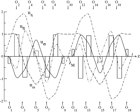
Course of the pseudo fundamental rays u_ω, , u_η and and locations of the octopoles O_ν, ν=1, …, 19, within the ultracorrector.

In order to create such coefficients, the octopole fields must be excited anti-symmetrically with respect to z_M, z_m1 and z_m2, respectively. This anti-symmetric excitation mode of the octopoles does neither produce twofold eikonal coefficients nor coefficients S_κλ^{(4, 2μ)} with κ+λ even.

Correction of the third-order aberrations

The correction of the primary aberrations must start with the elimination of the chromatic aberrations since this procedure also affects the third-order geometrical aberrations. Subsequently, these aberrations are compensated by means of octopoles which do not influence the preceding chromatic correction. The courses of the fundamental rays shown in figure 12 demonstrate that three stigmatic images of the diffraction plane are formed within the corrector. The image located at the plane z_M midway between the two septuplets is undistorted while the image at the center of each septuplet is strongly distorted in first order. Octopoles placed at these planes only affect the axial aberrations because the field rays are zero at these positions. Since the ratio x_α/y_β of the axial rays differs strongly at each octopole location, we can eliminate the third-order axial or aperture aberrations by means of these octopoles. Because they do not introduce off-axial aberrations, it is advantageous to compensate for the axial aberrations in the last step of the correction procedure.

Unfortunately, none of the remaining field aberrations can be eliminated without affecting other aberrations as well. However, we can utilize the fact that a symmetric excitation of the octopoles with respect to the mid-plane z_M produces only eikonal terms with κ+λ even. Hence comas and third-order distortions are not produced for this symmetric excitation mode. These aberrations are formed by the anti-symmetric mode where the octopole field is anti-symmetric with respect to both the mid-plane z_M and the center plane of each septuplet.

In order to eliminate the aberrations largely independently, the octopoles must be placed at optimum positions within the corrector, as shown in figure 13. The best arrangement is achieved by superposing an adjustable octopole field on each quadrupole field of the two septuplets. To enable rotation of the octopole field about the optic axis, twelve-pole elements are necessary. In addition we place twelve-pole elements symmetrically about the central element of each septuplet at positions , where the axial rays x_α and y_β coincide. A further twelve-pole element is centered at the midplane z_M of the corrector. Hence a total of 19 adjustable octopole fields are introduced to compensate for the three complex and the 16 real eikonal coefficients produced by the magnetic round lenses and the quadrupoles of the corrector. The eikonal terms which depend solely on w_o and need not to be eliminated because they do not contribute to the aberrations at the image plane. Employing the symmetric excitation mode of the octopoles, we first compensate for the image curvature and the field astigmatism and subsequently for the axial aberrations. The field astigmatism consists of the conventional round-lens term and a 4-fold term produced by the quadrupole and octopole fields.

To avoid that the correction of an aberration induces aberrations, which have already been corrected, it is necessary to perform the correction in a distinct sequence. In the first step we eliminate the image curvature by means of the octopoles O₂=O₈=O₁₂=O₁₈. Subsequently we compensate for the round-lens field astigmatism by means of the octopoles O₄=O₆=O₁₄=O₁₆. The simultaneous symmetric excitation of four octopoles prevents the formation of 2-fold eikonal terms and of terms with κ+λ odd. In the presence of magnetic lenses the coefficient of the field astigmatism is complex. To compensate for both the real part and the imaginary part, the principle sections of the octopoles must be rotated by a distinct angle with respect to the principal sections of the quadrupole system.

In the third step the 4-fold field astigmatism is corrected by the octopoles O₁=O₉=O₁₁=O₁₉ without affecting the preceding corrections. However, the elimination of this aberration introduces contributions to the axial aberrations, which consist of the spherical aberration and the four-fold axial astigmatism. Its coefficient becomes complex by correcting the anisotropic component of the field astigmatism. As a result the axes of the 4-fold axial astigmatism do not lie anymore on the principal sections of the corrector. The spherical aberration and the 4-fold axial astigmatism are subsequently eliminated by the octopoles O₅=O₁₅ and O₁₀, respectively. The azimuthal orientation of the octopole O₁₀ must be chosen in such a way that the axes of the 4-fold axial astigmatism lie on its principal sections.

Since the central octopoles O₅, O₁₀ and O₁₅ are located at stigmatic images of the diffraction plane, the correction of the axial aberrations does not produce any off-axial aberrations. In order to compensate for the odd terms without affecting the preceding corrections of the even terms, the octopoles must operate in the anti-symmetric mode. The corresponding field is zero at the central octopoles. The remaining 16 octopoles suffice to compensate for eikonal terms with κ+λ odd. Owing to its symmetry, the quadrupole fields of the corrector do not produce such terms. However, the round lens system may introduce two terms with complex coefficients in the presence of magnetic lenses. These coefficients account for the coma and the third-order distortion, respectively. Since these aberrations can be eliminated without the need of a corrector, it is more favorable to compensate for these aberrations by incorporating additional round lenses. In this case only 15 octopoles are required to compensate for all the other third-order aberrations. Hence the octopoles O₃, O₇, O₁₃ and O₁₇ are then obsolete.

Correction of chromatic aberrations

The need for chromatically corrected electron optical systems has recently been revived in the context of in situ high-resolution electron microscopy and high-throughput electron projection lithography [27]. Inelastic scattering due to plasmon excitations within the support film for the mask cause a large energy broadening of several tenths eV. As a result edge resolutions below 80 nm can hardly be realized. In order to achieve resolutions in the order of 20 nm, the additional correction of both the axial chromatic aberration and the chromatic distortion is mandatory. The azimuthal or anisotropic component of the chromatic distortion vanishes if the Larmor rotation between the object and the image plane is zero. This can be achieved by properly adjusting the direction of the current in the coils of the individual round lenses.

The correction of chromatic aberration can readily be performed by substituting crossed electric and magnetic quadrupoles for the quadrupoles located at astigmatic images and/or at the centers of the two septuplets at which strongly distorted images of the diffraction plane are formed. Usually four of these elements are needed to compensate for both the primary axial chromatic aberration and the isotropic or radial chromatic distortion. Chromatic correction is achieved by adjusting the electric and the magnetic strengths of the mixed quadrupoles in such a way that they act partly as first-order Wien-filters whose twofold ‘dispersion’ can be adjusted arbitrarily at least in principle. The corrector depicted in figure 12 is also well suited for simultaneously correcting the chromatic aberrations. Owing to the symmetry of the fundamental rays and of the quadrupole field within each sub-unit shown in figure 11, the corrector is free of first-degree chromatic distortion if an image of the cross-over or the effective source, respectively, is placed at the front nodal plane z_N of the corrector (x_γ(z_N)=y_δ(z_N)=0). The degree is the exponent of the chromatic parameter

which accounts for the energy deviation ΔE=eΔΦ of the electron from the nominal energy eΦ.

Due to the anti-symmetry of the electric and the magnetic quadrupole fields with respect to the mid-plane z_M, the corrector only introduces a rotationally symmetric axial chromatic aberration, but no axial chromatic astigmatism. Considering further the properties of the fundamental rays for the two septuplets, it can be shown that the corrector contributes the term

to the coefficient C_c=C_cR+C_cQ of the axial chromatic aberration of first-degree

at the image plane z_i. The z-integration has to be taken only over the first half of the front septuplet because we have taken into account the symmetry of the quadrupole fields and of the axial rays x_α and y_β, with respect to the mid-planes of the septuplets. The total quadrupole strength G(z) defines the Gaussian optics of the corrector and hence is a fixed function of z. However, the electric quadrupole strength Φ_2c must only fulfill the symmetry requirements with respect to the symmetry planes. Therefore, Φ_2c can be chosen arbitrarily within the first half of the front septuplet. To keep G unchanged it is necessary to adjust the magnetic quadrupole strength Ψ_2s. This condition is met most easily by employing mixed electric and magnetic quadrupoles with identical shape of the electrodes and pole pieces. The excitation of the electric and the magnetic field components is chosen in such a way that each element acts partly as a first-order Wien filter which does not affect electrons with nominal energy.

The relation (70) for the coefficient of the primary axial chromatic aberration demonstrates that the most efficient correction is achieved if crossed electric magnetic quadrupoles are centered at planes where either x_α or y_β are zero, or where these rays largely differ. To prevent that the necessary electric field strengths adopt unrealistic values, the distant axial fundamental ray must be sufficiently large within these correcting elements. This condition can be fulfilled in most cases by properly arranging the quadrupoles within the septuplet. In the simplest case the primary axial chromatic aberration (71) is eliminated by two crossed electric magnetic quadrupoles located at the centers of the two septuplets, without introducing a first-order chromatic distortion. Since astigmatic line images are located within four of the five inner elements of each septuplet, they are also well suited as proper locations for the Wien-filters. Therefore, the total required electric quadrupole strength for correcting the chromatic aberration can be distributed to ten multipole elements of the corrector. In this case the strength of each electric quadrupole field can be kept sufficiently small even at acceleration voltages of about 200 kV.

Owing to the imposed symmetry conditions, the ultracorrector shown in figure 12 does not produce 2-fold first-order chromatic aberrations. As a result all first-order chromatic aberrations are isotropic and rotationally symmetric. Four astigmatic line images of the object and a strongly distorted image of the crossover are formed within each septuplet of this corrector. Considering the symmetry requirements with respect to the midplane of each septuplet, three electric quadrupole strengths can be chosen arbitrarily if first-order Wien filter are placed at each of these images. By properly adjusting the electric quadrupole strengths, it is possible, at least in principle, to compensate for the second-degree chromatic aberration too, thus realizing an electron-optical apochromat. Such a system forms a perfect paraxial image at the same plane for three neighboring wavelengths or energies, respectively [28]. If we correct in addition the spherical aberration by means of the octopole fields, we obtain the exact electron-optical equivalent of a light-optical apochromat. The correction of the second-degree chromatic aberration may be necessary in high-resolution energy filtering electron microscopy to allow for large energy windows. The geometry and the dimension of these systems are ultimately limited by the maximum tolerable electric field strength, which should not exceed about 7 to 8 kV mm⁻¹. If in addition the third-order geometrical aberrations are eliminated, the system is corrected for all aberrations up to the third rank inclusively. The realization of such systems may open new perspectives for nano-science and technology because they represent high-performance electron-optical analogues of sophisticated light-optical systems. The rank of an aberration is defined as the sum of its degree and its Seidel order.

Mirror corrector

The Scherzer theorem states that a particle optical system has a positive spherical aberration when three conditions are satisfied:

• The optics is spherically symmetric.

• The fields are not time dependent.

• The velocity of the reference particle does not change sign.

In an electrostatic mirror, the third condition is not satisfied and the spherical aberration can therefore be corrected. Additionally the chromatic aberration can be corrected. The SMART project aims to build the first microscope that takes advantage of this possibility. Due to the importance of this project for the advancement of the electron microscope, we include results from this project in this section.

Electron mirrors are capable of correcting the primary spherical and chromatic aberration of rotationally symmetric lenses. The resolution of corrected systems is limited by the higher-order axial aberrations which are determined by means of a time-dependent perturbation procedure. This formalism allows one to calculate the geometric aberrations of a rotationally symmetric electromagnetic electron mirror up to arbitrary order. Relativistic effects are taken into account. The symmetry in time with respect to the turning point is utilized to reduce the number of numerical integrations. In addition analytical formulae are given for the coefficients of the spherical and the axial chromatic aberration. The correction properties are illustrated by means of two realistic examples.

The attainable resolution of electron microscopes is limited by the axial chromatic aberration and the spherical aberration. An electron mirror is able to correct these aberrations simultaneously [29]. In this case the remaining higher–rank axial aberrations limit the resolution of the instrument. To investigate the correction properties of mirror correctors and to determine the residual aberrations, a fast calculation procedure is mandatory.

In order to observe the improvement of the resolution by the correction of the primary axial aberrations in practice, we must increase the magnification and the angle of acceptance by the improvement factor. Unfortunately, the required stability of microscopes increases by the square of this factor. Owing to this behaviour, the instabilities and the misalignments may limit the resolution of a corrected microscope.

In the case of low-dose imaging it is advantageous to use the corrector for enhancing the signal-to-noise ratio by increasing the angle of acceptance at the same magnification. This mode of operation requires an improvement of the stability which increases only linearly with the aperture angle. Hence the correction of aberrations is a very promising technique for such applications.

Calculation procedure for electron mirrors

In the conventional theory of aberrations of static fields the coordinate z along the optic axis is considered as the independent variable. This choice is not possible in the case of electron mirrors because the ray gradients diverge near the turning point. Therefore, the position coordinates x=x(t), y=y(t), and z=z(t) of an electron must be described as functions of the independent time variable t [29].

Reference electron

The reference electron is defined as the axial electron which enters the mirror along the optic axis with nominal kinetic energy E_n . The turning point ζ_T of this electron is defined by the relation . The position of an arbitrary electron

is measured with respect to the corresponding position

of the reference electron, as shown in figure 14. Since the electrons are confined to the neighborhood of the optic axis and because the initial velocities of all electrons including the reference electron differ only slightly, the components x, y and h are small quantities. Accordingly, the equation of motion can be expanded with respect to these three coordinates.

Figure 14.

Position (x, y, h) of an electron with respect to the location (0, 0, ζ) of the corresponding reference electron.

Equation of motion

In the case of a mirror it is advantageous to start from the Lorentz equation of motion

where m, −e and are the relativistic mass, charge and position of the electron, respectively. The electric field

is determined by the electric potential ϕ=ϕ(x,y,z) with the gauge

Since the region in the vicinity of the axis is free of charges and currents the magnetic induction

can be written as the gradient of the scalar magnetic potential ψ=ψ(x,y,z).

We denote the axial potentials by

The differential time equivalent is defined by the relation

where

is the relativistically modified potential, c is the velocity of light, Φ_c is the acceleration voltage, and m₀ is the mass at rest of the electron. Since the gauge (76) sets the total energy of the reference electron equal to zero, the total energy of an arbitrary electron

represents its energy deviation δE from the total energy of the reference electron.

In the following calculations dots indicate differentiations with respect to τ and primes denote differentiations with respect to z, ζ, or h. This notation is reasonable since the latter quantities are linearly related with each other (72).

The conservation of energy (83) leads to the formula

for the relativistic mass of an electron with relative energy deviation κ. Using the equations (80) and (84), the path equation (74) adopts the form

Introducing the complex off–axial quantities

the three-dimensional equation (85) decomposes into the two complex equations

It should be mentioned that the relative energy deviation κ is not a free parameter, since the energy of an electron is fixed by its initial position and velocity .

For the reference electron (κ=0, w=0, z=ζ) the equation (88) simplifies considerably. Multiplying the resulting equation with and integrating with respect to τ we find the conservation of energy in the simple form

Within the potential Φ=Φ_c of the column the normalized velocity of the reference electron is . In this case differentiations with respect to τ and z are identical apart from the sign. This behaviour is a consequence of our special choice (80) of the time parameter τ.

In the presence of a magnetic field it is advantageous to choose the rotating u, z coordinate system, where the complex off-axial coordinate u is given by

The angle

accounts for the Larmor rotation. Replacing z by the relation (72), the equations (87) and (88) are transformed into equations for u and h.

Employing the complex notation, the electric field is connected with the electric potential via the relations

The electric potential is derived from the Laplace equation

with the assumption that the axial potential Φ(z)=Φ(ζ+h) is known. Starting from (95), we expand the electric potential in a power series with respect to the coordinates u, and h:

where Φ^[n] denotes the nth derivative of Φ with respect to z and

The equivalent expansion of the scalar magnetic potential leads to the expression

Expanding each of the equations of motion (92) and (93) in a power series with respect to the coordinates u, , and h and using the abbreviations

we may write these equations as

The functions Λ and θ vanish in the non-relativistic limit ε=0. The perturbations

contain all nonlinear terms in the coordinates u, and h.

Since the electric and the magnetic axial potential have the symmetry

with respect to the time parameter τ, symmetric and antisymmetric solutions exist for the differential equations (101) and (102).

Linear approximation

The linear approximation of the equations (101) and (102) leads to the relations

The lateral equation (107) formally coincides with the well-known paraxial path equation of rotationally symmetric systems. The solution of this equation yields the Gaussian approximation of the trajectories. The solution of the axial equation (108) shifts the image plane and only affects the aberrations. The part of the solution, which results from the inhomogeneity of equation (108), accounts for the relativistic modification of the axial chromatic aberration.

Lateral fundamental rays

The lateral equation (107) has two linearly independent solutions. To obtain a symmetric and an antisymmetric trajectory u_μ and u_ξ, we must impose the initial conditions

on these solutions. With this choice the Wronskian is

An arbitrary paraxial ray can be written as the linear combination

of the real fundamental rays u_μ and u_ξ; the coefficients μ and ξ may be complex. In most cases analytical solutions of (107) do not exist and the fundamental rays must be calculated numerically. The coefficients are determined by the asymptote of the incident electron ray.

Axial fundamental deviations

The function

is the antisymmetric solution of the homogeneous part of equation (108); the symbol

accounts for the change of the sign at τ=τ_T.

Using the Wronskian

and the relation (112), we can express the solution h_σ as

The lower integration limit τ_σ must be chosen in such a way that h_σ gets symmetric, i.e. .

By a partial integration of (115) we get the alternative representation

which does not require the knowledge of τ_σ. However, since both representations (115) and (116) contain diverging integrands, the direct numerical solution of the differential equation (108) may be a better alternative.

Due to the conditions

the axial fundamental deviations fulfill the relations

in the field-free region of the column. These properties are a consequence of the conservation of energy.

Employing the method of the variation of constants, we obtain the special solution h_κ of the inhomogeneous differential equation (108) as

The course of this deviation is symmetric with respect to τ_T. The linear approximation of the axial deviation results in

where σ and ν are real coefficients which will be specified in the next sections. It should be noted that the inhomogeneous part κ h_κ vanishes in the non–relativistic limit.

Examples

The time-dependent formalism does not offer the possibility to eliminate high derivatives of the electric and magnetic axial potentials by partial integrations. For example the expression for the coefficient of the third-order spherical aberration contains Φ^[4]. The evaluation of the fifth-order spherical aberration even requires Φ^[6].

The charge simulation method is the most appropriate way to precisely determine such high derivatives of the electric field since it allows the analytical differentiation of the corresponding potential distributions. We have used a simple model which places ring charges inside the electrodes close to the surfaces.

Diode mirror

To illustrate the imaging properties of an electron mirror, we have studied a purely electric mirror consisting of two electrodes. Figure 15 shows the arrangement and the shape of the electrodes and several equipotentials. The resulting path of the reference electron ζ and that of the fundamental rays u_μ, u_ξ and the axial deviations h_σ and h_ν with respect to τ are depicted in figure 16. The course of the fundamental rays along the optic ζ-axis is shown in figure 17.

Figure 15.

Sectional view and equipotentials of a diode mirror with bore radius r in the case Φ_m=-0.25 Φ_c. The circular edges of the electrode surfaces have a radius of 0.4 r. The equipotentials are labeled in units of the column potential Φ_c.

Figure 16.

Paths of the reference electron ζ, of the fundamental rays u_μ, u_ξ and of the axial deviations h_σ and h_ν as functions of τ. The optic axis intersects the surface of the mirror electrode at the origin of the coordinate system.

Figure 17.

Paths of the fundamental rays u_μ, u_ξ and of the axial deviations h_σ and h_ν as functions of ζ. The slope of u_ξ and h_ν diverges at the turning point ζ_T=0.865431 r. The ray u_μ intersects the optic axis at ζ_m=7.73760 r.

To survey the properties of this mirror, we assume non–relativistic conditions and put the potential of the mirror electrode at Φ_m=−0.25 Φ_c. The final slope of the axial ray is chosen as . The origin of the z-coordinate was placed at the surface of the mirror electrode. In this case the turning point is located at ζ_T=0.865431 r, where r is the radius of the column electrode.

We used a step-controlled Runge–Kutta method of fourth order and a trapezoidal integration to obtain the characteristic elements of the mirror. The results show that the fundamental ray u_μ intersects the optic axis asymptotically at ζ_m=7.73760 r. The coefficients of the axial chromatic and of the spherical aberration are R_ωκ=0.187461 r and , respectively. The coefficients of the axial aberrations of higher rank are found as , and R_ωκκ=−0.0777 r. All values are accurate up to the last digit inclusively. The accuracy was checked by observing the convergence with increasing number of ring charges and Runge–Kutta steps. The maximum number of charges was 2000 and the maximum number of steps was 4000.

Tetrode mirror

In the previous example all imaging properties are determined by the potential Φ_m of the mirror electrode. In order to properly adjust the correcting properties, we must introduce additional free parameters. By increasing the number of electrodes which are put at arbitrary potential, we provide the proper variability. Figure 18 shows an arrangement that consists of four electrodes. Since the potentials Φ_m, Φ₁ and Φ₂ affect the distribution of the axial potential in different regions, it is possible to properly adjust the focal length, the chromatic aberration and the spherical aberration.

Figure 18.

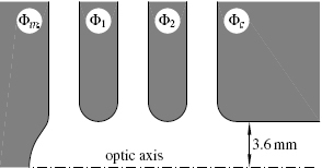
Sectional view of a tetrode mirror. The potentials Φ_m, Φ₁ and Φ₂ determine the focal length, the chromatic aberration and the spherical aberration.

We investigated the properties of this tetrode mirror whose Gaussian object and image plane have been placed at the same fixed position of about 210 mm in front of the mirror electrode. The result shown in figure 19 demonstrates that the axial chromatic and the spherical aberration can be adjusted within a wide range. This region is sufficiently large to enable the correction of the corresponding aberrations of a rotationally symmetric objective lens for various modes of operation.

Figure 19.

Variation range of the tetrode mirror shown in figure 18. The coefficient of the chromatic aberration R_ωκ and that of the spherical aberration can be adjusted within the shaded area, while the Gaussian image plane remains fixed at a distance of 210 mm from the mirror electrode.

The feasible incorporation of an electron mirror into an electron microscope necessitates a beam separator. Rempfer [30] utilized a dispersive system of homogeneous deflection magnets and showed experimentally the correction capability of mirrors. However, for significantly increasing the resolution and/or the angle of acceptance, a dispersion-free beam separator is necessary. We proposed in [31] a possible arrangement using the sharp cut-off fringing field approximation. The realization of such a device necessitates the exact evaluation of the magnetic field.

The corrected system depicted schematically in figure 20 will be implemented into a photo-emission spectro–microscope which is presently under construction [32]. The calculations showed that on the premises of a precise adjustment the corrector should improve the resolution up to a factor of ten. The corresponding increase of the angle of acceptance enables one to utilize 100 times more scattered or emitted electrons than without correction. This improvement is very important for the photo–emission mode.

Figure 20.

Scheme of a corrected system. The tetrode mirror is implemented via a dispersion-free magnetic beam separator. The thin shaded regions indicate the induction coils, which are placed at the surface of the pole plates (© 2002 Springer [34]).

Figure 21.

Horizontal xz cross-section through the omega-shaped electrostatic monochromator and course of the fundamental rays along the straightened optic axis within the horizontal and the vertical sections.

Monochromator

The ultimate goal of high-resolution analytical electron microscopy is the acquisition of detailed information about the atomic structure, the chemical composition and the local electronic states of real objects whose structure deviates from ideal crystalline periodicity. To obtain detailed information on the interatomic bonding an energy resolution of about 0.2 eV is necessary. Unfortunately, the presently available electron microscopes cannot fulfill this requirement because electron sources with a maximum energy spread of 0.2 eV at a sufficiently high current do not yet exist for conventional transmission electron microscopes. To realize such a source, we have designed an electrostatic monochromator, which reduces the energy spread of the illuminating beam [10]. The monochromator is placed behind the gun and removes all electrons whose energies deviate more than ±0.1 eV from the most probable energy. In the case of a Schottky field emitter, the monochromator takes away about 70% of the emitted electrons. In order to preserve the emission characteristic of the source and to prevent a loss of lateral coherence, the dispersion must vanish on the far side of the monochromator, as illustrated schematically in figure 22.

Figure 22.

View of the toroidal deflection elements and the dispersive properties of the electrostatic monochromator.

Energy filtering is performed within the monochromator at a line-shaped image of the source where the dispersion is at its maximum. The omega-shaped monochromator shown in figure 21 consists of four electrostatic deflectors which are symmetrically arranged about the symmetry plane. Recently, this monochromator has been incorporated together with the MANDOLINE filter [33] into the SESAME Microscope at the Max-Planck Institute in Stuttgart. This high-performance analytical electron microscope enables local electron spectroscopy with an energy resolution of about 0.1 eV, which is necessary for determining local variations of the atomic bonding near interfaces or defects.

Imaging energy-filters

In order to fully exploit the capability of the monochromator, it must be combined with a high-performance imaging energy filter. Such a filter must possess (a) a large dispersion to allow for sufficiently small energy windows, (b) no second-order aberrations at the image and the energy selection plane, and (c) a compact geometry to avoid an unduly large lengthening of the microscope column. The latter requirement is especially important in the case of aberration-corrected analytical electron microscopes, because the incorporation of the monochromator and the energy filter further lengthen the column in addition to the corrector. As a result, the mechanical instabilities increase and may impede an appreciable reduction of the information limit below 1Å. Due to intense efforts by several manufacturers, the mechanical and electrical stabilities of atomic-resolution electron microscopes have improved recently to such an extent that an information limit of about 0.5 Å has been reached. However, the incorporation of the aberration corrector and the imaging energy filter may rise this limit. Therefore, one must further improve the information limit in order to achieve a point resolution of 0.5 Å which is the goal of the US TEAM project.

MANDOLINE-filter

The required properties of a high-performance imaging energy filter are best met by the MANDOLINE filter which has by far the highest dispersion and transmissivity of all energy filters proposed so far. This filter is free of second-order aberrations and has a very high dispersion.

The MANDOLINE filter shown in figure 23 consists of a single homogeneous bending magnet and two inhomogeneous deflection magnets with tapered pole pieces. These elements focus the electrons within their two principle sections towards the optic axis and act as ‘anamorphotic’ lenses with a curved axis. They allow large deflection angles yielding a high dispersion. This behavior differs from that of homogeneous magnets where the vertical refraction is confined to the short fringing-field regions at the entrance and exit faces of the magnet. The geometry of the tapered pole pieces of an inhomogeneous sector magnet is shown schematically in figure 24. Although the MANDOLINE filter enlarges the column only by about 23 cm, its dispersion is about twice as high as that of the best post-column filter. Half of the second-order aberrations are eliminated by the symmetric arrangement of the magnets and the symmetry of the fundamental rays with respect to the midplane of the filter. The remaining aberrations are compensated for by six sextupoles placed in the drift space between the homogeneous magnet and the conical magnets. To preserve the required mid-plane symmetry, the sextupoles are exited in pairs.

Figure 23.

Schematic arrangement of the deflection elements and the sextupoles within the MANDOLINE filter, the distance between the energy selection plane and the diffraction image in front of the filter defines the lengthening of the column.

Figure 24.

Geometry of a conical bending magnet producing homogeneous dipole and quadrupole fields along the circular axis in the region between the tapered poles (© 2002 Springer [34]).

W-filter

Each additional element incorporated into the microscope enlarges the length of the column increasing its mechanical sensitivity. We can significantly suppress the mechanical instabilities by placing the heavy energy filter at the bottom of the instrument. To achieve a compact and stable microscope, it is advantageous to design it as a twin-column instrument such that the second column contains the projector lenses and the detection system. Since the optic axis in the ‘image’ column is parallel to that of the ‘object’ column, the filter must also reverse the direction of flight of the electrons. Hence, the total deflection of the filter must amount to 180°, in contrast to the straight-vision in-column filters proposed so far [34]. In accordance with the conventional nomenclature, we denote our beam-reversing filter as ‘W-filter’, owing to the pronounced W-shaped course of its optic axis. The filter can be considered as an Ω-filter placed between two bending magnets with equal deflection of the optic axis. For a total deflection of 180°, the entrance axis and the exit axis are parallel to each other. In this case mechanical momenta are avoided because the object and image columns rest perpendicular on the filter, which acts as their common base. The two columns can be further stiffened by proper mechanical connections. The resulting twin column will be significantly shorter and less sensitive with respect to mechanical instabilities than the conventional single-column electron microscopes.

The separation s of the two column axes depends on the radius of curvature R_ν and on the angular deflection φ_ν of the optic axis within the constituent bending magnets ν=1, 2, …, N of the filter.

Within the frame of validity of the SCOFF approximation such an element produces a constant magnetic quadrupole strength Ψ_2s along the optic axis. In order that the filter does not introduce second-order distortions at the final image plane, pairs of identical deflection elements are arranged symmetrically about the midplane z_m of the filter, as shown in figure 25. Owing to this symmetrical arrangement, the filter is also free of second-order axial aberrations. In order to avoid large higher-order aberrations the fundamental paraxial rays must remain close to the optic axis within the entire filter. This condition is best achieved for a telescopic filter, where the fundamental axial rays x_α and y_β run parallel to the optic axis in front of and behind the filter.

Figure 25.

Arrangement of the bending magnets and the sextupoles for the corrected 90° W-filter operating in the type I mode (© 2002 Springer [34]).

Gaussian optics

For determining the paraxial properties of the energy filter we introduce the curved xyz-coordinate system. The curved z-axis and the horizontal x-axis are embedded in the midsection of the magnets, while the vertical y-axis is perpendicular to it. The curvature of the optic z-axis

is determined by the dipole strength Ψ_1s of the magnets taken along the axis. The course of the paraxial trajectories within the region of the magnets is governed by the Gaussian path equations [35, 36]

The inhomogeneous term on the right-hand side of the equation (123) considers the dispersive effect of the energy deviation ΔE of the electron from the nominal energy E₀. This perturbation is proportional to the relativistically modified relative energy deviation

Equation (123) becomes homogeneous for monochromatic electrons with nominal energy (ΔE=0). We define the fundamental rays at the image z_D of the diffraction plane located in front of the filter. The fundamental rays x_α, x_γ, y_β and y_δ are linearly independent solutions of the paraxial path equations (123) and (124). In the case of telescopic filters, the axial rays x_α and y_β run parallel to the optic axis in front of and behind the filter. These rays start with unit slope from the center of the object plane z_o. Therefore, they have the off-axial distance f_oM_D in front of the filter, where f_o and M_D are the focal length of the objective lens and the magnification (M_D≪1) of the diffraction plane, respectively. We fix the axial rays by imposing the conditions

As a result, the rays start from the center of the object plane with slope 1/M_D. The two field rays x_γ and y_δ pass through the centers of the planes z_d and z_D. We fix these rays by imposing the conditions

Owing to these boundary values, all fundamental rays have the dimension of a length. As a consequence, the constants of the Helmholtz–Lagrange relations coincide with the focal length of the objective lens:

Employing these fundamental rays, the components of the paraxial ray are given by the simple linear combinations

The angles α, β, γ and δ are connected with the initial parameters α_o, β_o, x_o, y_o of the ray at the object plane z_o via the relations

The dispersion ray x_κ is the inhomogeneous solution of the equation (123) for the special case κ^∗=1. Owing to the boundary conditions (127) for the field rays, the relation

holds at the final image plane z_i; M_i defines the magnification of the object at this plane. Note that the intermediate images of the diffraction plane are demagnified if those of the object are magnified.

Examples

In the case of straight-vision systems, the deflection angles φ_ν of all bending magnets add up to 0° for the ‘omega’ filter and to 360° for the ‘alpha’ and ‘gamma’ filters [28]. Standard post-column filters have a deflection angle of 90°, while the total deflection angle of the W-filter amounts to 180° because the optic axis reverses its direction. To obtain a high dispersion, the curvature Γ of the optic axis changes its sign twice within the W-filter. We achieve the alternating curvature and a high dispersion by means of two pairs of conical sector magnets with large deflection angles φ_ν and opposite excitations. For simplicity, we presuppose that all N magnets have the same radius of curvature

Within the frame of validity of the SCOFF approximation this radius is constant inside the box-shaped field of each magnet and zero outside. The quadrupole strength of the conical magnets,

depends on the inclination angle δ of the inner pole faces, the vertical distance D between these poles taken at the optic axis and on the absolute value of the dipole strength Ψ_1s. We employ sextupole elements to compensate for the non-vanishing second-order aberrations. These elements must be arranged in pairs symmetrically about the midplane z_m of the system in order to avoid distortion and axial aberrations. The symmetric arrangement of all elements guarantees that these aberrations are absent for the system as a whole. To compensate simultaneously for the axial aberration at the energy selection plane and for the aberrations (inclination of image field and field astigmatism) at the final image plane, a strongly astigmatic path of the paraxial rays within the regions between the bending magnets is mandatory [35]. We eliminate the aberrations largely independently from each other by placing the sextupole elements at astigmatic images of the object plane and the diffraction plane, respectively [35, 37]. For this purpose it is advantageous to insert three pairs of sextupole magnets, as shown in figure 23 and 25. The single sextupole centered at the midplane z_m of the MANDOLINE and the W-filter automatically fulfills the symmetry condition. To minimize the non-vanishing aberrations of the W-filter, the first and third bending magnet are made equal. They are placed in opposite x-direction to reverse the deflection. Owing to the required midplane symmetry, the first magnet coincides with the sixth magnet and the third magnet with the fourth magnet. Since the deflection angles of these bending magnets cancel out, the second and the fifth magnet must each deflect the axis by 90° in order to achieve a total deflection of 180°. The energy selection plane z_E is conjugate to the diffraction plane z_D located in front of the filter. By considering the relations x_γ(z_E)=0 and x_α(z_E)=f_o, we obtain for the lateral displacement of the dispersion ray at the energy selection plane the expression

where C_γκ is the dispersion coefficient. In order to achieve a large dispersion, we must adjust Ψ_1s and x_γ in such a way that the product Ψ_1sx_γ does not change its sign inside the filter. Hence if two adjacent bending magnets deflect the electrons in opposite directions, the field ray x_γ must intersect the optic axis in the field-free region between these magnets. The dispersion (displacement per eV)

is proportional to the dispersion coefficient and influenced by relativistic effects for nominal energies E₀ larger than about 100 keV.

We impose that astigmatic images of both the object plane and the diffraction plane are located at the midplane z_m of the filter. This is only possible if the two line images are perpendicular to each other. In this case, the fundamental field rays must satisfy the conditions

Because the fundamental rays are entirely defined by the initial constraints (126) and (127), we can only meet the additional conditions (136) by adjusting four free parameters of the system appropriately. The adjustable parameters are the quadrupole strengths of the conical bending magnets and the spacing between these elements. The normalized quadrupole strength defines the so-called field index of the inhomogeneous magnet:

This index is zero for homogeneous bending magnets with plane-parallel inner pole faces. We have two adjustable field parameters ν₁=ν₃ and ν₂. The two other free parameters are the spacing a between the magnets of each half of the filter and the separation distance 2g between these halves. Therefore, the proposed doubly symmetric system provides exactly the number of free parameters which are necessary to adjust the required path of the paraxial fundamental rays. For the special system shown in figure 25 the distances a and g coincide, as well as the quadrupole strengths (ν₁=ν₂). Although the rays x_α and x_γ do not possess any symmetry with respect to the central planes z_s1 and z_s2 of each half of the filter, these rays are connected by a peculiar symmetry property. Within each half of the filter the course of the axial ray x_α is mirror-symmetric with respect to that of the field ray x_γ apart from a constant factor b:

In order to achieve a high dispersion, x_γ must neither be antisymmetric with respect to z_s1 and z_s2, respectively, nor symmetric. However, the fundamental rays y_β and y_δ can be symmetric or antisymmetric with respect to these planes because these rays do not affect the dispersion. Since they are linearly independent from each other, one ray must be symmetric and the other one antisymmetric. Depending on the chosen symmetry for y_β and y_δ, two types of doubly symmetric W-filters exist. We name the filter to be of type I if the course of the ray y_δ is symmetric with respect to z_si and of type II if it is antisymmetric.

The schematic arrangement of the magnets for the filter of type I is shown in figure 25 together with the sextupoles for correcting the second-order aberrations. The course of the fundamental rays along the straightened optic axis within the first half of this filter is depicted in figure 26.

Figure 26.

Course of the fundamental paraxial rays along the straightened axis of the first half of the W-filter depicted in figure 25 (© 2002 Springer [34]).

Owing to the relatively small spacing between the magnets, the positions of the sextupoles are largely fixed, apart from the two sextupoles, which are placed in front of and behind the filter, respectively. The dispersion ray x_κ shown in figure 27 starts with zero slope in the first magnet and oscillates with increasing amplitude along the optic axis inside the filter. The ray adopts its maximum off-axial distance at the exit of the last magnet. Since x_κ leaves this magnet parallel to the optic axis, the dispersion at the energy selection plane does not depend on its distance g=a/2 from the filter. The comparison of the dispersion coefficients for the two filter types reveals that the type II filter produces a significantly larger dispersion than the type I filter. Accordingly, filters of type II should be preferred in practice. Moreover, the large spacings between the magnets of this filter allow one to position more than one sextupole into each of these regions.

Figure 27.

Oscillating path of the dispersion ray x_κ along the straightened optic axis of the W-filter shown in figure 25 (© 2002 Springer [34]).

In order to further enlarge the dispersion without increasing the distance s between the entrance axis and the exit axis, the deflection angles φ₁=φ₃ of the first and third magnet must be larger than 90°. However, the increase in these angles cannot be made substantially larger than about 25°, because the magnets must neither overlap with each other nor with the round lenses of the microscope. The filter depicted in figure 28 satisfies these design criteria. The SCOFF parameters of this system are:

The comparison of the dispersion coefficient C_γκ with those for the systems (139) and (140) reveals that the filter (141) yields by far the highest dispersion for a given distance s between the axes of the two columns. The course of the paraxial rays along the straightened optic axis is shown in figure 29 for one half of the filter. In the vertical yz-section the axial ray y_β is symmetric and the field ray y_δ antisymmetric with respect to the central plane z_s1. Since such a symmetry does not exist for the corresponding rays x_α and x_γ in the horizontal xz-section, the paraxial path of the rays is largely astigmatic within the entire region of the filter.

Figure 28.

Arrangement of the conical bending magnets for the highly dispersive 115° W-filter operating in the type II mode (© 2002 Springer [34]).

Figure 29.

Course of the fundamental paraxial rays along the straightened optic axis of the type II W-filter shown in figure 14 (© 2002 Springer [34]).

This behavior enables one to compensate for the nonvanishing second-rank aberrations by means of sextupoles. These correction elements should be placed at appropriate positions between the bending magnets, in order to eliminate the different aberrations largely independently from each other. Contrary to the geometrical fundamental rays, the dispersion ray x_κ does not possess any symmetry properties, as can be seen from figure 30.

Figure 30.

Path of the dispersion ray x_κ within the 115° W-filter (© 2002 Springer [34]).

The quadrupole strengths ν₁ and ν₂ of the 115° W-filter differ only slightly from each other. For practical reasons it would be very desirable to employ a system whose magnets have the same quadrupole strength. Therefore, the question arises if such a system with a deflection angle close to 115° does exist. The calculations have shown that this is indeed the case, for a deflection angle φ₁=φ₃=121.87°. The parameters of the corresponding filter are

The courses of the fundamental paraxial rays and that of the dispersion ray within this filter hardly differ from those of the 115° W-filter. The dispersion coefficient (143) of the filter roughly coincides with the distance s between the axes of the two constituent columns of the microscope.

Unfortunately, the two symmetric branches of the optic axis come very close to each other within the region of the central bending magnets, as demonstrated in figure 31. Since the pole faces of the adjacent magnets are inclined in opposite directions, the quadrupole field of each magnet will be affected by the adjacent magnet. If this effect prevents a precise alignment of the filter, one can alternatively substitute a homogeneous magnet for the two central conical 90° deflection magnets. The resulting system represents a generalized MANDOLINE filter. The parameters of these filters must be determined by the calculation procedures that have been employed for the MANDOLINE filter [33].

Figure 31.

Arrangement of the doubly symmetric W-filter in the case that the inclination angles of the tapered pole pieces coincide for all magnets (© 2002 Springer [34]).

Second-rank aberrations

The primary aberrations of imaging energy filters are of second rank in the ray-defining parameters α, β, γ, δ and κ∗. According to the nature of these parameters the aberrations can be subdivided into two classes, one comprising the second-order geometric aberrations and the other one the second-rank chromatic aberrations. The order of an aberration is defined as the sum of the exponents of the geometric ray parameters, while the exponents of the ray parameter κ∗ describes the degree of the aberration. The sum of the order and the degree is called the rank. It is an appropriate measure for the magnitude of an aberration [37]. The aberrations represent the deviation of the electron trajectory from its paraxial approximation at the observation plane. In an energy-filtering electron microscope this plane is either the final image plane z_i or the energy selection plane z_E where the energy-loss spectrum is formed. The second-rank aberrations are obtained most conveniently from the third-rank term of the perturbation eikonal taken at these planes. This third-rank eikonal consists of a geometric term and a chromatic term, which has not been considered in the perturbation formalism outlined in section 3. The geometric term is entirely produced by the dipole and hexapole fields of the energy filter, while the chromatic term also contains contributions from the round lenses and quadrupoles of the entire electron optical system. Here we consider only the contribution of the energy filter to the second-rank aberrations. In this case the corresponding third-rank eikonal E_F⁽³⁾ of the filter is constant in the region behind the filter, in particular

To simplify the expressions for the aberrations, we introduce the modified eikonal

which has the dimension of a length. It represents the third-order deviation of the optical path length from its paraxial approximation. The eikonal term is composed of at most 18 monomials in the expansion parameters. Ten of these monomials are entirely of geometric nature. In systems with midplane symmetry five of these monomials vanish and adopts the reduced form

At the observation planes z_i and z_E two of the four paraxial fundamental rays vanish. As a result, the second-rank aberrations at these planes are related with the third-rank eikonal via the expressions

For symmetric filters we have

because such filters image the plane z_D, located in front of the filter, with unit magnification M_E=1 into the energy selection plane z_E behind the filter. If we refer the image aberrations back to the object plane, the relations (147) must be divided by the total magnification

yielding

The axial chromatic aberration of the filter is determined by the coefficients C_αακ and C_ββκ of the eikonal term (146). Since these coefficients are proportional to the square of the ratio f_o/R≪1, the corresponding monomials in the expression (146) are negligibly small. For symmetric filters the coefficients of the chromatic aberration of magnification are related to those of the field aberrations by the relations

The chromatic aberrations with coefficients C_δδκ, C_ακκ and C_γκκ are negligibly small at the final image plane and of no concern for the resolution of the energy loss spectrum located at the plane z_E [36]. The remaining coefficients have been calculated for the doubly symmetric 115° W-filter by employing the SCOFF approximation. The resulting values

demonstrate that the coefficients A_γγγ and B_γδδ of the aperture aberration at the energy selection plane and the coefficient C_γγκ of the axial chromatic aberration at this plane are much larger than those of the field aberrations, because the focal length f_o of the objective lens is very small compared with the radius of curvature R of the bending magnets. Although the coefficient A_ααγ is small, the coefficient

of the chromatic aberration of magnification is rather large. Therefore, it is necessary to eliminate this aberration, together with the axial aberrations at the energy selection plane by external sextupoles. These elements must be centered in pairs symmetrically about the midplane of the filter along the optic axis. In order to correct the individual aberrations largely independently from each other, it is advantageous to place the sextupoles at or near astigmatic images of both the object plane and the diffraction plane. The location of these images are given by the zeros of the paraxial fundamental rays x_α, y_β, x_γ and y_δ.

Conclusion

In the last decade considerable theoretical and experimental progress has been made in the field of electron optics. Thanks to the development of efficient procedures for calculating and designing complex electron-optical systems, it has become possible to precisely design multi-element aberration correctors, imaging energy filters, monochromators and quadrupole systems operating as projector lenses with very small focal length. The incorporation of these elements in the TEM will enable quantitative analytical electron microscopy with sub-Å spatial resolution and energy resolution below 0.1 eV. Moreover, fast computer-added alignment procedures have been established which show the state of alignment and determine the voltages and currents which are subsequently applied by microprocessors to the stigmators compensating for the residual aberrations. Recently, the electrical and mechanical stabilities of the electron microscopes have been improved to such an extent that the information limit has been pushed down to about 0.5Å. So far, the hexapole corrector in combination with a monochromator has achieved resolution limits below n order to further improve the resolution at voltages below 300 kV, the correction of the chromatic aberration is mandatory. Unfortunately, the hexapole corrector cannot compensate for this paraxial aberration because the hexapole fields do not affect the Gaussian rays. The TEAM project aims for a resolution limit of 0.5 Å which equals the radius of the hydrogen atom. In addition, all points of an extended object field must be imaged with the same resolution. To achieve this very demanding goal, we have designed an ultracorrector [26], which provides in combination with the objective lens an achromatic electron-optical aplanat free of chromatic aberration, spherical aberration and isotropic and anisotropic coma. In order to reduce the number of elements, we have utilized for the design of the TEAM corrector the symmetry properties of the hexapole corrector. A telescopic quadrupole quintuplet is substituted for each hexapole. The chromatic aberration is compensated by means of the central electric and magnetic quadrupole of each quintuplet. This element focuses the rays and acts simultaneously as a Wien filter compensating for the chromatic aberration in one of the two principal sections. The spherical aberration and the off-axial coma are eliminated by means of octopoles. The incorporation of each additional element into the electron microscope enlarges the length of the column, increasing the mechanical instabilities. However, in order to achieve high mechanical stability, the instrument must be kept short and compact. We can circumvent these contradicting requirements by splitting the column up in two parts, as shown in figure 32. The imaging energy filter is of the W-type and serves as the common solid base for the two columns which we denote as the object column and the image column, respectively. The filtered achromatic intermediate image plane behind the filter is imaged by means of two quadrupole triplets onto the detector. This quadrupole projector system enables a variable magnification over a very large range [38]. The successful correction of the spherical aberration by Haider et al [8] has been the decisive step for initiating intensive efforts to improve the performance of the electron microscope. Aberration correction combined with monochromator and imaging energy filter will change the microscope from an instrument providing pictures to an analytical instrument giving quantitative information on the atomic structure, elemental composition and the electronic structure of the object with an energy resolution below 0.1 eV. We can expect that future electron-optical instruments will reach a degree of perfection comparable to that attained in light optics.

Figure 32.

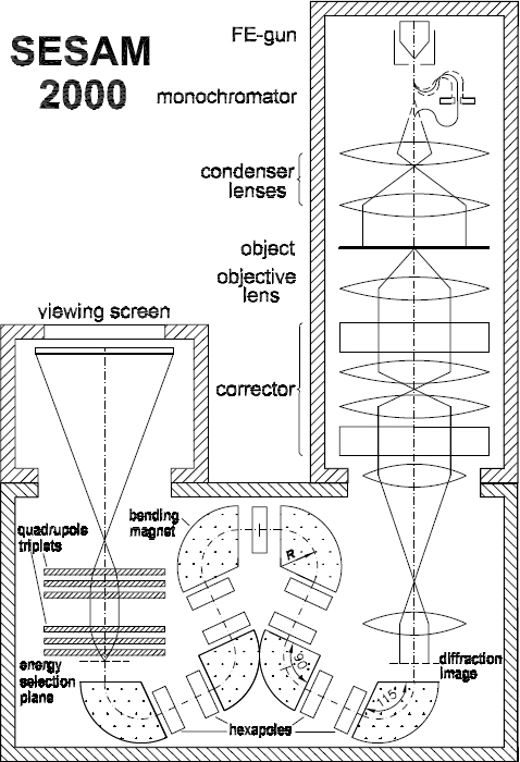
Scheme of the SESAM 2000 illustrating the arrangement of the constituent elements.

References

- deBroglie L D. Ann. Phys. Fr. 1925;3:22. [Google Scholar]
- Busch H. Ann. Phys. Lpz. 1926;81:974. doi: 10.1002/andp.19263862507. [DOI] [Google Scholar]
- Ruska E. and Knoll M. Z. Tech. Phys. 1931;12:389. [Google Scholar]
- Crew A V, Wall J. and Walter L M. J. Appl. Phys. 1968;30:5861. doi: 10.1063/1.1656079. [DOI] [Google Scholar]
- Castaing R. and Henry L. J. Microscopie. 1964;3:133. [Google Scholar]
- Lanio S, Rose H. and Krahl D. Optik. 1986;73:56. [Google Scholar]
- Scherzer O. Z. Phys. 1936;101:593. doi: 10.1007/BF01349606. [DOI] [Google Scholar]
- Haider M, Rose H, Uhlemann S, Kabius B. and Urban K. J. Electron. Microsc. 1998;47:395. doi: 10.1093/jmicro/dfp021. [DOI] [PubMed] [Google Scholar]
- Krivanek O L, Dellby N. and Lupini A R. Ultramicroscopy. 1999;78:1. doi: 10.1016/S0304-3991(99)00013-3. [DOI] [Google Scholar]
- Kahl F. Darmstadt: University of Technology; 1999. Dissertation. [Google Scholar]
- Rose H. Ultramicroscopy. 1999;78:13. doi: 10.1016/S0304-3991(99)00025-X. [DOI] [Google Scholar]
- Rose H. Ultramicroscopy. 2005;103:1. doi: 10.1016/j.ultramic.2004.11.017. [DOI] [PubMed] [Google Scholar]
- Zach J and Haider M. 1995. Nucl. Instrum. Methods. Phys. Res.A 363 316 10.1016/0168-9002(95)00056-9 [DOI] [Google Scholar]
- Hartel P, Preikszas D, Spehr R, Müller H. and Rose H. Adv. Imag. Electron Phys. 2002;120:41. [Google Scholar]
- Rose H. Nucl. Instrum. Methods Phys. Res. 1987;A258:374. [Google Scholar]
- Hoffstätter G H.1995Proc. PAC94, Dallas/TX [Google Scholar]
- Wüstefeld G. DESY: Hamburg/Germany; 1999. Proc. Workshop, ‘Polarized Protons at High Energies’. [Google Scholar]
- Luccio A and Roser T. 1994Third Workshop on Siberian Snakes and Spin Rotators(BNL-52453, Brookhaven National Laboratory Upton/NY) [Google Scholar]
- Goldstein H. Reading MA: Addison-Wesley; 1980. Classical Mechanics. [Google Scholar]
- Born M. and Wolf E. Oxford: Pergamon Press; 1975. Principles of Optics. [Google Scholar]
- Beck V. Optik. 1979;53:241. [Google Scholar]
- Rose H. Nucl. Instrum. Methods. 1981;187:187–99. doi: 10.1016/0029-554X(81)90488-2. [DOI] [Google Scholar]
- Hawkes P W. and Kasper E. London: Academic; 1996. Principles of Electron Optics, vol. 1: Basic Geometrical Optics. [Google Scholar]
- Scherzer O. 1970. unpublished [Google Scholar]
- Rose H. Optik. 1971;34:285. [Google Scholar]
- Rose H. 2004. Nucl. Instrum. Methods Phys. Res.A 519 12 10.1016/j.nima.2003.11.115 [DOI] [Google Scholar]
- Kabius B, Haider M, Uhlemann S, Schwan E, Urban K. and Rose H. Annu. Proc. Micros. Microanal. 2001;59:902. [Google Scholar]
- Rose H. Optik. 1970;32:144. [Google Scholar]
- Rose H and Preikszas D. 1995. Nucl. Instrum. Methods A 363 301 10.1016/0168-9002(95)00065-8 [DOI] [Google Scholar]
- Rempfer G F. and Mauck M S. Optik. 1992;92:3. [Google Scholar]
- Rose H. and Preikszas D. Optik. 1992;92:31. [Google Scholar]
- Fink R. et al J. Electron. Spectrosc. Relaf. Phenom. 1997;84:231. doi: 10.1016/S0368-2048(97)00016-9. [DOI] [Google Scholar]
- Uhlemann S. and Rose H. Optik. 1994;96:163. [Google Scholar]
- Rose H. Advances in electron optrcs High-Resolution Imaging and Spectrometry of Materials (Springer Series in Materials Sources) In: Ernst F, Rühle M, editors. vol 50. Heidelberg: Springer; 2002. p. pp 189–270. [Google Scholar]
- Rose H. Optik. 1978;51:15. [Google Scholar]
- Lanio S. Optik. 1986;73:99. [Google Scholar]
- Rose H. and Krahl D. Electron optics of imaging energy filters Energy-Filtering Transmission Electron Microscopy. In: Reimer L, editor. Heidelberg: Springer; 1995. p. pp 43–149. [Google Scholar]
- Gerheim V. Darmstadt: University of Technology; 2001. Dissertation. [Google Scholar]