

Abstract
Convection enhanced delivery (CED) is a promising novel technology to treat neural diseases, as it can transport macromolecular therapeutic agents greater distances through tissue by direct infusion. To minimize off-target delivery, our group has developed 3D computational transport models to predict infusion flow fields and tracer distributions based on magnetic resonance (MR) diffusion tensor imaging data sets. To improve the accuracy of our voxelized models, generalized anisotropy (GA), a scalar measure of a higher order diffusion tensor obtained from high angular resolution diffusion imaging (HARDI) was used to improve tissue segmentation within complex tissue regions of the hippocampus by capturing small feature fissures. Simulations were conducted to reveal the effect of these fissures and cerebrospinal fluid (CSF) boundaries on CED tracer diversion and mistargeting. Sensitivity analysis was also conducted to determine the effect of dorsal and ventral hippocampal infusion sites and tissue transport properties on drug delivery. Predicted CED tissue concentrations from this model are then compared with experimentally measured MR concentration profiles. This allowed for more quantitative comparison between model predictions and MR measurement. Simulations were able to capture infusate diversion into fissures and other CSF spaces which is a major source of CED mistargeting. Such knowledge is important for proper surgical planning.
Keywords: convection-enhanced delivery (CED), diffusion weighted imaging (DWI), high angular resolution diffusion imaging (HARDI), computational model, extracellular transport, interstitial flow, cerebrospinal fluid (CSF), hippocampal fissure
1. Introduction
The World Health Organization (WHO) estimates that one billion people worldwide suffer from central nervous system (CNS) disorders [1]. However, one major issue for new drugs, e.g., protein therapeutics, nanoparticles, and viral vectors, is the blood–brain-barrier which limits brain penetration. CED, a controlled direct infusion into brain tissue, can convectively transport these macromolecular drugs through extracellular space and bypass the blood–brain-barrier. One of the biggest challenges of this drug delivery method is achieving targeted and consistent delivery over large regions of the CNS. For example, leakage into adjacent CSF space and back flow phenomena has been observed in clinical CED studies [2,3]. In addition, tissue transport characteristics may change with disease, e.g., volumetric changes with white matter (WM) degeneration, fiber sprouting, and tissue scar outgrowth [4,5]. Hence, for each individual, the infusion transport patterns for CED may differ. To improve CED treatment for neural diseases, computational models that predict drug delivery patterns before infusions will aid surgeons in designing infusion protocols that could improve the effectiveness of CED and reduce toxicity associated with poor targeting.
In the development of computational brain transport models that simulate drug transport in the extracellular space, tissue is usually treated as porous media [6,7]. Fluid transport properties in different places of brain vary regionally with tissue composition. Transport properties, such as hydraulic conductivity and diffusivity, and fluid boundaries, have been found to have significant influence on CED distributions [2,8–10]. Based on our ability to measure transport properties in CNS tissues, tissue regions are usually divided into gray matter (GM), WM, and CSF regions. GM is mainly composed of nerve cell bodies (soma), neuropil, and glial cells. GM hydraulic conductivity and diffusion coefficients are nearly the same in every direction (isotropic) [11]. In WM, which mainly consists of myelinated axons, the fluid flow can have a preferential transport direction along the fiber tracks (anisotropic) [12,13]. The CSF surrounding brain structures plays an important role in preventing impact and transporting nutrition to and from the brain [14]. CSF circulates through the ventricle system of the CNS. The ventricle system, which includes internal fissures and cisterns, can have a “sink effect” during drug delivery in brain [15]. Connected fissures are a set of smaller fluid-filled spaces between tissue borders that can provide another low resistance pathway for interstitial fluid and infusate diversion. During CED, infusate may leak into fissures, and this phenomena has been observed following CED infusion into dorsal and ventral hippocampi [16,17], as well as at other CED infusion sites [2,18]. To the best of our knowledge, previous computational brain transport and CED models have not accounted for the impact of these fissures on drug delivery.
The key to fissure representation is proper placement based on image segmentation. In computational CED models, it is necessary to assign GM, WM, CSF, and exterior skull spaces. Tissue segmentation is often based on diffusion weighted imaging (DWI) which is a magnetic resonance imaging (MRI) technology that measures the effective diffusivity of water in various tissue structures [19] and has been used for brain fiber track reconstruction [20]. Data gathered from DWI allows the use of diffusion tensor imaging [21] to determine the preferential transport direction in WM or other tissues [9,10,12,13,22–24]. In previous studies by our group and others [10,13,22,23], brain tissue segmentation was based on diffusion tensor measures, specifically, values of fraction anisotropy (FA) and average diffusivity (AD). The hippocampus, which is a rolled structure consisting of densely packed layers of neurons, projecting axons and a hippocampal fissure, is an intricate and heterogeneous region. Many neurological disorders like temporal lobe epilepsy, Alzheimer's disease, and schizophrenia have been confirmed to be related with hippocampal abnormality [25–28]. Previously in our group, corresponding computational models developed from these segmentation maps have been developed for CED into the corpus callosum and hippocampus [13,22]. However, these models did not include the hippocampal fissure. The hippocampal fissure is a fetal sulcus around which the hippocampus folds during brain development [29]. To improve segmentation of this feature, a higher order diffusion tensor obtained from HARDI [30] is used in this study. GA [31], which is a scalar measure of anisotropy from this higher-rank diffusion tensor, is used to segment WM and GM when there are multiple fiber orientations within voxels in the region [31]. By combining information from AD, FA, and GA, improved segmentation maps that include recognizable fissures may be obtained for the hippocampus.
In previous MR studies, our group has experimentally measured CED into dorsal and ventral rat hippocampi [17,22,32]. Quantification of in vivo concentration patterns during CED was achieved through dynamic contrast enhanced MRI (DCE-MRI) by using measured relaxivities [17]. In these previous studies, diversion of infusate into hippocampal fissures and CSF was evident. CED distribution patterns were also found to vary depending on infusion site in the dorsal or ventral hippocampus. This was thought to be due to differences in hippocampal fissure access and orientation between delivery sites. In this study, MR-based computational models were developed for these two CED infusion sites with or without hippocampal fissures to further investigate the transport role of these structural features. We compared simulation results from our computational model with CED measurements from our previous in vivo tracer experiments in rats [17,22,32]. Infusate distribution patterns, concentration, areas, and volumes were compared. Tracer distribution volumes provide an important metric of initial drug coverage that ultimately determines drug efficacy [2,33,34]. In addition, a sensitivity study was performed to investigate the role of model parameters such as hydraulic conductivity on fissure and CSF fluid diversion in our CED simulations. In the clinical application of CED, uncertainty in targeting continues to be a major factor hindering more widespread adoption of this drug delivery method. MR-based, computational models using segmentation methods developed in this study have the potential to capture major modes of fluid diversion, improve predictions of drug coverage, and provide more accurate surgical planning.
2. Methodology
2.1. MRI Data Acquisition.
To obtain high-resolution MRI data, an excised, fixed rat brain was used in long time scans. Surgery protocols were in accordance with NIH guidelines of animal use and were approved by the Institutional Animal Care and Use Committee at University of Florida. A male Sprague-Dawley rat was anesthetized, and the perfusion fixation process was performed with 4% solution of paraformaldehyde in phosphate buffered saline. The brain was removed and stored in a fixative solution. One day before imaging, the brain was soaked in phosphate buffered saline to remove fixative. During imaging, the brain was placed in fluorinated oil to allow reduction in the field of view without aliasing during faster imaging scans.
MR data were collected using an 89 mm vertical bore, 17.6 T magnet (Bruker NMR Instruments, Billerica, MA). Data were obtained using a recovery time of 4000 ms and echo time of 28 ms, and two diffusion weightings: b = 100 s/mm2 (number of averages = 8, seven diffusion gradient directions) and b = 2225 s/mm2 (NA = 2, 64 diffusion gradient directions). The diffusion gradient directions were assigned using a method of electrostatic repulsion. The field of view was 26.98 mm × 17.86 mm, with a matrix size of 142 × 94 in 63 slices of 0.19 mm thickness. Each voxel was cubic, with a size of 0.19 mm × 0.19 mm × 0.19 mm. Bilinear interpolation by factor of two in each direction was performed during data process for simulation.
Three-dimensional diffusion properties of water in tissue were represented by a second order tensor, De, as well as a higher (sixth) order tensor from HARDI data. Then, AD which is the average of the trace of , FA which is a single-direction, scalar measure of fiber tissue alignment, and GA which is a scalar measure of multiple fiber orientation were calculated for each image voxel. AD and FA have been previously used for brain segmentation by our group and others (see references for further description) [13,23,35]. GA was obtained from HARDI data. If D(u)is an arbitrary rank-l Cartesian tensor with u as a unit vector that specifies the direction of the diffusion gradient
| (1) |
By defining the normalized D(u) to be DN (u) = D(u)/gentr(D(u)) and the variance of DN (u)to be , then the definition of the GA value is given by [31]
| (2) |
Collected MR data sets were processed using in-house software mas [36] written in interactive data language (idl) (IT Boulder, CO).
GA accounts for more orientational variation (multiple fiber directions) in a voxel [31]. In hippocampal regions, the GA map (Fig. 1(c)) was found to show improved contrast of WM, GM, and CSF regions when compared with AD and FA maps (Figs. 1(a) and 1(b)), as it provides improved characterization of WM. Greater contrast was especially noted around the hippocampal fissure which is located between the lacunosum-moleculare layer and moleculare layer. Since lacunosum-moleculare and moleculare layers have high density fiber crossings, GA values provided greater contrast of the hippocampal fissure compared to FA, making them more easily identifiable (see Fig. 1(c)). Fissures were assigned manually on the GA map slice-by-slice in the segmentation process.
Fig. 1.
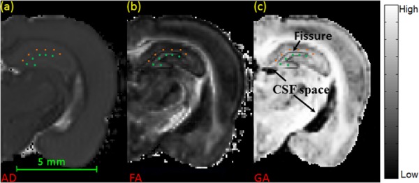
MR images of rat brain. (a) AD map of a coronal brain slice (background was set to be black). (b) FA map of a coronal brain slice. (c) GA map of the same slice, with improved contrast between CSF and WM. Squares indicate the location of lacunosum-moleculare layer and circles indicate the location of molecular layer.
2.2. Tissue Segmentation and Fissure Assignment.
The image segmentation process was performed through a semi-automatic methodology based on a custom matlab subroutine (matlab v.R2012a, Mathworks, Natick, MA). AD was used first to segment between tissue and CSF space regions, as the AD value in biological tissue is notably smaller than that in fluid space. Then, the FA value was employed to segment most regions of WM and GM in the brain, as the FA value directly reflects the extent of tissue alignment in each imaging voxel. Usually, WM has a higher FA value than GM [37]. To improve segmentation in complex tissue structures such as the hippocampus where crossing fibers are present, the hippocampus region was manually isolated slice by slice using a matlab subroutine. GA values were then used to segment WM and GM in these regions. Thresholds for AD, FA, and GA were adjusted using visualization software (amira v.4.1, TGS, San Diego, CA) and determined by making segmented regions match a rat brain atlas [38,39]. Final threshold values are listed in Table 1.
Table 1.
Thresholds used for segmentation of tissue volumes
| Regions | Range |
|---|---|
| CSF space | η to 1 |
| WM | δ or ε to 1 |
| GM | 0 to δ or ε |
| MRI data | Thresholds |
|---|---|
| Normalized AD (η) | 0.356 |
| FA (δ) | 0.294 |
| GA (ε) | 0.877 |
Since fissures and CSF are fluid filled regions, GA values were low compared to surrounding tissues. These regions were clearly seen as dark regions on GA maps and fissures could be traced out manually within the hippocampus. Fissure and CSF regions were also checked by comparing them to a rat atlas [38,39]. Figure 2(b) shows segmentation of fissures in the dorsal and ventral hippocampus based on GA. These are used to generate computational hippocampal fissure (HF) models. For computational models with no hippocampal fissures (NHF), fissures were not manually traced or labeled. Otherwise, the NHF model was developed similarly to the HF model; segmentation was based on FA and GA and these regions ended up as mostly GM though some fluid spaces may be present. Figure 2(a) shows the final segmentation used in the voxelized model. For the HF model, the goal was to generate connected fluid-filled spaces between fissures and other CSF spaces such as ventricles. The 3D structure of the lateral ventricles shown in Fig. 3 was used to visualize connected CSF space.
Fig. 2.
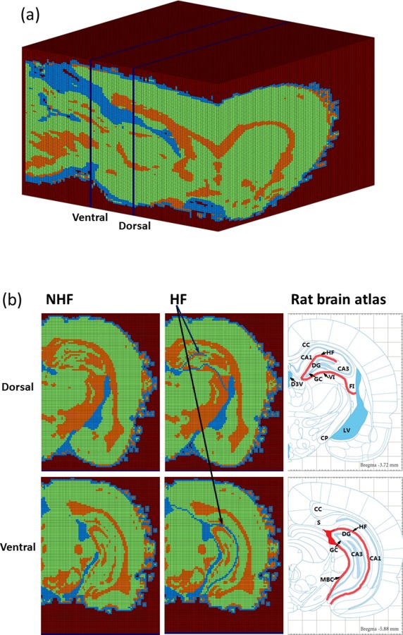
Segmented brain volume: (a) voxelized brain model (impermeable regions, GM, WM, and CSF spaces); (b) segmentation of dorsal and ventral hippocampi slices without hippocampal fissures (NHF) and with fissures (HF). Atlas figures show location of fissures and CSF in thick lines. Labels indicate the location of the CA1, CA3, corpus callosum (CC), cerebral peduncle (CP), dorsal 3rd ventricle (D3V), dentate gyrus (DG), fimbria (FI), granule cell layer (GC), hippocampal fissure (HF), lateral ventricle (LV), midbrain cistern (MBC), subiculum (S), and velum interpositum (VI).
Fig. 3.
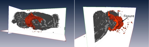
Three-dimensional structure of the fluid-filled lateral ventricles. The fluid-filled space was shown as the bulge part along the sagittal tissue slice. Fissures connected to ventricles and other CSF spaces are also shown.
The CED infusion sites of our previous experimental studies were reported based on stereotactic location [17]. In order to find these locations with our segmented brain maps, we compared anatomical structures visible on the GA map with the given stereotactic location in the rat brain atlas [39]. The infusion site was assigned as a single voxel in our segmented brain maps.
2.3. Flow Transport Model.
A voxelized modeling approach to simulate CED flow and drug transport in brain has been previously developed by our group [9,13,22]. A brief description follows. A more detailed description of this voxelized model procedure and its assumptions can be found in the following papers [13,22]. The major difference of this study is an improved segmentation method that employs GA to identify crossing fiber regions.
2.3.1. Porous Media Transport.
Extracellular transport in brain tissue was modeled assuming tissue as rigid porous media. This assumption is valid when the infusion rate is low and pressure during infusion in tissue is small, or if the initial deformation occurs over a much shorter time scale than CED infusion time. Perivascular transport was not accounted for in this CED model, but has been sometimes observed in infusion into the rat hippocampus [16]. In porous media, the continuity of fluid equation is
| (3) |
where is the volume averaged extracellular fluid velocity in tissue, and β is a volumetric flow rate source term for the endogenous fluid flow in brain tissue which is estimated to be 0.3 mg/min cm3 [40]. The governing equation for porous media is Darcy's law
| (4) |
where p is pore pressure and K is the hydraulic conductivity. Darcy's law was also applied to fluid regions, like CSF spaces and subarachnoid spaces in the model. This assumption lumps boundary layer and viscous effects into the hydraulic conductivity value. The convection-diffusion equation is the principal equation for transport in porous media
| (5) |
where ϕ is the tissue porosity, t is time, is the normalized concentration, and D is the tracer diffusivity in WM, GM, or CSF space. In this study, ϕ = 0.26 in brain tissue, which is the value previously estimated in CED studies on the spinal cord of rat [41,42]. In CSF regions, porosity ϕ was set to 1. For CED, the site of infusion was modeled as a single voxel source in which constant velocity and concentration () was applied at wall boundaries of the voxel.
2.3.2. Tissue Transport Properties.
In GM and CSF, the hydraulic conductivity and diffusion properties were isotropic. In WM, these transport properties were anisotropic and assumed to have the same principal directions as the water diffusion tensor De. The preferential direction (direction of maximum transport) was assumed to be the same as the eigenvector direction of the largest principle eigenvalue of De. The other two eigenvector directions perpendicular to the fiber direction were treated as transversely isotropic. The tissue properties used for extracellular transport are listed in Table 2. In each voxel of WM, the hydraulic conductivity tensor K and tracer diffusion coefficient D can be calculated
Table 2.
Tissue properties used in simulation
| (6) |
| (7) |
where are eigenvectors of water diffusion De acquired from diffusion tensor imaging with the eigenvector based on the largest eigenvalue λ1. Kǁ and are eigenvalues of K; Dǁ and are eigenvalues of , where and subscripts indicate parallel and perpendicular directions with respect to the WM track. Values are listed in Table 2. By using this formulation, the direction of preferential transport varies in each voxel according to the fiber direction assigned by De.
Governing fluid transport equations (3)–(5) were solved using the computational fluid dynamic package, fluent (ansys 13, ANSYS, Inc. Canonsburg, PA). A cuboid mesh, whose cell size was the same as the voxel size, was created for simulation in gambit (anasys 13, ANSYS, Inc. Canonsburg, PA). Since the left and right hemispheres of the brain are approximately symmetric, the simulation was only performed on half of the brain to reduce computation time, and symmetry boundary conditions were applied along the central sagittal plane. The pore pressure and normalized concentration were set to zero at all the other outside boundaries. A user-defined subroutine was used to assign K and D to each simulation cell based on Eqs. (6) and (7). There were two steps to solve CED tracer transport. First, constant velocity was applied to each wall of the infusion voxel to solve for the steady flow field due to CED based on Eqs. (3) and (4). Then, the CED tracer distribution in tissue was predicted by solving the convection–diffusion equation (Eq. (5)) under this flow field. Postimage processing was done with matlab and an open-source medical image segmentation software itk-snap [44]. A tissue concentration value of 5% of the maximum concentration was used as the cut-off threshold in distribution calculations. This is the same value used in previous studies by our group [13,22]. Tracer distribution area was calculated to measure tracer distribution area within a single image slice. Tracer distribution volume calculated tracer volume using multiple image slices. Both tracer distribution area and volume calculated tracer spread into tissue, fissure, and CSF regions of the brain.
2.3.3. CED Parameters.
In models with and without fissures, CED distributions were simulated at two infusion sites: dorsal hippocampus (AP:-3.7, ML:2.2, DV:-2.75) and ventral hippocampus (AP:-5.88, ML:5.1, DV:-5.5). The infusate was albumin tracer, and CED infusions were at a rate of 0.3 μl/min. Albumin is a nonbinding and nonreacting macromolecule (molecular weight = 66.5 kDa). It stays mainly in the extracellular space, so it is commonly used in tracer studies.
2.3.4. Parameter Analysis.
Even though ventricles and fissures are fluid-filled regions, an equivalent porous media hydraulic conductivity value was used for flow and tracer simulations. To estimate hydraulic conductivity of CSF (KCSF), we initially assumed flow in fissures was equivalent to flow between parallel plates. Analytical solutions for this flow were used to estimate the order of magnitude of KCSF. As the average velocity of parallel flow is expressed as
| (8) |
where h is the height of the fissure, and μ is the viscosity of infusate and interstitial fluid. Hence, compared with Darcy's law (Eq. (4)), the equivalent permeability for fissure regions, , was estimated to be
| (9) |
The viscosity of water at 35 °C is 7.225 × 10⁻⁴ Pa·s. Since fissure features are small, we initially assumed height to be equivalent to dimension of a single voxel (h = 0.095 mm) as segmented in our GA map (Fig. 1(c)). This assumption overestimates the fissure height; thus, the calculated KCSF_EST provides an upper bound value. Using this value, KCSF_EST/KWMǁ = 1.54 × 10⁵ showing that fissures provide much less resistance to flow than GM. To determine the sensitivity of the model to KCSF, CED simulations were conducted for varying ratio of KCSF/KWMǁ between 10, 102, 103, 104, and 105. These smaller ratios essentially assume smaller fissure heights and greater resistance to flow within the fissure.
2.4. Comparison of Distribution Patterns With Experimental CED Studies.
Experimental CED studies of infusion into the ventral and dorsal hippocampus of rat brain have previously been conducted by our group [17,32]. In these studies, 5–10 μl of Gd-albumin with Evans Blue at 0.3 μl/min was infused to provide MR quantitation of in vivo distribution patterns. In the earlier study by Kim et al. [32], both dorsal and ventral infusions were measured while the animal was in the magnet. In the study by Astary [17], in vivo concentration profiles were calculated using measured relaxivities with DCE-MRI through equations describing signal intensity to the contrast agent concentration [45]. Computational simulations used the same stereotaxic infusion locations and infusion rates for albumin tracer. Distribution patterns and areas of distribution along coronal planes were compared.
Computational models were based on MRI data from fixed rat brains. Since fixed tissues shrink due to cross-linking [30,46], model predictions may underestimate distribution area. Calculated CED distribution areas can be modified to account for tissue dimensions that shrink in order to compare with in vivo, CED distribution experimental data. This normalization was based on brain width. The widest part of the brain was determined for fixed brains and brains from in vivo MRI scans. Ten in vivo rat brains (average width = 15.62 ± 0.292 mm) and five fixed brains widths (average width = 15.06 ± 0.0793 mm) were measured to examine brain shrinkage. (Height was not as easily comparable due to changes in brain shape with removal from the skull.) This width change ( + 3.75%) was used to modify the simulated distribution areas (+7.64%) and distribution volumes (+11.7%) when comparing to in vivo values. These values are similar to previously reported studies of tissue shrinkage. In a MR mouse atlas study, the outside hippocampus surface area was reported to be reduced by 6.9% [30] (corresponding to a + 7.41% distribution area change) and hippocampus volume was reduced by 11.6% [30] (corresponding to + 13.12% distribution volume change).
3. Results
3.1. Segmentation of Rat Brain.
Figure 2 shows the whole brain with (HF) and without specific segmentation of hippocampal fissures (NHF). WM, GM, and CSF volumetric percentages were 21.1%, 64.8%, and 14.1%, respectively, in the HF model with segmented, continuous fissures. These percentages changed slightly to 21.1%, 65.3%, and 13.6%, respectively, in the NHF model. With inclusion of continuous fissures, the percentage of CSF only increased by approximately 0.5%. However, greater connectivity of fluid spaces was achieved model compared to NHF model. In the HF model, the hippocampal fissure connected to the third ventricle in the dorsal hippocampus; the hippocampal fissure connected to the midbrain cistern and subarachnoid space in the ventral hippocampus. In the NHF model, the ventricle system (ventricles, subarachnoid) and the midbrain cistern were also segmented. However, the hippocampal fissure was not assigned as CSF. Hence, in the NHF model, there was less of a fluid pathway connection between the lateral ventricle and third ventricle in the dorsal hippocampus and between the ventricle system and the midbrain cistern in the ventral hippocampus.
3.2. Hydraulic Conductivity Sensitivity Analysis.
CSF conductivity influences the diversion of CED tracer into CSF spaces. Predicted CSF distribution volumes for different KCSF/KWMǁ are shown in Fig. 4. For varying CSF hydraulic conductivity, there was little change in CSF distributions over a large range of KCSF/KWMǁ from 102 to 105, indicating low sensitivity of the model within this range. The upper limit of CSF conductivity was bounded by the estimated permeability from parallel plate analysis (KCSF_EST/KWMǁ ∼ 105). For lower values of CSF conductivity (KCSF_EST/KWMǁ = 10), distributions were not as likely to enter CSF regions and tissue distributions were greater. This same pattern was maintained for both dorsal and ventral infusion sites. Given these results, (KCSF_EST/KWMǁ = 102) was used, in the remainder of simulations.
Fig. 4.
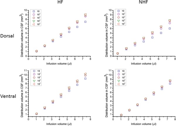
Albumin tracer distribution volumes in CSF after CED. (Left) Simulations with hippocampal fissures and (right) no fissures for varying infusion volumes in (top) dorsal and (bottom) ventral hippocampus. The hydraulic conductivity of CSF ranged as KCSF/KWMǁ from 10 to 105.
A sensitivity study was also performed increasing the tissue hydraulic conductivity values overall. More recent models have used higher conductivity values [47] and this allowed us to determine the influence of higher values on model results. KGM, KWM∥, KWM⊥, and KCSF were increased by 1 order of magnitude (see Table 2). CED distribution volume changed less than 4% and distribution patterns changes were also small. This is consistent as long as hydraulic conductivity ratios, e.g., KGM/KWM, remain the same. However, CED infusion pressure was found to decrease proportionally by approximately 1 order of magnitude (see Table 3). Thus, the magnitude of the hydraulic conductivity influences predicted pressure fields and can be changed to better match infusion pressure measurements [47]; however, CED distribution properties are not greatly affected.
Table 3.
Pressure at infusion sites within the dorsal and ventral hippocampi. Simulations were for an infusion rate of 0.3 μl/min. Low K model uses K values in Table 2. High K model uses values which are 1 order of magnitude higher than K values in Table 2.
| Infusion pressure | HF | NHF | |
|---|---|---|---|
| Low K | Dorsal | 76.2 kPa | 86.3 kPa |
| High K | (7.62 kPa) | (8.63 kPa) | |
| Low K | Ventral | 96.2 kPa | 97.8 kPa |
| High K | (9.62 kPa) | (9.78 kPa) | |
3.3. Predicted Tracer Distribution Volume.
Steady-state extracellular fluid fields were simulated during CED infusion. The predicted pressures at the infusion site (cannula needle tip) are listed in Table 3. In both dorsal and ventral hippocampi, the infusion pressure decreased with the introduction of fissures, −11.7% in dorsal and −1.64% in ventral.
Simulated CED tracer distribution volumes within the brain are shown in Fig. 5. With increasing infusion volume, brain tissue distribution volume was nearly linear for both dorsal and ventral hippocampi infusion sites. Ratios for tissue distribution to infusion volume (Vd/Vi) are listed in Table 4. When fissures were included, the final distribution volume in the whole brain decreased. The ratio of distribution volume in CSF to infusion volume (Vd_CSF/Vi) was also approximately linear and is shown in Fig. 4. This ratio increased with the inclusion of fissures (see Table 4).
Fig. 5.
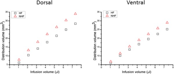
Albumin tracer distribution volumes in the brain (tissue and CSF) after CED. Tracer distribution volume in (left) dorsal and (right) ventral hippocampus for an infusion rate of 0.3 μl/min for fissures (HF) and no fissures (NHF).
Table 4.
Volume distribution ratios for brain tissue (Vd/Vi) and CSF (Vd_CSF/Vi) for CED into the dorsal and ventral hippocampus
| HF | NHF | |
|---|---|---|
| Vd/Vi a | ||
| Dorsal | 3.74 | 4.48 |
| Ventral | 3.29 | 3.79 |
| Vd_CSF/Vi | ||
| Dorsal | 1.18 | 1.00 |
| Ventral | 1.37 | 1.19 |
Slope of distribution volume versus infusion volume in Fig. 5.
In simulations, infused tracer initially distributed into adjacent tissues. When infusate encountered a fissure or CSF space, it then would preferentially flow into these lower resistance regions. Varying CED tracer distributions between different tissue regions (WM, GM, and CSF) are shown in Fig. 6. For both dorsal and ventral infusions, distributions are initially within WM and GM. As expected with increasing infusion, a greater portion of the infusate is diverted to CSF. For dorsal CED, approximately 9.5% greater CSF distribution was predicted in models with fissures compared to models without fissures. Also, comparing models with and without hippocampal fissure for ventral CED, 6–10% more infusate diverted to CSF with fissures; this percentage increased with increasing infusion volume. Comparing ventral to dorsal CED, 6% more tracer was diverted to CSF during ventral infusion with increasing infusion volume in the HF model.
Fig. 6.
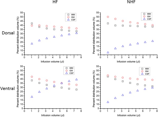
Simulated infusate distribution volume in different tissue regions for CED in dorsal and ventral hippocampus. (Left) Volume percentage of tracer in WM, GM, and CSF in HF model. (Right) Volume percentage of tracer in WM, GM, and CSF in NHF model. (Top) In dorsal hippocampus and (bottom) in ventral hippocampus. The infusion rate was 0.3 μl/min.
3.4. CED Distribution Patterns and Comparison With Experimental CED Studies.
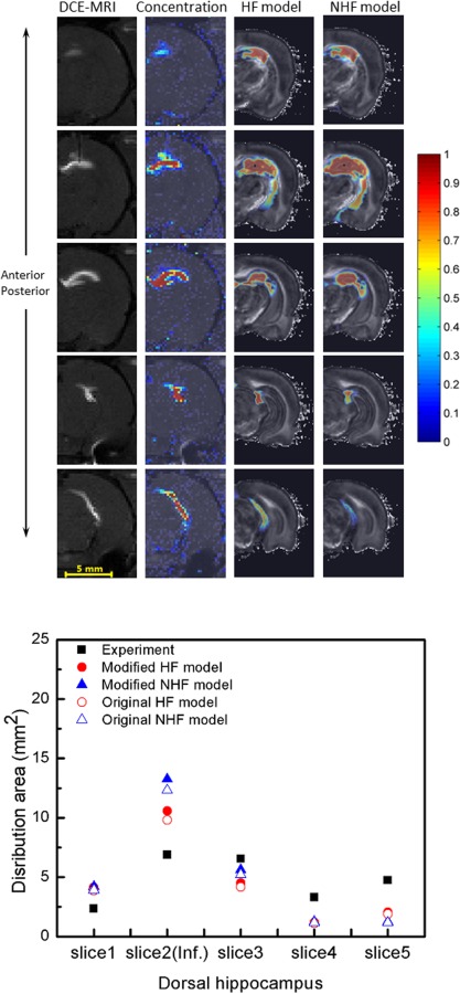
Simulated tracer CED distributions were compared with in vivo distributions from our previous DCE-MRI studies [17]. First, distribution patterns from simulations were compared with MRI distributions. Figures 7 and 8 show tracer penetration in the anterior–posterior direction, and distribution in hippocampus and surrounding regions. For both dorsal and ventral hippocampal infusion sites, predicted albumin tissue distributions show similar regional patterns to what was previously measured. Tissue concentration maps predicted by the HF model captured tracer distribution further into anterior–posterior directions when compared with the MR measurements. As shown in the fifth row in Figs. 7 and 8, there was more tracer distribution into the midbrain cistern in the HF model than in the NHF model. In simulations of infusion into the dorsal hippocampus, tissue distributions in the HF model more closely matched concentration contours from experiments since these predicted smaller tissue spread than the NHF model because of the inclusion of a fissure. For the ventral hippocampus infusion site, tracer spread was smaller in the HF model as it has more leakage into the midbrain cistern, and captured less distribution than DCE-MRI measurements.
Fig. 7.
Comparison of experimentally measured DCE-MRI distributions with predicted CED into the dorsal hippocampus. (Top) DCE-MRI measured distribution (column 1) and measured concentration profiles (column 2) with simulated tracer distributions from the HF model (column 3) and the NHF model (column 4). Different rows show concentration contours from anterior to posterior regions. Albumin of 7.35 μl (and Gd-albumin) tracer was infused at 0.3 μl/min. (Bottom) Comparison of tracer distribution area calculated in consecutive MR imaging slices. Area spread is based on a 5% normalized concentration () threshold. Filled triangles and circles show an adjusted distribution range that accounts for tissue shrinkage in the model geometry (+7.64%).
Fig. 8.
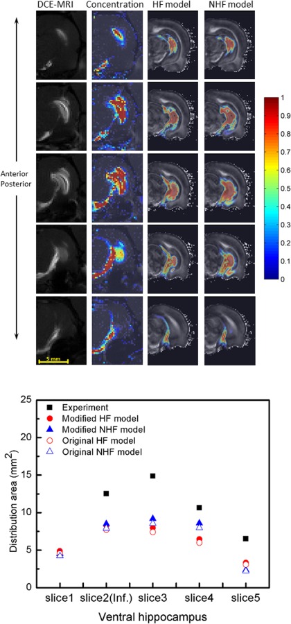
Comparison of experimentally measured DCE-MRI distributions with predicted CED into the ventral hippocampus. (Top) DCE-MRI measured distribution (column 1) and measured concentration profiles (column 2) with simulated tracer distributions of HF model (column 3) and NHF model (column 4) through concentration contour for infusions into ventral hippocampus form anterior to posterior in rows. CED of 7.35 μl of albumin (and Gd-albumin) tracer was infused at 0.3 μl/min. (Bottom) Comparison of tracer distribution area calculated in consecutive MR imaging slices. Area spread is based on a 5% normalized concentration () threshold. Filled triangles and circles show an adjusted distribution range that accounts for tissue shrinkage in the model geometry (+7.64%).
At the infusion slice, predicted tracer distributions (concentration contours) in the dorsal hippocampus are shown in Fig. 9. Tracer remained in the hippocampus for small infusion volumes (<3.15 μl). With increasing infusion volume, tracer reached boundaries of the hippocampus and fissures. In the dorsal hippocampus, the infusion site was approximately 0.29 mm to the hippocampal fissure and 0.38 mm to the velum interpositum. Once this occurred, infusate appeared to track along regions adjacent to fissures in the lateral ventricle. Tracer was diverted into fissures where it distributed into these spaces, was diluted, and was able to access larger CSF spaces. So, tissue distribution in models with fissures was smaller compared to models without fissures. In simulations without specifically defined fissures, there was greater overall tissue penetration with tracer reaching as far as cerebral peduncle regions.
Fig. 9.
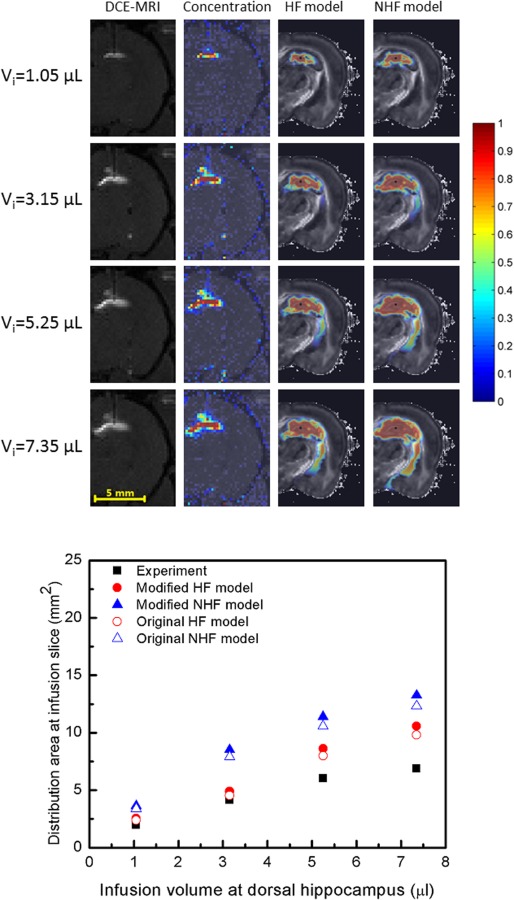
CED distribution of albumin tracer in dorsal hippocampus with increasing infusion volume. (Top) DCE-MRI measured distribution (column 1) and measured concentration profiles (column 2) with simulated tracer distributions of HF model (column 3) and NHF model (column 4) for varying infusion volumes: (row 1) Vi = 1.05 μl, (row 2) Vi = 3.15 μl, (row 3) Vi = 5.25 μl, and (row 4) Vi = 7.35 μl. Infusions were at 0.3 μl/min. (Bottom) Comparison of tracer distribution area calculated in the infusion slice of the dorsal hippocampus. Area spread is based on a 5% normalized concentration () threshold. Filled triangles and circles show an adjusted distribution range that accounts for tissue shrinkage in the model geometry (+7.64%).
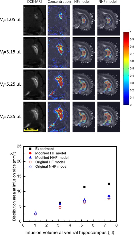
For CED in the ventral hippocampus, a similar tissue diversion pattern was observed (see Fig. 10). Tracer reached fissures in the midbrain cistern region where it was diverted to fissures. Without fissures, greater tissue penetration was again predicted with tracer reaching ventral subiculum regions. For simulation in ventral hippocampus, the infusion site was ∼0.38 mm to the hippocampal fissure and ∼0.95 mm to the midbrain cistern.
Fig. 10.
CED spread of albumin tracer into the ventral hippocampus with increasing infusion volume. (Top) DCE-MRI measured distribution (column 1) and measured concentration profiles (column 2) with simulated tracer distributions of HF model (column 3) and NHF model (column 4) for varying infusion volumes: (row 1) Vi = 1.05 μl, (row 2) Vi = 3.15 μl, (row 3) Vi = 5.25 μl, and (row 4) Vi = 7.35 μl. Infusions were at 0.3 μl/min. (Bottom) Comparison of tracer distribution area calculated in the infusion slice of the ventral hippocampus. Area spread is based on a 5% normalized concentration () threshold. Filled triangles and circles show an adjusted distribution range that accounts for tissue shrinkage in the model geometry (+7.64%).
The mean absolute difference was used to compare distribution areas of HF and NHF model results to experimental results (Figs. 7–10), see Table 5. The mean absolute difference was calculated by averaging the absolute difference of the simulation result (predicted distribution area) and the experimental result (measured area) across all slices using data in the bottom graphs of Figs. 7–10. For the dorsal CED model, the mean absolute difference in the HF model was smaller than the NHF model. In the ventral CED model, the mean absolute difference in the HF model was slightly higher than in the NHF model. Distribution volumes from in vivo DCE-MRI [17] (Figs. 7 and 8) that were captured in five coronal slices were estimated and compared to our computational models over the same region, as shown in Fig. 11. Linear interpolation was used to reduce the slice thickness of in vivo MRI scans from 1 mm to 0.25 mm. The distribution volume was estimated by summing the segmented distribution areas multiplied by the thickness of each slice. In the dorsal hippocampus, the distribution volume of the HF model more closely matched in vivo distribution volume. In the ventral hippocampus distribution volumes of HF and NHF models were similar and underestimated the in vivo estimate.
Table 5.
Mean absolute difference of distribution area of HF and NHF models compared to experimental data
| Mean absolute difference (mm2) | HF | NHF | |
|---|---|---|---|
| Dorsal | Slices (anterior–posterior) | 2.47 | 2.94 |
| Infusion slice | 1.91 | 4.44 | |
| Ventral | Slices (anterior–posterior) | 3.78 | 3.19 |
| Infusion slice | 2.57 | 2.28 | |
Fig. 11.
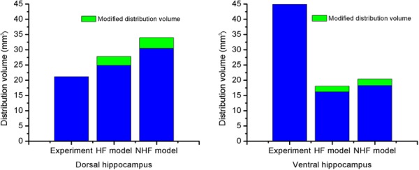
Comparison of calculated distribution volumes in a region after the end of CED into the dorsal (left) and ventral (right) hippocampus. Results from HF and NHF models are long bars. Adjusted distribution volumes are short bars stacked on top (+11.7%).
4. Discussion
MR-based, computational models have the potential to improve predictions of drug coverage and provide more accurate surgical planning. In clinical trials of CED, there are some rules of thumb used to plan the location of the infusion site to optimize targeting. The goal is to avoid leakage to fissures, ventricles, subarachnoid regions, and WM. For example, the needle tip should be placed more than 3 cm to the brain surface and more than 1 cm to ventricles [2]. Thus, it is well-known that tissue-fluid boundaries play an important role in flow diversion during infusion. In previous CED modeling studies, fissures have not been included since they are small scale features that are not easily resolved with MR. Hippocampal fissures are fetal sulcus around which the hippocampus folds during brain development. They are important in that they may divert flow during infusions and provide an interconnected channel to ventricles. In this study, we have included fissure spaces through an improved segmentation scheme and conducted comparative studies to better determine the role of fissures during infusions. Moreover, the neuroanatomical structure of the rat dorsal hippocampus region was also segmented. We compared model simulations with previously acquired MR measures of tracer spread by our group [17]. Comparisons with MR tracer spread were also improved by using DCE-MRI to quantify in vivo concentrations.
4.1. Tissue Segmentation.
We have provided an improved segmentation method that utilizes GA to account for the complex tissue composition and embedded fissure structures within the hippocampus. In previous CED brain and models [48], as well as studies by other groups, fissures are often omitted due to their small scale, which is difficult to differentiate with MR. As a result, CSF spaces are generally smaller and less connected in these previous models. GA is calculated from a higher order tensor (four or six-rank), and is able to delineate crossing fiber structures constituting tissue, as it accounts for multidirectional tissue fibers in a voxel. Because of this, it better labels WM tissues and provides higher contrast of tissues surrounding fluid only regions than when using FA (two-rank) which is only able to capture one direction of alignment. The low GA regions (dark regions) matched well with fissure boundaries mapped in rat atlases [39].
4.2. CED Model Predictions.
The fissure space is an important fluid boundary in CED simulations. It acts as a low fluid resistance sink where fluid, tracers, and drugs are preferentially diverted. In this study, we determined the effect of changing fissure geometry and properties on CED diversion. The HF model was able to capture hippocampal fissure connectivity. In the dorsal hippocampus, the hippocampal fissure is connected to the third ventricle [39], and in the ventral hippocampus, the hippocampal fissure is connected to the ambient cistern and interpeduncular cistern [49]. These cisterns belong to the ventricle system. Fissures have high fluid conductivity and only by artificially decreasing KCSF to a low value (KCSF/KWMǁ < 102) were CED distributions affected. Based on the segmentation method in this study, the fissure size was segmented to be the same to the voxel size (0.095 mm). The actual fissure may not be this size, and may be smaller.
The segmented fissures were better connected to ventricle spaces, providing more physiologically realistic flow connectivity than models that were less connected. The HF models predicted lower infusion pressures than the NHF models. This is likely due to access to a lower resistance flow pathway created by the connected fissures. The corresponding CED tissue distributions decreased in the HF models since more infusate was diverted to CSF. Between 6% and 10%, more infusate was diverted into CSF in the HF model compared to the NHF model. It is expected that this percentage would increase with increasing infusion volume. These CED diversion effects are consistent with our previous CED tracer studies [16,17,32] where hyperintense regions were observed within and surrounding the hippocampal fissure in MR imaging, and high concentration of dye at the fissure surface was also shown in histological images. Also, the final CED distribution volume ratios decreased 16.5% in the dorsal hippocampus and 13.2% in the ventral hippocampus when fissures were accounted for in the model. This result was in accord with previous experimental observations by other groups, which reported there was a decrease in slope of Vd/Vi after imaging tracer crossed ventricular and pial surfaces [15] and there was leakage into ventricles and sulci during CED [18]. The HF model in this study is to the best of our knowledge the first to simulate the effect of these tiny fluid boundaries. The results of this study show that fissures affect the transport of drug agents during CED. Thus, it is important to consider the position of infusion cannulas with respect to these fluid pathways when planning surgical treatment.
4.3. Experimental Comparison.
We have quantified tracer concentration through DCE-MRI using previously measured relaxivity values [17]. These data enable comparison of our simulated concentration distributions with in vivo MR tracer studies. In the dorsal hippocampus, CED infusate transports mainly in medial–lateral and anterior–posterior directions; in the ventral hippocampus, the infusate transports mainly in inferior–superior and anterior–posterior directions [32]. The inclusion of fissures resulted in capturing these general distribution patterns and provided better anterior to posterior coverage for both dorsal and ventral infusion sites (Figs. 7 and 8).
Overall, inclusion of fissures (HF model) captured CED at the dorsal site better than the model without fissures (NHF) when comparing to experimental data. This was true when comparing distribution areas across slices as well as with increasing infusion volume within the same slice (Fig. 9). The distribution volumes were better matched using the HF model (in Fig. 11).
For the ventral infusion site, CED predictions for the HF and NHF models were not substantially different from each other (Fig. 10). Predicted distribution volumes in ventral hippocampus were also compared quantitatively with our previously collected experimental data. The predicted distribution volume in ventral hippocampus was found to be smaller (only 60% for HF and NHF models) when compared to the DCE-MRI CED measurement, which was an underprediction. In previous CED modeling studies by our group, Kim et al. also modeled infusion into the ventral hippocampus [22]. These previous studies seemingly are able to better capture the distribution pattern and volume (42 mm3) seen in the MR CED measurement even though these models did not include the hippocampal fissure. (CED into the dorsal hippocampus was not predicted in the Kim et al. study [22] since the dorsal hippocampus did not provide enough contrast to separate WM, GM, and CSF.) There were several reasons that may explain discrepancy of our ventral CED model results from this previous study. (1) One reason is interanimal variability and differences in CSF space. In the current model, there is more segmented CSF space (13.6% versus 11.1%) that acts as a fluid sink during CED resulting in smaller predicted distribution volume. (2) There was also difference in location of the infusion site. The cannula tip position in the Kim et al. study [22] was in CA1, and was lateral to the hippocampal fissure. In the current study, the cannula tip position was in the DG, and was medial to the hippocampal fissure. In addition, the distance of the infusion site to the midbrain cistern (a common CSF sink) in the Kim et al. study [22] was 1.5 mm; in this study, it was less (0.95 mm); and in the DCE-MRI CED experiment [17], it was 1.25 mm. If we used the same distance to the midbrain cistern as measured in the MR of the CED experiment, the infusion site in the computational model would have been outside of the DG and in the CA1. Consequently, the simulated CED tracer resulted in more fluid and tracer diversion to penetrate the midbrain cistern. (3) Finally, another reason for discrepancy of ventral CED distributions is tissue shrinkage from fixation which resulted in smaller brain tissue volumes and larger CSF regions in the computational model. In the ventral hippocampus, simulation errors may increase as the fissure volume is overpredicted and the midbrain cistern is enlarged. This would also result in an overprediction of leakage into CSF spaces and underprediction of CED tissue distribution volume by the computational model. In our current study, it should be emphasized that CSF diversion during CED seemed to be most affected by the relative infusion site location to the midbrain cistern, and this is likely the main reason that predictions to this region were underpredicted in the ventral location and predicted CED in other regions like the dorsal hippocampus were not.
It should be noted that brain structure can vary between animals, and the simulated distribution predicted using fixed animal brains may differ from in vivo data collected in another animal. While simulation results captured the major drug distribution properties in the rat brain, structural and volumetric differences of the model rat brain may be a source of error. Collection of in vivo DWI data would provide further validation on an individual rat basis. In addition, the model is on a small rat brain. Transport equations (conservation and momentum) relations may be scaled to larger patient scales using the same tissue transport properties assuming approximately similar extracellular tissue structure across species.
5. Conclusion
While the role of the ventricle system in CED diversion is well known, the effect of smaller fluid spaces has been less studied. During the clinical application of CED, these spaces can affect therapeutic agent distributions. It is important to consider the position of infusion cannulas with respect to these fluid pathways when planning surgical treatment. In this study, a voxelized model based on MRI data was adapted to account for hippocampal fissures. The developed models are to the best of our knowledge the first to account for CED diversion into fissure spaces. Thus, computational tools that can be used to predict effect of varying infusion sites would be useful to optimize treatment over specific target regions while avoiding leakage to other places. Simulated CED distribution results were compared with the concentration data from MR tracer experiments. The models that included hippocampal fissures matched well with DCE-MRI patterns measured in the dorsal hippocampus. In the ventral hippocampus, CED models only captured ∼60% of the measured distribution volume. The likely reason for this was due to infusion site placement and tissue volume shrinkage that varied between the model and experiments. The quantitative methodology developed in this study shows a way forward for further validation of the voxelized CED model.
Acknowledgment
We would like to thank Dr. Luis Perez who collected the fixed rat brain DWI data. All the MRI data in this study were obtained at the Advanced Magnetic Resonance Imaging and Spectroscopy Facility in the McKnight Brain institute and National High Magnetic Field laboratory of UF. This work was funded by NIH R01NS063360.
Contributor Information
Wei Dai, Department of Mechanical and , Aerospace Engineering, , University of Florida, , Gainesville, FL 32611 , e-mail: weidai@ufl.edu.
Garrett W. Astary, J. Crayton Pruitt Family , Department of Biomedical Engineering, , University of Florida, , Gainesville, FL 32611 , e-mail: gwastary@gmail.com
Aditya K. Kasinadhuni, J. Crayton Pruitt Family , Department of Biomedical Engineering, , University of Florida, , Gainesville, FL 32611 , e-mail: adityakumar.bme@gmail.com
Paul R. Carney, Department of Neuroscience, , Department of Pediatrics, , Division of Pediatric Neurology, , J. Crayton Pruitt Family , Department of Biomedical Engineering, , Wilder Center of Excellence , for Epilepsy Research, , University of Florida, , Gainesville, FL 32611 , e-mail: carnepr@peds.ufl.edu
Thomas H. Mareci, Department of Biochemistry , and Molecular Biology, , University of Florida, , Gainesville, FL 32611 , e-mail: thmareci@ufl.edu
Malisa Sarntinoranont, Department of Mechanical , and Aerospace Engineering, , University of Florida, , MAE A 212, , Gainesville, FL 32611 , e-mail: msarnt@ufl.edu.
References
- [1]. Longo, D. L. , Fauci, A. S. , Kasper, D. L. , Hauser, S. L. , Jameson, L. , and Loscalzo, J. , 2012, Harrison's Principles of Internal Medicine, McGraw-Hill, New York. [Google Scholar]
- [2]. Sampson, J. H. , Brady, M. L. , Petry, N. A. , Croteau, D. , Friedman, A. H. , Friedman, H. S. , Wong, T. , Bigner, D. D. , Pastan, I. , Puri, R. K. , and Pedain, C. , 2007, “ Intracerebral Infusate Distribution by Convection-Enhanced Delivery in Humans With Malignant Gliomas: Descriptive Effects of Target Anatomy and Catheter Positioning,” Neurosurgery, 60(2), pp. 89–98. 10.1227/01.NEU.0000249256.09289.5F [DOI] [PubMed] [Google Scholar]
- [3]. Fiandaca, M. S. , Forsayeth, J. R. , Dickinson, P. J. , and Bankiewicz, K. S. , 2008, “ Image-Guided Convection-Enhanced Delivery Platform in the Treatment of Neurological Diseases,” Neurotherapeutics, 5(1), pp. 123–127. 10.1016/j.nurt.2007.10.064 [DOI] [PMC free article] [PubMed] [Google Scholar]
- [4]. Parekh, M. B. , Carney, P. R. , Sepulveda, H. , Norman, W. , King, M. , and Mareci, T. H. , 2010, “ Early MR Diffusion and Relaxation Changes in the Parahippocampal Gyrus Precede the Onset of Spontaneous Seizures in an Animal Model of Chronic Limbic Epilepsy,” Exp. Neurol., 224(1), pp. 258–270. 10.1016/j.expneurol.2010.03.031 [DOI] [PMC free article] [PubMed] [Google Scholar]
- [5]. Kantorovich, S. , Astary, G. W. , King, M. A. , Mareci, T. H. , Sarntinoranont, M. , and Carney, P. R. , 2013, “ Influence of Neuropathology on Convection-Enhanced Delivery in the Rat Hippocampus,” PLoS One, 8(11), p. e80606. 10.1371/journal.pone.0080606 [DOI] [PMC free article] [PubMed] [Google Scholar]
- [6]. Allard, E. , Passirani, C. , and Benoit, J.-P. , 2009, “ Convection-Enhanced Delivery of Nanocarriers for the Treatment of Brain Tumors,” Biomaterials, 30(12), pp. 2302–2318. 10.1016/j.biomaterials.2009.01.003 [DOI] [PubMed] [Google Scholar]
- [7]. Rosenbluth, K. H. , Eschermann, J. F. , Mittermeyer, G. , Thomson, R. , Mittermeyer, S. , and Bankiewicz, K. S. , 2012, “ Analysis of a Simulation Algorithm for Direct Brain Drug Delivery,” Neuroimage, 59(3), pp. 2423–2429. 10.1016/j.neuroimage.2011.08.107 [DOI] [PMC free article] [PubMed] [Google Scholar]
- [8]. Wolak, D. J. , and Thorne, R. G. , 2013, “ Diffusion of Macromolecules in the Brain: Implications for Drug Delivery,” Mol. Pharmaceutics, 10(5), pp. 1492–1504. 10.1021/mp300495e [DOI] [PMC free article] [PubMed] [Google Scholar]
- [9]. Sarntinoranont, M. , Chen, X. , Zhao, J. , and Mareci, T. H. , 2006, “ Computational Model of Interstitial Transport in the Spinal Cord Using Diffusion Tensor Imaging,” Ann. Biomed. Eng., 34(8), pp. 1304–1321. 10.1007/s10439-006-9135-3 [DOI] [PubMed] [Google Scholar]
- [10]. Linninger, A. A. , Somayaji, M. R. , Erickson, T. , Guo, X. , and Penn, R. D. , 2008, “ Computational Methods for Predicting Drug Transport in Anisotropic and Heterogeneous Brain Tissue,” J. Biomech., 41(10), pp. 2176–2187. 10.1016/j.jbiomech.2008.04.025 [DOI] [PubMed] [Google Scholar]
- [11]. Johansen-Berg, H. , and Behrens, T. E. J. , 2009, Diffusion MRI: From Quantitative Measurement to In-Vivo Neuroanatomy, Academic Press, Burlington. [Google Scholar]
- [12]. Linninger, A. A. , Somayaji, M. R. , Mekarski, M. , and Zhang, L. , 2008, “ Prediction of Convection-Enhanced Drug Delivery to the Human Brain,” J. Theor. Biol., 250(1), pp. 125–138. 10.1016/j.jtbi.2007.09.009 [DOI] [PubMed] [Google Scholar]
- [13]. Kim, J. H. , Mareci, T. H. , and Sarntinoranont, M. , 2010, “ A Voxelized Model of Direct Infusion Into the Corpus Callosum and Hippocampus of the Rat Brain: Model Development and Parameter Analysis,” Med. Biol. Eng. Comput., 48(3), pp. 203–214. 10.1007/s11517-009-0564-7 [DOI] [PMC free article] [PubMed] [Google Scholar]
- [14]. Greitz, D. , Franck, A. , and Nordell, B. , 1993, “ On the Pulsatile Nature of Intracranial and Spinal CSF-Circulation Demonstrated by MR-Imaging,” Acta Radiol., 34(4), pp. 321–328. 10.3109/02841859309173251 [DOI] [PubMed] [Google Scholar]
- [15]. Jagannathan, J. , Walbridge, S. , Butman, J. A. , Oldfield, E. H. , and Lonser, R. R. , 2008, “ Effect of Ependymal and Pial Surfaces on Convection-Enhanced Delivery,” J. Neurosurg., 109(3), pp. 547–552. 10.3171/JNS/2008/109/9/0547 [DOI] [PMC free article] [PubMed] [Google Scholar]
- [16]. Astary, G. W. , Kantorovich, S. , Carney, P. R. , Mareci, T. H. , and Sarntinoranont, M. , 2010, “ Regional Convection-Enhanced Delivery of Gadolinium-Labeled Albumin in the Rat Hippocampus In Vivo,” J. Neurosci. Methods, 187(1), pp. 129–137. 10.1016/j.jneumeth.2010.01.002 [DOI] [PMC free article] [PubMed] [Google Scholar]
- [17]. Astary, G. W. , 2011, “ MR-Guided Real-Time Convection-Enhanced Delivery,” Ph.D. thesis, University of Florida, Gainesville, FL.http://gradworks.umi.com/35/14/3514929.html
- [18]. Varenika, V. , Dickinson, P. , Bringas, J. , LeCouteur, R. , Higgins, R. , Park, J. , Fiandaca, M. , Berger, M. , Sampson, J. , and Bankiewicz, K. , 2008, “ Detection of Infusate Leakage in the Brain Using Real-Time Imaging of Convection-Enhanced Delivery,” J. Neurosurg., 109(5), pp. 874–880. 10.3171/JNS/2008/109/11/0874 [DOI] [PMC free article] [PubMed] [Google Scholar]
- [19]. Haacke, E. M. ,1999, Magnetic Resonance Imaging: Physical Principles and Sequence Design, Wiley, New York. [Google Scholar]
- [20]. Mori, S. , Crain, B. J. , Chacko, V. P. , and van Zijl, P. C. M. , 1999, “ Three-Dimensional Tracking of Axonal Projections in the Brain by Magnetic Resonance Imaging,” Ann. Neurol., 45(2), pp. 265–269. [DOI] [PubMed] [Google Scholar]
- [21]. Casanova, F. , Carney, P. R. , and Sarntinoranont, M. , 2012, “ Influence of Needle Insertion Speed on Backflow for Convection-Enhanced Delivery,” ASME J. Biomech. Eng., 134(4), p. 041006. 10.1115/1.4006404 [DOI] [PMC free article] [PubMed] [Google Scholar]
- [22]. Kim, J. H. , Astary, G. W. , Kantorovich, S. , Mareci, T. H. , Carney, P. R. , and Sarntinoranont, M. , 2012, “ Voxelized Computational Model for Convection-Enhanced Delivery in the Rat Ventral Hippocampus: Comparison With In Vivo MR Experimental Studies,” Ann. Biomed. Eng., 40(9), pp. 2043–2058. 10.1007/s10439-012-0566-8 [DOI] [PMC free article] [PubMed] [Google Scholar]
- [23]. Stoverud, K. H. , Darcis, M. , Helmig, R. , and Hassanizadeh, S. M. , 2012, “ Modeling Concentration Distribution and Deformation During Convection-Enhanced Drug Delivery Into Brain Tissue,” Transp. Porous Media, 92(1), pp. 119–143. 10.1007/s11242-011-9894-7 [DOI] [Google Scholar]
- [24]. Sampson, J. H. , Raghavan, R. , Brady, M. L. , Provenzale, J. M. , Herndon, J. E., II , Croteau, D. , Friedman, A. H. , Reardon, D. A. , Coleman, R. E. , Wong, T. , Bigner, D. D. , Pastan, I. , Rodriguez-Ponce, M. I. , Tanner, P. , Puri, R. , and Pedain, C. , 2007, “ Clinical Utility of a Patient-Specific Algorithm for Simulating Intracerebral Drug Infusions,” Neuro-Oncology, 9(3), pp. 343–353. 10.1215/15228517-2007-007 [DOI] [PMC free article] [PubMed] [Google Scholar]
- [25]. deToledo-Morrell, L. , Stoub, T. R. , and Wang, C. , 2007, “ Hippocampal Atrophy and Disconnection in Incipient and Mild Alzheimer's Disease,” Prog. Brain Res., 163, pp. 741–753. 10.1016/S0079-6123(07)63040-4 [DOI] [PubMed] [Google Scholar]
- [26]. Nelson, M. D. , Saykin, A. J. , Flashman, L. A. , and Riordan, H. J. , 1998, “ Hippocampal Volume Reduction in Schizophrenia as Assessed by Magnetic Resonance Imaging—A Meta-Analytic Study,” Arch. Gen. Psychiatry, 55(5), pp. 433–440. 10.1001/archpsyc.55.5.433 [DOI] [PubMed] [Google Scholar]
- [27]. Bennewitz, M. F. , and Saltzman, W. M. , 2009, “ Nanotechnology for Delivery of Drugs to the Brain for Epilepsy,” Neurotherapeutics, 6(2), pp. 323–336. 10.1016/j.nurt.2009.01.018 [DOI] [PMC free article] [PubMed] [Google Scholar]
- [28]. Maier, M. , Ron, M. A. , Barker, G. J. , and Tofts, P. S. , 1995, “ Proton Magnetic Resonance Spectroscopy: An In Vivo Method of Estimating Hippocampal Neuronal Depletion in Schizophrenia,” Psychol. Med., 25(6), pp. 1201–1209. 10.1017/S0033291700033171 [DOI] [PubMed] [Google Scholar]
- [29]. Bastos-Leite, A. J. , van Waesberghe, J. H. , Oen, A. L. , van der Flier, W. M. , Scheltens, P. , and Barkhof, F. , 2006, “ Hippocampal Sulcus Width and Cavities: Comparison Between Patients With Alzheimer Disease and Nondemented Elderly Subjects,” Am. J. Neuroradiol., 27(10), pp. 2141–2145.http://www.ajnr.org/content/27/10/2141.short [PMC free article] [PubMed] [Google Scholar]
- [30]. Ma, Y. , Smith, D. , Hof, P. R. , Foerster, B. , Hamilton, S. , Blackband, S. J. , Yu, M. , and Benveniste, H. , 2008, “ In Vivo 3D Digital Atlas Database of the Adult C57BL/6J Mouse Brain by Magnetic Resonance Microscopy,” Front. Neuroanat., 2, p. 1. 10.3389/neuro.05.001.2008 [DOI] [PMC free article] [PubMed] [Google Scholar]
- [31]. Ozarslan, E. , Vemuri, B. C. , and Mareci, T. H. , 2005, “ Generalized Scalar Measures for Diffusion MRI Using Trace, Variance, and Entropy,” Magn. Reson. Med., 53(4), pp. 866–876. 10.1002/mrm.20411 [DOI] [PubMed] [Google Scholar]
- [32]. Kim, J. H. , Astary, G. W. , Nobrega, T. L. , Kantorovich, S. , Carney, P. R. , Mareci, T. H. , and Sarntinoranont, M. , 2012, “ Dynamic Contrast-Enhanced MRI of Gd-Albumin Delivery to the Rat Hippocampus In Vivo by Convection-Enhanced Delivery,” J. Neurosci. Methods, 209(1), pp. 62–73. 10.1016/j.jneumeth.2012.05.024 [DOI] [PMC free article] [PubMed] [Google Scholar]
- [33]. Debinski, W. , and Tatter, S. B. , 2009, “ Convection-Enhanced Delivery for the Treatment of Brain Tumors,” Expert Rev. Neurother., 9(10), pp. 1519–1527. 10.1586/ern.09.99 [DOI] [PMC free article] [PubMed] [Google Scholar]
- [34]. Lonser, R. R. , Schiffman, R. , Robison, R. A. , Butman, J. A. , Quezado, Z. , Walker, M. L. , Morrison, P. F. , Walbridge, S. , Murray, G. J. , Park, D. M. , Brady, R. O. , and Oldfield, E. H. , 2007, “ Image-Guided, Direct Convective Delivery of Glucocerebrosidase for Neuronopathic Gaucher Disease,” Neurology, 68(4), pp. 254–261. 10.1212/01.wnl.0000247744.10990.e6 [DOI] [PubMed] [Google Scholar]
- [35]. Kim, J. H. , Astary, G. W. , Chen, X. , Mareci, T. H. , and Sarntinoranont, M. , 2009, “ Voxelized Model of Interstitial Transport in the Rat Spinal Cord Following Direct Infusion Into White Matter,” ASME J. Biomech. Eng., 131(7), p. 071007. 10.1115/1.3169248 [DOI] [PMC free article] [PubMed] [Google Scholar]
- [36].“ MAS,” http://marecilab.mbi.ufl.edu/software/MAS/
- [37]. Le Bihan, D. , Mangin, J. F. , Poupon, C. , Clark, C. A. , Pappata, S. , Molko, N. , and Chabriat, H. , 2001, “ Diffusion Tensor Imaging: Concepts and Applications,” J. Magn. Reson. Imaging, 13(4), pp. 534–546. 10.1002/jmri.1076 [DOI] [PubMed] [Google Scholar]
- [38]. Kjonigsen, L. J. , Leergaard, T. B. , Witter, M. P. , and Bjaalie, J. G. , 2011, “ Digital Atlas of Anatomical Subdivisions and Boundaries of the Rat Hippocampal Region,” Front Neuroinf., 5, p. 2. 10.3389/fninf.2011.00002 [DOI] [PMC free article] [PubMed] [Google Scholar]
- [39]. Paxinos, G. , and Watson, C. , 2007, The Rat Brain in Stereotaxic Coordinates, Academy Press, Burlington. [Google Scholar]
- [40]. Abbott, N. J. , 2004, “ Evidence for Bulk Flow of Brain Interstitial Fluid: Significance for Physiology and Pathology,” Neurochem. Int., 45(4), pp. 545–552. 10.1016/j.neuint.2003.11.006 [DOI] [PubMed] [Google Scholar]
- [41]. Sarntinoranont, M. , Banerjee, R. , Lonser, R. , and Morrison, P. , 2003, “ A Computational Model of Direct Interstitial Infusion of Macromolecules Into the Spinal Cord,” Ann. Biomed. Eng., 31(4), pp. 448–461. 10.1114/1.1558032 [DOI] [PubMed] [Google Scholar]
- [42]. Wood, J. D. , Lonser, R. R. , Gogate, N. , Morrison, P. F. , and Oldfield, E. H. , 1999, “ Convective Delivery of Macromolecules Into the Naive and Traumatized Spinal Cords of Rats,” J. Neurosurg., 90(1), pp. 115–120. 10.3171/spi.1999.90.1.0115 [DOI] [PubMed] [Google Scholar]
- [43]. Nicholson, C. , and Sykova, E. , 1998, “ Extracellular Space Structure Revealed by Diffusion Analysis,” Trends Neurosci., 21(5), pp. 207–215. 10.1016/S0166-2236(98)01261-2 [DOI] [PubMed] [Google Scholar]
- [44]. Yushkevich, P. A. , Piven, J. , Hazlett, H. C. , Smith, R. G. , Ho, S. , Gee, J. C. , and Gerig, G. , 2006, “ User-Guided 3D Active Contour Segmentation of Anatomical Structures: Significantly Improved Efficiency and Reliability,” Neuroimage, 31(3), pp. 1116–1128. 10.1016/j.neuroimage.2006.01.015 [DOI] [PubMed] [Google Scholar]
- [45]. Chen, X. , Astary, G. W. , Sepulveda, H. , Mareci, T. H. , and Sarntinoranont, M. , 2008, “ Quantitative Assessment of Macromolecular Concentration During Direct Infusion Into an Agarose Hydrogel Phantom Using Contrast-Enhanced MRI,” Magn. Reson. Imaging, 26(10), pp. 1433–1441. 10.1016/j.mri.2008.04.011 [DOI] [PMC free article] [PubMed] [Google Scholar]
- [46]. Schulz, G. , Crooijmans, H. J. A. , Germann, M. , Scheffler, K. , Mueller-Gerbl, M. , and Mueller, B. , 2011, “ Three-Dimensional Strain Fields in Human Brain Resulting From Formalin Fixation,” J. Neurosci. Methods, 202(1), pp. 17–27. 10.1016/j.jneumeth.2011.08.031 [DOI] [PubMed] [Google Scholar]
- [47]. Neeves, K. B. , Lo, C. T. , Foley, C. P. , Saltzman, W. M. , and Olbricht, W. L. , 2006, “ Fabrication and Characterization of Microfluidic Probes for Convection Enhanced Drug Delivery,” J. Controlled Release, 111(3), pp. 252–262. 10.1016/j.jconrel.2005.11.018 [DOI] [PubMed] [Google Scholar]
- [48]. Harris, G. J. , Barta, P. E. , Peng, L. W. , Lee, S. , Brettschneider, P. D. , Shah, A. , Henderer, J. D. , Schlaepfer, T. E. , and Pearlson, G. D. , 1994, “ MR Volume Segmentation of Gray-Matter and White-Matter Using Manual Thresholding—Dependence on Image Brightness,” Am. J. Neuroradiol., 15(2), pp. 225–230. [PMC free article] [PubMed] [Google Scholar]
- [49]. Ghersi-Egea, J. F. , Finnegan, W. , Chen, J. L. , and Fenstermacher, J. D. , 1996, “ Rapid Distribution of Intraventricularly Administered Sucrose Into Cerebrospinal Fluid Cisterns Via Subarachnoid Velae in Rat,” Neuroscience, 75(4), pp. 1271–1288. 10.1016/0306-4522(96)00281-3 [DOI] [PubMed] [Google Scholar]