A mesoscale connectome of the mouse brain

Abstract

Comprehensive knowledge of the brain’s wiring diagram is fundamental for understanding how the nervous system processes information at both local and global scales. However, with the singular exception of the C. elegans microscale connectome, there are no complete connectivity data sets in other species. Here we report a brain-wide, cellular-level, mesoscale connectome for the mouse. The Allen Mouse Brain Connectivity Atlas uses enhanced green fluorescent protein (EGFP)-expressing adeno-associated viral vectors to trace axonal projections from defined regions and cell types, and high-throughput serial two-photon tomography to image the EGFP-labelled axons throughout the brain. This systematic and standardized approach allows spatial registration of individual experiments into a common three dimensional (3D) reference space, resulting in a whole-brain connectivity matrix. A computational model yields insights into connectional strength distribution, symmetry and other network properties. Virtual tractography illustrates 3D topography among interconnected regions. Cortico-thalamic pathway analysis demonstrates segregation and integration of parallel pathways. The Allen Mouse Brain Connectivity Atlas is a freely available, foundational resource for structural and functional investigations into the neural circuits that support behavioural and cognitive processes in health and disease.

A central principle of neuroscience is that the nervous system is a network of diverse types of neurons and supporting cells communicating with each other mainly through synaptic connections. This overall brain architecture is thought to be composed of four systems—motor, sensory, behavioural state and cognitive—with parallel, distributed and/or hierarchical sub-networks within each system and similarly complex, integrative interconnections between different systems¹. Specific groups of neurons with diverse anatomical and physiological properties populate each node of these sub- and supra-networks, and form extraordinarily intricate connections with other neurons located near and far. Neuronal connectivity forms the structural foundation underlying neural function, and bridges genotypes and behavioural phenotypes^2,3. Connectivity patterns also reflect the evolutionary conservation and divergence in brain organization and function across species, as well as both the commonality among individuals within a given species and the uniqueness of each individual brain.

Despite the fundamental importance of neuronal connectivity, our knowledge of it remains remarkably incomplete. C. elegans is the only species for which an essentially complete wiring diagram of its 302 neurons has been obtained through electron microscopy⁴. Histological tract tracing studies in a wide range of animal species has generated a rich body of knowledge that forms the foundation of our current understanding of brain architecture, such as the powerful idea of multi-hierarchical processing in sensory cortical systems⁵. However, much of these data are qualitative, incomplete, variable, scattered and difficult to retrieve. Thus, our knowledge of whole-brain connectivity is fragmented, without a cohesive and comprehensive understanding in any single vertebrate animal species (see for example the BAMS database for the rat brain⁶). With recent advances in both computing power and optical imaging techniques, it is now feasible to systematically map connectivity throughout the entire brain. A salient example of this is the ongoing effort in mapping connections in the Drosophila brain^7,8.

The connectome⁹ refers to a comprehensive description of neuronal connections, for example, the wiring diagram of the entire brain. Given the enormous range of connectivity in the mammalian brain and the relative inaccessibility of the human brain, such descriptions can exist at multiple levels: macro-, meso- or microscale. At the macroscale, long-range, region-to-region connections can be inferred from imaging white-matter fibre tracts through diffusion tensor imaging (DTI) in the living brain¹⁰. However, this is far from cellular-level resolution, given the size of single volume elements (voxels >1 mm³). At the microscale, connectivity is described at the level of individual synapses, for example, through electron microscopic reconstruction at the nanometer scale^4,11–15. At present, the enormous time and resources required for this approach makes it best suited for relatively small volumes of tissue (<1 mm³). At the mesoscale, both long-range and local connections can be described using a sampling approach with various neuroanatomical tracers that enable whole-brain mapping in a reasonable time frame across many animals. In addition, cell-type-specific mesoscale projects have the potential to dramatically enhance our understanding of the brain’s organization and function because cell types are fundamental cellular units often conserved across species^16,17.

Here we present a mesoscale connectome of the adult mouse brain, The Allen Mouse Brain Connectivity Atlas. Axonal projections from regions throughout the brain are mapped into a common 3D space using a standardized platform to generate a comprehensive and quantitative database of inter-areal and cell-type-specific projections. This Connectivity Atlas has all the desired features summarized in a mesoscale connectome position essay¹⁸: brain-wide coverage, validated and versatile experimental techniques, a single standardized data format, a quantifiable and integrated neuroinformatics resource and an open-access public online database.

Creating the Allen Mouse Brain Connectivity Atlas

A standardized data generation and processing platform was established (Fig. 1a, see Methods). Recombinant adeno-associated virus (AAV), serotype 1, expressing EGFP optimally was chosen as the anterograde tracer to map axonal projections^19,20. We also confirmed that AAV was at least as efficient as, and more specific than, the classic anterograde tracer biotinylated dextran amine (BDA) (Extended Data Fig. 1), as described separately²¹.

Figure 1. Creation of the Connectivity Atlas.

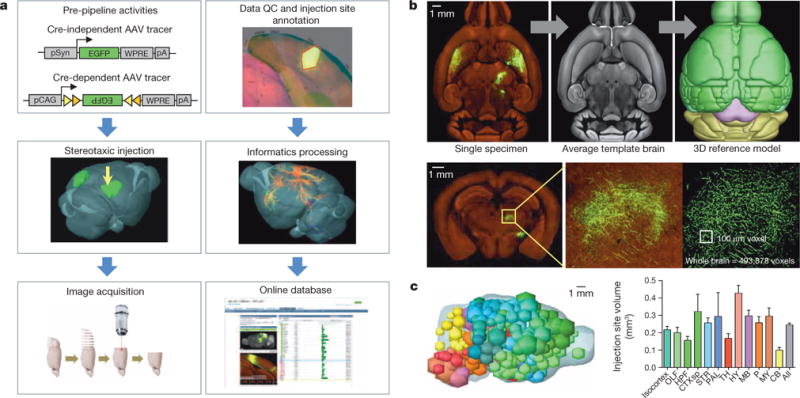
a, The data generation and processing pipeline. QC, quality control. b, The two main steps of informatics data processing: registration of each image series to a 3D template (upper panels) and segmentation of fluorescent signal from background (lower panels). c, Distribution of injection sites across the brain. The volume of the injection was calculated and represented as a sphere. Locations of all these injection spheres are superimposed together (left panel). Mean injection volumes (± s.e.m.) across major brain subdivisions are shown (right panel, see Extended Data Fig. 3).

EGFP-labelled axonal projections were systematically imaged using the TissueCyte 1000 serial two-photon (STP) tomography system²², which couples high-speed two-photon microscopy with automated vibratome sectioning of an entire mouse brain. High x–y resolution (0.35 μm) 2D images in the coronal plane were obtained at a z-sampling interval of 100-μm across the entire brain during a continuous 18.5 h scanning period, resulting in 140 serial sections (a ~750 gigabyte (GB) data set) for each brain (Extended Data Fig. 2a and Supplementary Video 1). Owing to its block-face imaging nature, STP tomography essentially eliminates tissue distortions that occur in conventional section-based histological methods and provides a series of highly conformed, inherently pre-aligned images amenable to precise 3D mapping.

Image series were processed in an informatics pipeline with a series of modules (see Methods). The injection site location of each brain was manually drawn and annotated using the Allen Reference Atlas²³ and other reference data sets when appropriate. Stringent quality control criteria were applied, discarding ~25% of all scanned brains due to insufficient quality in labelling or imaging. Each image set was registered into a 3D Allen Reference Atlas model in two steps (Fig. 1b, upper panels). First, a registration template was created by averaging many image sets, and every image stack was aligned to this average template brain. This process was repeated for multiple rounds, first globally (affine registration) and then locally (deformable registration), each round generating a better average template and more precise alignment of individual brains. The final average template brain, averaged from 1,231 brains, shows remarkably clear anatomical features and boundaries. Second, the average template brain was aligned with the 3D reference model, again using local alignment (Supplementary Video 2).

We developed a signal detection approach and applied it to each section to segment GFP signals from background (Fig. 1b, lower panels). Signals within injection site polygons were computed separately from the rest of the brain. The segmented pixel counts were gridded into 100 × 100 × 100 μm³ voxels to create an isotropic 3D summary of the projection data. These voxels were used for data analysis, real-time data and correlative searches, and visualization of projection relationships in the Brain Explorer.

Meaningful informatics data quantification and comparison relies on the mapping precision of the raw data sets into the 3D reference framework. We investigated registration variability in two ways. First, we selected 10 widely distributed anatomical fiducial points to compare variability among 30 randomly selected brains (Extended Data Fig. 2b). We found a high degree of concordance among individual brains, with median variation < 49 μm in each dimension between each brain and the average template brain, which is comparable to the median inter-rater variation of < 39 μm. The median difference is < 71 μm between each brain and the Reference Atlas. Second, we compared manual and informatics annotations of the injection sites from all Phase I (see below) brains. The informatics-derived assignment of injection site structures had > 75% voxel-level concordance with manual expert annotation for almost all injection sites (Extended Data Fig. 2c). These analyses confirmed the relatively high fidelity of co-registration of raw image data with the Allen Reference Atlas. The remaining difference is mainly due to the imperfect alignment between the average template brain and the Nissl-section-based Reference Atlas (Supplementary Video 2).

Mapping axonal projections in the whole mouse brain

The connectivity mapping was carried out in two phases. In Phase I (regional projection mapping), axonal projections from 295 non-overlapping anatomical regions, defined from the Allen Reference Atlas ontology and tiling the entire brain space (Supplementary Table 1), were characterized in wild-type mice with a pan-neuronal AAV vector expressing EGFP under the human synapsin I promoter (AAV2/1.pSynI.EGFP.WPRE.bGH, Fig. 1a). In Phase II (Cre driver based projection mapping), axonal projections from genetically defined neuronal populations are characterized in Cre driver mouse lines with a Cre-dependent AAV (AAV2/1.pCAG.FLEX.EGFP.WPRE.bGH, Fig. 1a). We only report here on the completed Phase I study, which includes 469 image sets with injection sites covering nearly the entire brain (Fig. 1c, Extended Data Fig. 3 and Supplementary Video 3). Only 18 intended structures were completely missed due to redundancy or injection difficulty (Supplementary Table 1).

We examined multiple projection data sets in detail and found that they were complete in capturing all known projection target sites throughout the brain, sensitive in detecting thin axon fibres, and consistent in quality to allow qualitative and quantitative comparisons. As an example, 7 representative isocortical injections (Fig. 2) reveal distinct projection patterns in the striatum, thalamus, zona incerta, midbrain, pons and medulla. To compare the brain-wide spatial distribution of projections between cortical source regions, we placed each isocortical injection experiment into one of 9 broad functional groups: frontal, motor, anterior cingulate, somatosensory, auditory, retrosplenial, visual, ventral and associational areas (Extended Data Fig. 4). The average percentages of total projection signals into 12 major brain subdivisions showed disproportionately large projections within the isocortex, as well as distinct subcortical distributions.

Figure 2. Whole brain projection patterns from seven representative cortical regions.

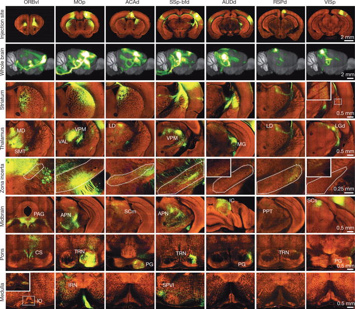
One coronal section at the centre of each injection site is shown in the top row (see Supplementary Table 1 for the full name of each region). In the second row, 3D thumbnails of signal density projected onto a sagittal view of the brain reveal differences in brain-wide projection patterns. The bottom 6 rows show examples of EGFP-labelled axons in representative subcortical regions.

Brain-wide connectivity matrix

After segmentation and registration, we derived quantitative values from segmented signals in each of the ~500,000 voxels contained within each brain. We constructed a brain-wide, inter-areal, weighted connectivity matrix using the entire Phase I experimental data set (Fig. 3, see Supplementary Table 2 for the underlying values). The Allen Reference Atlas contains 863 grey-matter structures at the highest level of the ontology tree (Supplementary Table 1). We focused our analyses on the chosen 295 structures, which are at a mid-ontology level corresponding best with the approximate size of the tracer infection areas (for example, isocortical areas are not subdivided by layers in this matrix), but our techniques may be used at deeper levels in future studies. The projection signal strength between each source and target was defined as the total volume of segmented pixels in the target (summed across all voxels within each target), normalized by the injection site volume (total segmented pixels within the manually drawn injection area).

Figure 3. Adult mouse brain connectivity matrix.

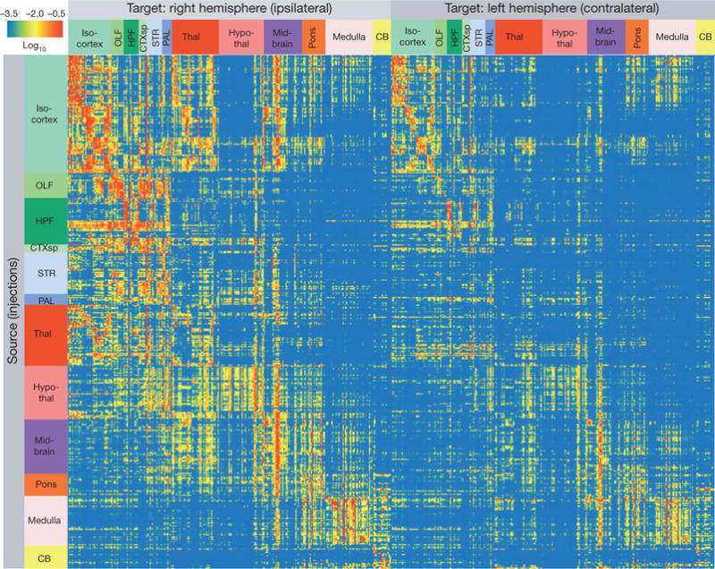
Each row shows the quantitative projection signals from one of the 469 injected brains to each of the 295 non-overlapping target regions (in columns) in the right (ipsilateral) and left (contralateral) hemispheres. Both source and target regions are displayed in ontological order. The colour map indicates log₁₀-transformed projection strength (raw values in Supplementary Table 2). All values less than 10^−3.5 are shown as blue to minimize false positives due to minor tissue and segmentation artefacts and all values greater than 10^−0.5 are shown as red to reduce the dominant effect of projection signals in certain disproportionately large regions (for example, striatum).

The majority of the 469 Phase I image sets are single injections into spatially distinct regions, but a subset of these are repeated injections into the same regions. To assess the consistency of projection patterns across different animals and the reliability of using a single experiment to define connections from any particular region, we compared brain-wide connectivity strengths in 12 sets of duplicate injections (Extended Data Fig. 5). Each pair was highly correlated across a range of projection strengths. Differences between any two points were on average only a half order of magnitude (within one standard deviation). In primate cortex, single tracer injections were also found to reliably predict mean values obtained from repeated injections into the same source²⁴.

The AAV tracer expresses cytoplasmic EGFP, which labels all processes of the infected neuron, including axons and synaptic terminals. Signals associated with the major fibre tracts of the brain, marked in the Allen Reference Atlas, were removed before the informatics quantification. However, there are also areas (for example, striatum) where axons pass through without making synapses. Although passing fibres can generally be distinguished from terminal zones by visual inspection of morphology in the 2D images (axons in terminal zones ramify and contain synaptic boutons, see Extended Data Fig. 6), it is difficult to confidently make this distinction algorithmically. We compared results of terminal labelling using Synaptophysin-EGFP-expressing AAV with the cytoplasmic EGFP AAV (Extended Data Fig. 6). Outside of major fibre tracts, there was high correspondence between synaptic EGFP and cytoplasmic EGFP signals in target regions. Nonetheless, it should be noted that the connectivity matrix contains passing fibre signals within grey matter, the nature of which should be manually examined in 2D section images.

This connectivity matrix (Fig. 3) has several striking features. First, connectivity strengths span a greater than 10⁵-fold range across the brain (Extended Data Fig. 7), suggesting that quantitative descriptions of connectivity must be considered for understanding neural network properties²⁴. Second, there are prevalent bilateral projections to corresponding ipsilateral and contralateral target sites, with ipsilateral projections generally stronger than contralateral ones (total normalized projection volumes from all experiments are 4.3:1 between ipsilateral and contralateral hemispheres). Third, of all possible connections, strong connections are found in only a small fraction. Whereas 63% ipsilateral and 51% contralateral targets have projection strength values above the minimal true positive level of 10⁻⁴ (which has a potential false positive rate of 27%, Extended Data Fig. 7), only 21% ipsilateral and 9% contralateral targets have projection strength values above the intermediate level of 10⁻².

An inter-region connectivity model

Infected neurons in injection sites often span several brain areas. To better describe the mutual connection strengths between ontologically defined regions rather than injection sites, we constructed inter-region connectivity matrices via a computational model (see Supplementary Notes for a detailed description), using segmented projection volumes (Fig. 3) to define connection strengths. Two basic modelling assumptions were used. The first, regional homogeneity, assumes that projections between source X and target Y regions are homogeneously distributed, so that infection of a subarea of the region is representative of the entire region. This allows the value of W_X,Y, a regional connectivity measure, to be inferred from data that can at best only sample the source region. The second assumption, projection additivity, assumes that the projection density of multiple source regions sum linearly to produce projection density in a target region. This allows relative contributions of different sources to be determined for a target region, assuming at least partially independent injections.

The 469 experiments allowed us to compute the mutual connections among 213 regions. The best-fit model (Fig. 4a, see Supplementary Table 3 for the underlying values) results from a bounded optimization followed by a linear regression to determine connection coefficients, assigning statistical confidence (P values) to each connection in the matrix. Based on the bounded optimization, the number of non-zero entries provides an upper bound estimate for sparsity: 36% for the entire brain and 52% for cortico-cortical connections. Using confidence values for each non-zero connection, the lower bound on sparsity is 13% for the entire brain and 32% for cortico-cortical connections.

Figure 4. A computational model of inter-regional connection strengths.

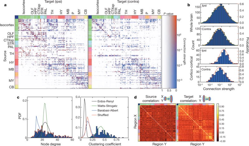
a, The inter-region connectivity matrix, with connection strengths represented in colours and statistical confidence depicted as an overlaid opacity. Note that in this matrix, the sources (rows) are regions, whereas for the matrix of Fig. 3, the sources are injection sites. b, Both whole-brain and cortico-cortical connections can be fit by one-component lognormal distributions (red lines). However, the log distributions of whole-brain connection strengths are best fit by a two-component Gaussian mixture model (green lines). c, Node degree and clustering coefficient distributions for a binarized version of the linear model network, compared against Erdos-Renyi, Watts-Strogatz and Barabasi-Albert networks with matched graph statistics. d, Comparison of the correlation coefficients of normalized connection density between areas, defined as the common source for projections to other regions (left) and as the common target of projections from other regions (right).

Connection strengths spanned ~10⁵-fold range, and negatively correlated with the distance between connected regions (Supplementary Notes and Supplementary Table 4). Based on the Akaike information criterion (AIC), among hypothesized connection strength distributions (lognormal, normal, exponential, inverse Gaussian) the brain-wide data are best fit by a lognormal distribution (Fig. 4b, red lines). However, the log-transformed connection strengths failed to pass the Shapiro-Wilk test for normality (ipsilateral: P = 0.039; contralateral: P = 0.023), and among Gaussian mixture models, a two-component one provided the best fit (Fig. 4b, green lines). For cortico-cortical connections, both intra-and inter-hemispheric distributions are well fit by lognormals (ipsilateral: P = 0.23; contralateral: P = 0.21) individually (Fig. 4b), but they are different enough that when combined the distribution is no longer lognormal (P = 0.0019). This extends previously reported findings that cortico-cortical connections follow a lognormal distribution in the primate^24,25 and mouse cortex²⁶ to the entire mouse brain. These observations combined indicate that connections might be lognormally distributed within a region, yet vary systematically with statistics unique to the region.

Previous studies on connectivity considered global organizational principles from a graph-theory perspective^26–28. We transformed our weighted, directed, connectivity matrix (Fig. 4a) to binary directed and binary undirected data sets. Network analyses (Fig. 4c, see also Supplementary Notes) reveal that the mouse brain has a higher mean clustering coefficient (which gives the ratio of existing over possible connections), 0.42, than expected by a random network^29,30 with identical sparseness, 0.12. Random graphs with matched node degree distribution show a similar drop in clustering coefficient to 0.16. A ‘small-world’ network model³¹ approximates the clustering coefficient distribution after being fit to its mean; however, its node degree distribution poorly matches the data. Here, a better fit is achieved with a scale-free network³²; however, neither model simultaneously fits both distributions.

Next, we analysed similarity in connection patterns between different regions. Similarity is characterized by two measures: correlations between outgoing projections originating in two areas and correlations between incoming projections ending in these two areas. Figure 4d depicts heat maps of correlation coefficients between the same regions of the linear model (Fig. 4a) depicted across the rows (that is, as a common source for other regions), and down the columns (that is, as a common target from other regions). The number of strong correlations is larger than expected by chance, suggesting a tendency of regions to organize into clusters to allow for strong indirect connectivity.

The cortico-striatal-thalamic network

Different cortical areas project to different domains of striatum and thalamus with some degree of topography^33–35. We used 80 isocortical injection experiments to examine this. Spearman’s rank correlation coefficient of segmented projection volumes of all voxels across the entire brain was computed between every pair of experiments, and hierarchical clustering led to 21 distinct groups, each containing 1 to 10 injections (Extended Data Fig. 8a, b). Such grouping effectively divides the cortex into 21 predominantly non-overlapping spatial zones as shown in a flat-map cortex representation (Fig. 5a) defined by similar output projections. To effectively visualize different projection patterns in a common 3D space, voxel densities from 21 selected injections, one (centrally located) from each cluster, were overlaid to create ‘dotograms’ (Fig. 5b, c and Extended Data Fig. 8c), demonstrating that projections from different cortical regions divide up striatum and thalamus into distinct domains.

Figure 5. Topography of cortico-striatal and cortico-thalamic projections.

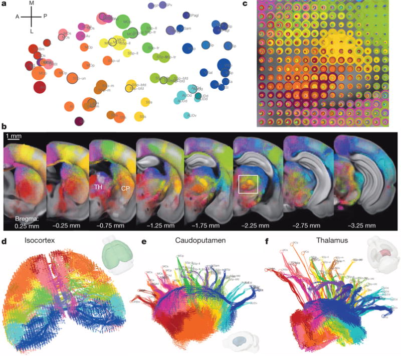
a, Cortical domains in the cortex flat-map. Each circle represents one of 80 cortical injection experiments, whose location is obtained via multidimensional scaling from 3D to allow visualization of all the sites in one 2D plane. The size of the circle is proportional to the injection volume. Clustered groups from Extended Data Fig. 8b are systematically colour-coded. The selected injections for b are marked with a black outline. b, For co-visualization, voxel densities from the 21 selected injections from a are overlaid as ‘dotograms’ at 8 coronal levels for ipsilateral hemisphere. For the dotogram, one circle, whose size is proportional to the projection strength, is drawn for each injection in each voxel; the circles are sorted so that the largest is at the back and the smallest at the front, and are partially offset as a spiral. c, Enlarged view of the dotogram from the area outlined by a white box in b. d, 3D tractography paths in both cortical hemispheres. e, A medial view of 3D tractography paths into the ipsilateral caudoputamen. Voxel starting points are represented as filled circles and injection site end points as open circles. f, A top-down view of 3D tractography paths into the ipsilateral thalamus.

Average inter-group distances (Extended Data Fig. 9a–d) were used to quantify the degree to which inter-group spatial relationships within the cortex are preserved in target domains. Distance matrices for both ipsilateral and contralateral cortical targets were highly correlated with the distance matrix of injection sites, as were ipsilateral striatal and thalamic distance matrices. Weaker correlations were observed in contralateral striatum and thalamus. The computed distance matrices show that the spatial relationship between injection sites is recapitulated in the projections to striatum and thalamus, with some transformation of scale and rotation.

This highly synchronized topography can be determined via virtual tractography. Real tractography (following single axons) cannot be done because of the discrete 100-μm sampling between sections. Instead, from every voxel we computed a path back to the injection site by finding the shortest density-weighted distance through the voxels. The 3D tractography paths were plotted for both cortical hemispheres (Fig. 5d and Extended Data Fig. 9e), ipsilateral striatum and thalamus (Fig. 5e, f). The tractography shows that the paths themselves also retain the same spatial organization. In particular for the thalamus, anterior groups pass through fibre tracts in the striatum, narrowing through the globus pallidus, before spreading throughout the thalamus (Extended Data Fig. 9f). Posterior groups (RSP, VIS) bypass the striatum but retain a strict topography following the medial/lateral axis (Fig. 5f).

Although the striatum is a cellularly homogeneous structure that can be subdivided into distinct domains selectively targeted by cortical and other inputs³⁶ (Fig. 5e), the thalamus is highly heterogeneous, composed of up to 50 discrete nuclei³⁷, receiving and relaying diverse sensory, motor, behavioural state and cognitive information in parallel pathways to and from the isocortex. We constructed a comprehensive wiring diagram between major, functionally distinct cortical regions and thalamic nuclei in the ipsilateral hemisphere (Fig. 6 and Extended Data Fig. 10), by combining the quantitative connectivity matrix (Fig. 3) with the linear model (Fig. 4a), manual proof-checking in the raw image sets, and cross-referencing published literature (83 publications, mostly from rat data, see Extended Data Fig. 10). This wiring diagram demonstrates specific point-to-point interconnections between corresponding clusters that divide the cortico-thalamic system into six functional pathways: visual, somatosensory, auditory, motor, limbic and prefrontal. We also observed cross-talk between these pathways, mediated by specific associational cortical areas and integrative thalamic nuclei.

Figure 6. A wiring diagram of connections between major cortical regions and thalamic nuclei.

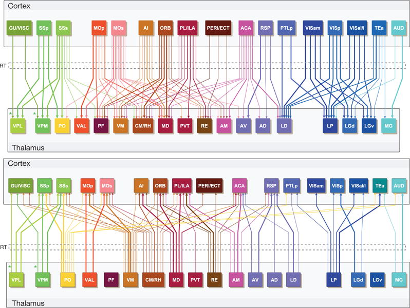
Upper and lower panels show projections from cortex to thalamus or from thalamus to cortex, respectively (ipsilateral projections only). Colour coding of different cortical regions and their corresponding thalamic nuclei is similar to the flat-map cortex in Fig. 5a. Thickness of the arrows indicates projection strength, which is shown in three levels as in Extended Data Fig. 10 and corresponds roughly to the red, orange and yellow colours in the raw connectivity matrix (Fig. 3). LGv and PF do not have significant projections to cortex. The reticular nucleus of the thalamus (RT) (the dashed box) is placed in between cortex and thalamus to illustrate its special role as a relay nucleus which all cortico-thalamic and thalamo-cortical projections pass through and make collateral projections into. The asterisks indicate that cortico-thalamic and thalamo-cortical projections in the gustatory/visceral pathway are between GU/VISC cortical areas and VPMpc/VPLpc nuclei (instead of VPM/VPL). See Supplementary Table 1 for the full name of each region.

The specific observations from our data are mostly consistent (with a few additions) with extensive previous studies in rats and the fewer number of studies in mice (Extended Data Fig. 10) as well as with studies in other mammalian species^37–39, providing a comprehensive and unifying view of mouse cortico-thalamic connections for the first time. Much work is still needed to obtain a full picture of connectivity in the cortico-thalamic system, including intra-cortical and intra-thalamic connections, their relationships with the interconnections between cortex and thalamus, and the exquisite cortical laminar specificity of the originating and terminating zones of many of these connections^5,38,40.

Discussion

The standardized projection data set and the informatics framework built around it provide a brain-wide, detailed and quantitative connectivity map that is the most comprehensive, to date, in any vertebrate species. The high-throughput whole-brain mapping approach is remarkably consistent across animals, with an average correlation of 0.90 across 12 duplicate sets of mice (Extended Data Fig. 5). Informatics processing of the data set, such as co-registration and voxelization, helps with direct comparison between any image series, and systematic modelling and computational analyses of the entire network. Furthermore, the entire data set preserves the 3D spatial relationship of different domains, pathways and topography (Fig. 5). Thus, our connectivity atlas lays the groundwork for large-scale analyses of global neural networks, as well as networks within and between different neural systems.

As an initial analysis of this large-scale data set, we present an examination of both general principles of whole brain architecture and specific properties of cortical connections. We found that projections within the ipsilateral hemisphere and to the corresponding locations in the contralateral hemisphere are remarkably similar across the brain (Figs 3 and 4; Pearson’s r = 0.595), with the contralateral connection strengths significantly weaker than ipsilateral ones. The mouse brain shows defining features of both small-world and scale-free networks, that is, it clusters and has hubs; but neither of these models in isolation can fully explain it. Interestingly, the connection strengths at both cortico-cortical and whole-brain levels show lognormal distributions, that is, long-tailed distributions with small numbers of strong connections and large numbers of weak connections. In connections among isocortex, striatum and thalamus, clustering analysis and virtual tractography recapitulate anatomical parcellation and topography of functional domains and projection pathways (Fig. 5). The extensive reciprocal connections between isocortex and thalamus (Fig. 6) further illustrate general principles of network segregation and integration.

Our Connectivity Atlas represents a first systematic step towards the full understanding of the complex connectivity in the mammalian brain. Through the process, limitations of the current approach and opportunities for future improvement can be identified. On the technical side, any potential new connections identified in the Phase I data set (which does not yet have extensive redundancy in regional coverage) will need to be confirmed with more data. Also, we cannot exclude the possibility that the AAV tracer we chose to use (with the specific promoter and serotype) may not be completely unbiased in labelling all neuronal types. The connectivity matrix has been shown to contain false positive signals (Extended Data Fig. 7), mainly due to tissue and imaging artefacts and injection tract contaminations. The connectivity matrix based on cytoplasmic EGFP labelling does not distinguish passing fibres from terminal zones, and examination of raw images is needed to help with such distinction, using features such as ramification of axon fibres, and boutons or enlargements in axons. The Atlas could also be enhanced in the future with more systematic mapping using synaptic-terminal-specific viral tracers as shown (Extended Data Fig. 6). Regarding signal quantification, we chose to use projection volume (sum of segmented pixel counts) over projection fluorescence intensity (sum of segmented pixel intensity), because we found the former more reliable and less variable across different brains (even after normalization). However, the use of projection volume will probably underestimate the strength of dense projections. Thus, the true range of projection strengths may go beyond the 10⁵-fold reported here. Finally, we observed that the alignment between the average template brain and our existing Reference Atlas model (which was drawn upon Nissl sections) is not perfect, which leads to a degree of registration imprecision that could affect the accuracy of the quantitative connectivity matrices. Our work shows the need to generate a new reference model based on a realistic 3D brain, such as the average template brain presented here. Our data set can also help this by adding connectivity information to improve anatomical delineations previously defined solely by cyto- and chemoarchitecture.

Beyond the above technical issues, identities of the postsynaptic neurons at the receiving end of the mapped connections are not labelled and therefore unknown. Microscale, synaptic-level details are missing, and electrical connections through gap junctions are not revealed. Moreover, our mesoscale connectome provides a static, structural connectivity map, which is necessary but insufficient for understanding function. Moving from here to functional connectivity and circuit dynamics in a living brain will require fundamentally different approaches⁴¹. One important aspect concerns the types of synapses present in each connectional path, as determined by their neurotransmitter contents and their physiological properties. Anatomical connection strength (for example, numbers of axon fibres and boutons) needs to be combined with physiological connection properties (for example, excitatory vs inhibitory types of synapses, fast vs slow neuro transmission, and the specific strength and plasticity of each synapse) to yield a true functional connection strength.

With the goal of bridging structural connectivity and circuit function⁴¹, we have taken a genetic approach, using AAV viral tracers that express EGFP in either a pan-neuronal or cell-type-specific manner. The same neural networks mapped here can be further investigated by similar viral vectors expressing tools for activity monitoring (for example, genetically encoded calcium indicators) and activity manipulation (for example, channelrhodopsins)¹⁶. Furthermore, our ongoing efforts of Cre-driver dependent tracing will allow more specific connectivity mapping from discrete areas and specific functional cell types. Such cell-type-specific connectivity mapping is perhaps the greatest advantage of the genetic tracing approach, allowing dissection of differential projection patterns from different neuronal types that are often intermingled in the same region. The genetic tracing approach can be further extended into identification of inter-connected pre- and postsynaptic cell types and individual cells, using approaches such as retrograde or anterograde trans-synaptic tracing^42–44. Our approach can also be applied to animal models of human brain diseases and the connectivity data generated here can be instructive to human connectome studies, which will help to further our understanding of human brain connectivity and its involvement in brain disorders.

METHODS SUMMARY

C57BL/6J male mice at age P56 were injected with EGFP-expressing AAV using iontophoresis by the stereotaxic method. The brains were scanned using the STP tomography systems. Images were subject to data quality control and all the injection sites were manually annotated. All the image sets were co-registered into the 3D reference space. EGFP-positive signals were segmented from background, and binned at voxel levels for quantitative analyses. The raw connectivity data are served with various navigation tools on the web through the Allen Institute’s data portal. See the full Methods section for detailed descriptions.

METHODS

All experimental procedures related to the use of mice were approved by the Institutional Animal Care and Use Committee of the Allen Institute for Brain Science, in accordance with NIH guidelines.

Outline of the Connectivity Atlas data generation and processing pipeline

A standardized data generation and processing platform was established (Fig. 1a). Viral tracers were validated and experimental conditions were established through pre-pipeline activities. C57BL/6J mice at age P56 were injected with viral tracers using iontophoresis by the stereotaxic method. Six STP tomography systems generated high-resolution images from up to 6 brains per day. Images were subject to data quality control and all the injection sites annotated. A stack of qualified 2D images then underwent a series of informatics processes. The image data and informatics products as well as all metadata are stored, retrieved and maintained using our laboratory information management system (LIMS). The generated connectivity data are served with various navigation tools on the web through the Allen Institute’s data portal along with other supporting data sets.

Stereotaxic injections of AAV using iontophoresis

Recombinant adeno-associated virus (AAV) expressing EGFP was chosen as the anterograde tracer to map axonal projections because of several advantages over conventional neuroanatomical tracers¹⁹. First, AAV mediates robust fluorescent labelling of the soma and processes of infected neurons, which can be coupled with direct imaging methods for high-throughput production without additional histochemical staining steps. Second, compared to conventional tracers which often have mixed anterograde and retrograde transport, retrograde labelling with AAV (except for certain serotypes) is generally negligible. In this study, retrogradely infected cells were seen only rarely. Notable exceptions are found in specific circuits that might have certain types of strong presynaptic inputs, such as the entorhinal cortex projection to hippocampal subregions dentate gyrus and CA1, where retrogradely infected input cells can be brightly labelled. Finally, perhaps the greatest advantage of using AAV over conventional tracers is the flexible molecular strategies that can be used to introduce various transgenes and to label specific neuronal populations by combining cell-type-selective Cre driver mice with AAV vectors harbouring a Cre-dependent expression cassette.

To optimize the tracing approach for the large-scale atlas data generation, we tested various AAV constructs, serotypes and injection methods. We selected AAV vectors that express EGFP at the highest levels. We found that AAV serotype 1 produces the most robust and uniform neuronal tropism and that iontophoretic delivery of AAV gives rise to the most consistent and confined viral infection volume. Thus, the entire atlas data generation was standardized with the use of AAV serotype 1 and iontophoresis for stereotaxic injections²⁰.

Stereotaxic coordinates were chosen for each target area based on The Mouse Brain in Stereotaxic Coordinates⁴⁵. For the majority of target sites, the anterior/posterior (AP) coordinates are referenced from Bregma, the medial/lateral (ML) coordinates are distance from midline at Bregma, and the dorsal/ventral (DV) coordinates are measured from the pial surface of the brain. For several of the most caudal medullary nuclei (for example, gracile nucleus and spinal nucleus of the trigeminal, caudal part), the calamus (at the floor of the fourth ventricle) is used as a registration point instead of Bregma. For many cortical areas, injections were made at two depths to label neurons throughout all six cortical layers and/or at an angle to infect neurons along the same cortical column. For laterally located cortical areas (for example, orbital area, medial part; prelimbic area; agranular insular area), the injections were made at two adjacent ML coordinates for the same reason, since the pipette angle required for injection along the cortical column is nearly 90°, beyond our technical limit. The stereotaxic coordinates used for generating data are listed under the Documentation tab in the data portal.

Adult male C57BL/6J mice (stock no. 00064, The Jackson Laboratory, Bar Harbour, ME) were used for AAV tracer (AAV2/1.pSynI.EGFP.WPRE.bGH, Penn Vector Core, Philadelphia, PA) injections at P56 ± 2 postnatal days. Mice were anaesthetized with 5% isoflurane and placed into a stereotaxic frame (modelno. 1900, David Kopf Instruments, Tujunga, CA). For all injections using Bregma as a registration point, an incision was made to expose the skull and Bregma and Lambda landmarks were visualized using a stereomicroscope. A hole overlying the targeted area was made by first thinning the skull using a fine drill burr until only a thin layer of bone remained. A microprobe and fine forceps were used to peel away this final layer of bone to reveal the brain surface. For targeting caudal nuclei in the medulla, ketamine-anaesthetized mice were placed in the stereotaxic frame with the nose pointed downward at a 45–60 degree angle. An incision was made in the skin at the base of the skull and muscles were bluntly dissected to reveal the posterior atlanto-occipital membrane overlying the surface of the medulla. A needle was used to puncture the membrane and the calamus was visualized.

All mice received one unilateral injection into a single target region in the right hemisphere. Glass pipettes had inner tip diameters of 10–20 μm. The majority of injections were done using iontophoresis with 3 μA at 7 s ‘on’ and 7 s ‘off’ cycles for 5 min total. These settings resulted in infection areas of approximately 400–1,000 μm in diameter, depending on target region. Reducing the current strength to 1 mA decreased the area of infected neurons, and was used when 3 μA currents produced infection areas larger than ~700 μm. Mice quickly recovered after surgery and survived for 21 days before euthanasia. Injection sites ranged from 0.002 to 1.359 mm³ in volume, with an average size of 0.24 mm³ across all 469 data sets.

Serial two-photon tomography

Mice were perfused with 4% paraformaldehyde (PFA). Brains were dissected and post-fixed in 4% PFA at room temperature for 3–6 h and then overnight at 4 °C. Brains were then rinsed briefly with PBS and stored in PBS with 0.1% sodium azide before proceeding to the next step. Agarose was used to embed the brain in a semisolid matrix for serial imaging. After removing residual moisture on the surface with a Kimwipe, the brain was placed in a 4.5% oxidized agarose solution made by stirring 10 mM NaIO₄ in agarose, transferred through phosphate buffer and embedded in a grid-lined embedding mould to standardize its placement in an aligned coordinate space. The agarose block was then left at room temperature for 20 min to allow solidification. Covalent interactions between brain tissue and agarose were promoted by placing the solidified block in 0.5% sodium borohydride in 0.5 M sodium borate buffer (pH 9.0) overnight at 4 °C. The agarose block was then mounted on a 1 × 3 glass slide using Loctite 404 glue and prepared immediately for serial imaging.

Image acquisition was accomplished through serial two-photon (STP) tomography²² using six TissueCyte 1000 systems (TissueVision, Cambridge, MA) coupled with Mai Tai HP DeepSee lasers (Spectra Physics, Santa Clara, CA). The mounted specimen was fixed through a magnet to the metal plate in the centre of the cutting bath filled with degassed, room-temperature PBS with 0.1% sodium azide. A new blade was used for each brain on the vibratome and aligned to be parallel to the leading edge of the specimen block. Brains were imaged from the caudal end. We optimized the imaging conditions for both high-throughput data acquisition and detection of single axon fibres throughout the brain with high resolution and maximal sensitivity. The specimen was illuminated with 925 nm wavelength light through a Zeiss ×20 water immersion objective (NA = 1.0), with 250 mW light power at objective. The two-photon images for red, green and blue channels were taken at 75 μm below the cutting surface. This depth was found optimal as it is deep enough to avoid any major groove on the cutting surface caused by vibratome sectioning but shallow enough to retain sufficient photons for high contrast images. In order to scan a full tissue section, individual tile images were acquired, and the entire stage was moved between each tile. After an entire section was imaged, the x and y stages moved the specimen to the vibratome, which cut a 100-μm section, and returned the specimen to the objective for imaging of the next plane. The blade vibrated at 60 Hz and the stage moved towards the blade at 0.5 mm per sec during cutting. Images from 140 sections were collected to cover the full range of mouse brain. It takes about 18.5 h to image a brain at an x,y resolution of ~0.35 μm per pixel, amounting to ~750 GB worth of images per brain. Upon completion of imaging, sections were retrieved from the cutting bath and stored in PBS with 0.1% sodium azide at 4 °C.

Image data processing

The informatics data pipeline (IDP)⁴⁶ manages the processing and organization of the image and quantified data for analysis and display in the web application. The two key algorithms are signal detection and image registration.

The signal detection algorithm was applied to each image to segment positive fluorescent signals from background. Image intensity was first rescaled by square root transform to remove second-order effects followed by histogram matching at the midpoint to a template profile. Median filtering and large kernel low pass filter was then applied to remove noise. Signal detection on the processed image was based on a combination of adaptive edge/line detection and morphological processing. High-threshold edge information was combined with spatial distance-conditioned low-threshold edge results to form candidate signal object sets. The candidate objects were then filtered based on their morphological attributes such as length and area using connected component labelling. In addition, high intensity pixels near the detected objects were included into the signal pixel set. In a post-segmentation step, detected objects near hyper-intense artefacts occurring in multiple channels were removed. It should be noted that passing fibres and terminals are not distinguished. The output is a full resolution mask that classifies each 0.35 μm × 0.35 μm pixel as either signal or background. Isotropic 3D summary of each brain is constructed by dividing each image into 100 μm × 100 μm grid voxels. Total signal is computed for each voxel by summing the number of signal-positive pixels in that voxel.

The highly aligned nature from section to section throughout a single brain allowed us to simply stack the section images together to form a coherent reconstructed 3D volume. Each image stack was then registered to the 3D Allen Reference Atlas model. To avoid possible bias introduced by using a single specimen as template and to increase the convergence rate of the registration algorithm, a registration template was created by iteratively averaging 1,231 registered and resliced brain specimens. A global affine (linear) registration to the template was first performed using a combination of image moments and maximizing normalized mutual information between the red channel of the image stack and the template using a multi-resolution gradient descent optimization. A B-spline based deformable registration was then applied using a coarse-to-fine strategy through four resolution levels with decreasing smoothness constraints. In each generation, a new template was created using the previous generation results to further improve registration convergence. The template was then deformably registered to the 3D reference model by maximizing the mutual information of large structure annotation and the template intensity.

Segmentation and registration results are combined to quantify signal for each 100 μm × 100 μm × 100 μm voxel in the reference space and for each structure in the ontology by combining voxels from the same structure in the 3D reference model. To generate the raw connectivity matrix (Fig. 3), the projection signal was quantified by summing the number of segmented pixels in every voxel, and scaling this value to a mm³ volume. The voxel values within each of the 469 injection sites (source) or each of the 295 target sites in either hemisphere were binned and summed based on which structure the voxel belongs to. The target structure values presented across the columns are normalized by each experiment’s injection volume to allow comparison between injections. Fluorescent signals within each injection area were excluded from projection signal calculation.

The informatics data processing supports key features in the web application, including an interactive projection summary graph for each specimen, an image synchronization feature to browse images from multiple injections, reference atlases and other data set in a coordinated way, and on-the-fly search services to search for a specimen with specific projection profiles. Further details of the pipeline processing and web application features are described under the documentation tab in the data portal.

Quality control, injection site annotation and polygon drawing

A rigorous manual quality control protocol was established which includes identification of the injection structure(s) according to the Allen Reference Atlas ontology, delineation of the injection site location and decisions on failing an experiment due to production issues affecting specimen and image quality. Severe artefacts such as missing tissue or sections, poor orientation, edge cutoff, tessellation and low signal strength lead to elimination of the entire image series. In some cases, the quality control process extended to identification and masking of areas of high intensity/high frequency artefacts and areas of signal dropout. This information is used in downstream search and analysis to reduce false positive and false negative returns.

For each passed image series, the anatomical location(s) of injection site was annotated based on the Allen Reference Atlas²³ and The Mouse Brain in Stereotaxic Coordinates⁴⁵. If an injection has hit multiple structures, the structure containing the majority of the tracer is named as the primary injection structure, and any other structures containing tracer-infected neurons are considered secondary injection structures. Polygons were manually drawn overlaying the cell bodies of infected neurons for each passed injection with an electronic region of interest for ease of injection site location by the end user, and further informatics processing. After data registration into the 3D reference space, injection sites were also annotated computationally. In most cases, results obtained from manual and informatics annotations are the same. The manually derived primary and secondary injection structures are provided as search entries for the Atlas, while the computationally derived sites are available on the projection summary page for each experiment.

Extended Data

Extended Data Figure 1. AAV/BDA tracer comparison, using a primary motor cortex (MOp) injection as an example.

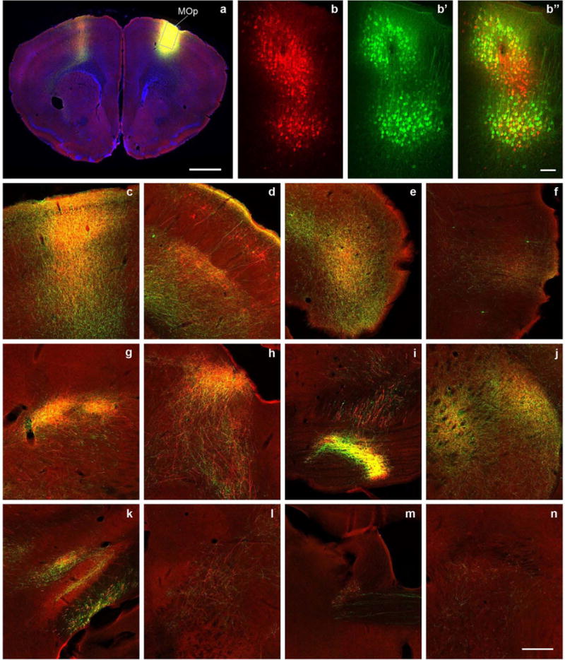
The cortical and subcortical projections from MOp injection are labelled similarly with the AAV tracer (green) and conventional tracer BDA (red). a, Injection sites of AAV and BDA are mostly overlapping (yellow), with a blue DAPI counterstain. b, Confocal image taken from the box in a shows BDA tracer uptake in individual neurons at the injection site. b’, The same box in a shows AAV infection of individual neurons. b”, Overlay of b and b’ shows the presence of both tracers in the same region and their colocalization in some neurons (yellow). c–f, Examples of cortical projections in the contralateral primary motor cortex, ipsilateral primary somatosensory cortex, agranular insular area (dorsal part), and perirhinal cortex labelled with red, green, or yellow. g–n, Examples of subcortical projections in the ipsilateral ventral posterolateral nucleus of the thalamus and posterior nucleus of the thalamus, superior colliculus, pontine grey, caudate putamen, zona incerta and subthalamic nucleus, midbrain reticular nucleus, parabrachial nucleus, and contralateral bed nucleus of the anterior commissure. Scale bars are 1,000 μm (a); 100 μm in (b, b’ and b”); and 258 μm (c–n). Approximately 18 brain regions were selected throughout the brain to represent broad anatomical areas and diverse cell types (3 cortical and 15 subcortical structures). AAV and BDA were co-injected into each selected brain region in wild-type mice using a sequential injection method developed to target virtually the same anatomical region. For most cases, the anatomical area(s) of tracer uptake are well matched. We found the long-range projections from all studied regions with both tracers. Their patterns were similar between the two tracers in mostly overlapped injection cases. There were more retrogradely labelled neurons with BDA than AAV, although a few retrograde neurons were observed in all studied regions with both tracers. BDA was clearly uptaken by passing fibres in some injections but AAV was not.

Extended Data Figure 2. Consistency among individual STP tomography image sets.

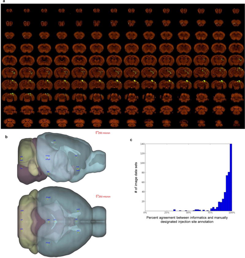
a, High-resolution images of 140 serial sections of a single brain are shown as an example (injection into the primary visual area). The injection site and major projection targets can be easily observed in this ‘contact-sheet’ view. b, Registration variability study. A set of ten 3D fiducial points of interest (POIs) were manually identified on the Nissl 3D reference space, the average template brain, and in 30 randomly selected individual image sets by three raters independently. The POIs were selected such that they span the brain and can be easily and repeatedly identified in 3D. Each POI (p) from each experiment was then projected into 3D reference space (p’) using the transform parameters computed by the Alignment module. Statistics were gathered on the target registration error between p’ and its ‘gold standard’ correspondence (computed as the mean of the labelling of 3 raters) in the Nissl (pNissl) and template (ptemplate) volumes. In summary, for all POIs in template space, the observed median variation in each direction are 28 μm for left-right, 35 μm for inferior-superior, and 49 μm for anterior-posterior. In Nissl space, these observed median variations are 42, 71 and 60 μm, respectively. The registration variations in different directions are shown here. For each POI, the green dot shows the position in template space (ptemplate) and the red dot shows the position in Nissl space (pNissl). The small yellow bar shows the median variation (among 30 image sets) away from ptemplate in each direction. POIs: AP: area postrema, midline; MM: medial mammillary nucleus, midline; cc1: corpus callosum, midline; cc2: corpus callosum, midline; acoL, acoR: anterior commisure, olfactory limb; arbL, arbR: arbor vitae; DGsgL, DGsgR: dentate gyrus, granule cell layer. c, Percent agreement between computationally assigned injection site voxels and manually assigned injection structures. Each histogram data point corresponds to a single injection, and 100% indicates that every injection site voxel was computationally assigned to a structure included on the manually annotated injection structures list. Voxels which were computationally assigned to fibre tracts or ventricles are excluded from the computation. Neither fibre tracts nor ventricles were incorporated into the manual annotation process; their exclusion allows for a more commensurate comparison.

Extended Data Figure 3. Distribution of injection sites across the brain.

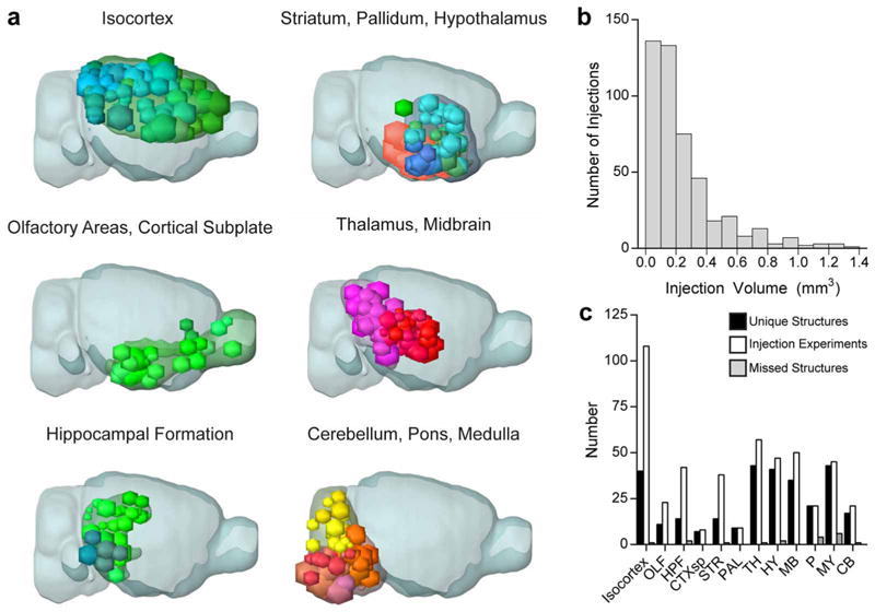
a, Locations of injection spheres within 12 major brain subdivisions are shown as a projection onto the mouse brain in sagittal views. n = 108 isocortex, 23 olfactory areas (OLF), 42 hippocampal formation (HPF), 8 cortical subplate (CTXsp), 38 striatum (STR), 9 pallidum (PAL), 57 thalamus (TH), 47 hypothalamus (HY), 50 midbrain (MB), 21 pons (P), 45 medulla (MY) and 21 cerebellum (CB). b, Frequency histogram for the injection site volumes of all 469 data sets is shown. c, The Allen Reference Ontology was collapsed into 295 non-overlapping, unique, anatomical structures for analyses, distributed across major brain subdivisions as shown (black bars). For most structures, a single injection was sufficient to infect the majority of neurons in that region. For larger structures (for example, primary motor cortex), multiple injections were made into several, spatially separate locations. The majority of these 295 regions have at least one injection targeted to that structure as either the primary or secondary injection site (white bars); only 18 structures are not covered at all (grey bars, for details see Supplementary Table 1). These missed structures (minimal to no infected cells in either the primary or secondary injection sites) were either very small (for example, nucleus y in the medulla), purposefully left out due to the presence of other injections under the same large parent structure (for example, four of the cerebellar cortex lobules), or technically challenging to reach via stereotaxic injection (for example, suprachiasmatic nucleus).

Extended Data Figure 4. Distribution of whole brain projections from different cortical source areas.

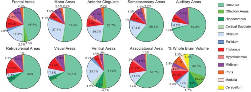
Pie charts show the percentage of total projection volume across all voxels outside of the injection site distributed in the 12 major brain subdivisions from both hemispheres. Each pie chart represents the average of 4 to 27 cortical injections grouped by the broad regions listed. A pie chart key of the volume distribution (number of voxels per structure/total number of voxels per brain) of these 12 subdivisions is at the bottom right for comparison. The largest projection signal from each cortical injection is found within isocortex (range of 45.4–69.8% of projection signals depending on source region, with an average of 59% for all cortical injections), although the isocortex accounts for only 30.2% of total brain volume. Differences in the subcortical distribution of relative signal strength between cortical sources were also observed. For example, within the striatum (light blue), the percentage of total signal is low from auditory, retrosplenial and visual areas (6.2%, 3.4% and 7.6%, respectively), but much greater from frontal, motor, cingulate and somatosensory areas (16.5%, 27.7%, 20.3% and 17.6%, respectively).

Extended Data Figure 5. Variability of brain-wide projection signal strength.

To examine animal-to-animal variability in projection patterns, 12 sources with two spatially overlapping injection experiments were identified from the full data set of tracer injections shown in Fig. 3. a, Rows show segmented projection volumes normalized to the injection volume (log₁₀-transformed) in the 295 ipsilateral target regions for each of 2 individual overlapping tracer injections per source region indicated (above and below solid black line). The colour map is as shown in Fig. 3. b, Maximal density projections of whole brain signals from each of the two spatially overlapping injection experiments per source region visibly demonstrate consistency of brain-wide connections. Scatter plots of all ipsilateral and contralateral target structure values above a minimum threshold in both members of the pair (log₁₀ = −3.5; non-blue values from a) show significant correlations between each pair of injections across a four orders of magnitude range of projection strengths. Values in the scatter plots are Pearson’s correlation coefficients (r). Note that in some cases (for example, PTLp) axon pathways appear to be labelled in only one of the pair. This could be due to random differences in the proportion of corticospinal projecting neurons labelled in a particular injection within the same source area. Signal in large annotated white matter tracts are computationally removed from the connectivity matrix, and thus not included in the scatter plots. c, Detected fluorescent signals from each of two injections into the same location of primary somatosensory cortex registered and overlaid with the average template brain (grey). Lower 2 rows, 2D raw images from each injection experiment at different anterior-posterior levels. The centres of these injection sites are in the far left panel and their major targets are in the right panels. See Supplementary Table 1 for the corresponding full name and acronym for each region.

Extended Data Figure 6. Cytoplasmic EGFP and synaptophysin-EGFP AAV tracer comparison, using primary motor cortex (MOp) injections as an example.

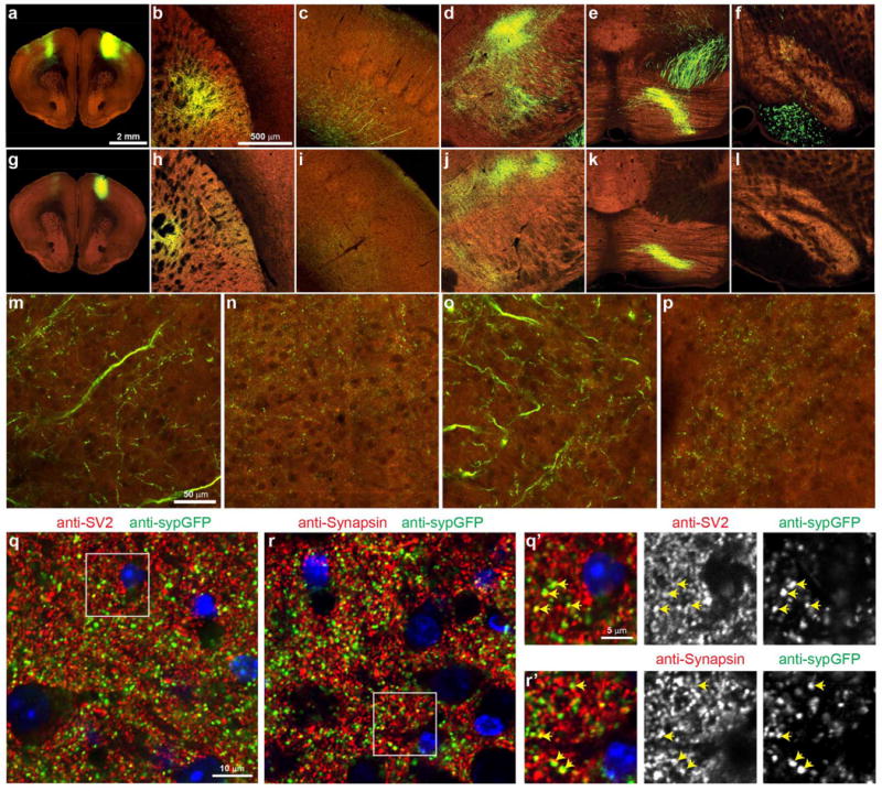
a–f, Two-photon images showing an example of the labelling obtained using the Phase I virus for whole-brain projection mapping, which consists of a human Synapsin I promoter driving expression of EGFP. g–l, To compare cytoplasmic labelling of projections and identification of terminal regions with a presynaptic reporter virus, we made a construct with the same hSynapsin promoter driving expression of a triple reporter cassette (AAV2/1.pSynI.nls-hrGFP-T2A-tagRFP-T2A-sypGFP.WPRE.bGH): a nuclear localization signal attached to humanized Renilla GFP (nls-hrGFP), a T2A sequence followed by cytoplasmic tagRFP, a second T2A sequence, and the synaptophysin-EGFP fusion (sypGFP). Owing to the two-photon imaging wavelength used (925 nm), the tagRFP (red) signal is weak to non-existent in these images. a, g, An image at the centre of the infected area after injection into the same region of MOp with the Phase I cytoplasmic viral tracer (a) and the nuclear and synaptic reporter viral tracer (g). Examples of viral labelling in the caudoputamen (b, h), somatosensory cortex (c, i), thalamus (d, j), pontine grey (e, k) and inferior olivary complex in the medulla (f, l) are shown for both tracers. The cytoplasmic viral tracer labels axons, revealing dense branching patterns in presumed terminal zones. The presynaptic reporter virus predominantly shows a punctate pattern of labelling consistent with presynaptic protein expression patterns, and indicative of terminal zones. Punctate or diffuse labelling was observed with the synaptic reporter virus in nearly all MOp target regions manually and computationally identified using the cytoplasmic reporter, including those with both large and small signals. Fluorescent signal originating in fibres outside of large white matter tracts are included in the signal quantification and matrix shown in Fig. 3, but signals from these large annotated fibre tracts are computationally removed. m–p, High-resolution images of terminal zones in the somatosensory cortex (m) and thalamus (o) identified using the cytoplasmic viral tracer show axon ramification and punctate structures consistent with bouton labelling, similar to the synaptic reporter in the corresponding regions (n, p). q–r’, To validate the presynaptic expression of the sypGFP fusion protein, sections including and adjacent to the thalamic region shown in j were collected after two-photon imaging and immunostained with antibodies against GFP (chicken polyclonal 1:500, Aves Labs, Inc. #GFP-1020) and synapsin I (rabbit polyclonal, 1:200, Millipore, #AB1543P) or GFP (rabbit polyclonal, Life Technologies, #A-11122) and SV2 (mouse monoclonal, DSHB, SV2-supernatant) presynaptic proteins. q, r, Confocal images at a single plane show punctate labelling indicative of presynaptic boutons for both sypGFP and synapsin or SV2. Many puncta were colocalized (yellow arrows show select examples in q’ and r’), although quantification was not reliable due to the very high density of presynaptic labelling by anti-Synapsin and anti-SV2.

Extended Data Figure 7. Distribution of log₁₀-transformed normalized projection volumes from the entire matrix presented in Fig. 3.

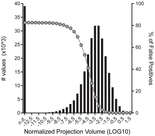
The values (left-hand y axis, black bars) were number of target regions and derived from Supplementary Table 2. The entire range of the normalized projection volumes in this matrix was between log₁₀ = −14 and log₁₀ = 1.5, and it peaked between log₁₀ = −3.5 and log₁₀ = −3.0. A manual analysis of true positive and true negative signals from 20 randomly chosen injection experiments, representing the range of injection sizes, was used to estimate the false positive rate at different threshold levels, shown on the right-hand y axis (grey circles). True positive values predominantly fall within the range of log₁₀ = −4 to 1.5. For example, at a threshold of log₁₀ = −4, the false positive rate was 27%, dropping to 14.5% at log₁₀ = −3.5. False positives were almost exclusively due to small segmentation artefacts in areas without actual fluorescently labelled axon fibres.

Extended Data Figure 8. Cortical domains identified by clustering analysis of projection patterns.

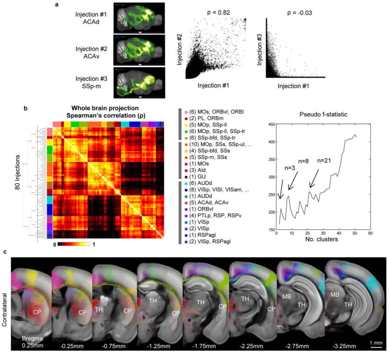
Eighty injections were used in the analysis for which the injection site is strictly within the isocortex and injection volume >0.07 mm³. a, Scatter plot of the voxel densities (excluding injection sites) of the whole brains from two nearby anterior cingulate injections (ACAd and ACAv) shows a strong correlation between the two (Spearman’s ρ = 0.82), whereas that of two distant injections (ACAd and SSp-m) shows little correlation (ρ = −0.03). b, Hierarchical clustering of the projection pattern based on Spearman’s rank correlation coefficient of voxel density over the entire brain. The pseudo-F statistics measures the coherence of clusters and is the ratio of mean sum of squares between groups to the mean sum of squares within group. Peaks in the pseudo-F statistics (for example, at n = 3, 8 and 21 clusters) are indicators of greater cluster separation. For n = 21 clusters, a systematic colour-code is given to each cluster to provide a visual guide to their cortical location (Fig. 5a), the numbers in parentheses indicate the number of injections in each group. c, Voxel densities from the 21 selected injections from Fig. 5a are overlaid as ‘dotograms’ at 8 coronal levels for the contralateral hemisphere.

Extended Data Figure 9. Topography of cortico-striatal and cortico-thalamic projections.

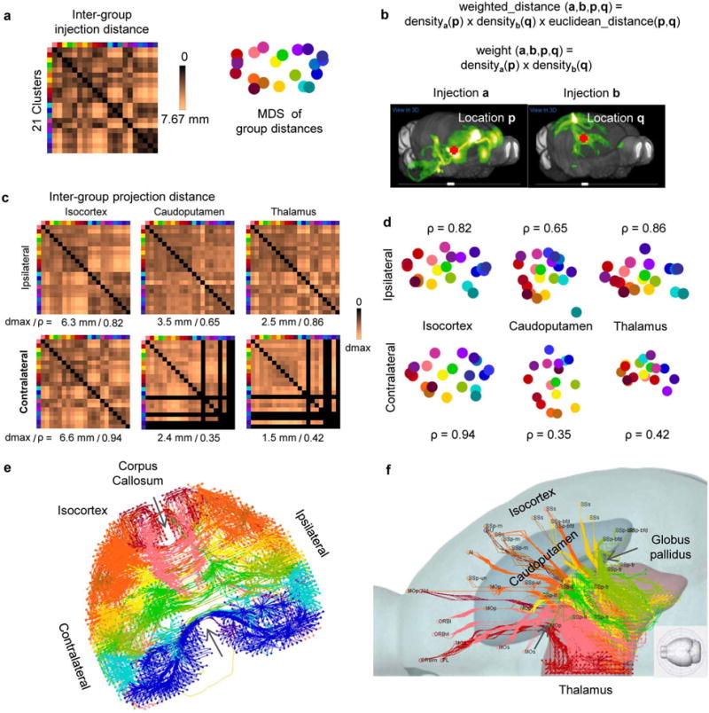
Average inter-group distance was used to quantify the degree of which inter-group spatial relationship within the cortex is preserved in target domains. a, Inter-group injection distances were obtained by computing the 3D Euclidean distances between injection site voxels of two experiments, one from each group, and then averaging over all injection pairs. For visualization, the distances are embedded into a 2D plane using multidimensional scaling to create a group-level injection flat-map. b, Inter-group projection distances were obtained by computing the 3D Euclidean distance between a pair of voxels in a target domain weighted by the product of voxel density of two injections, one from each group. The distances are then averaged over all voxel pairs in the target domain and injection pairs between groups. c, Inter-group projection distance matrices for each target domain visualized as false-coloured heatmaps. The black columns and rows in contralateral caudoputamen and thalamus are due to four missing structures. d, Inter-group projection distances are embedded into a 2D plane using multidimensional scaling to visualize the spatial relationship between groups. e, 3D tractography paths from decimated (every other indices in each dimension) voxels in both cortical hemispheres. Voxels belonging to the medial cortical groups have been omitted to reveal a reconstructed corpus callosum showing parallel crossings with a conserved spatial configuration. f, A top-down view of 3D tractography paths into the ipsilateral thalamus for all voxels excluding the RSP/VIS groups showing axonal projections passing through fibre tracts in the striatum, narrowing through the globus pallidus, before spreading throughout the thalamus.

Extended Data Figure 10. A matrix of major connections between functionally distinct cortical regions and thalamic nuclei, corresponding to Fig. 6.

Upper and lower panels show projections from cortex (source) to thalamus (target) or from thalamus (source) to cortex (target), respectively (ipsilateral projections only). The label ‘pc’ indicates that cortico-thalamic and thalamo-cortical projections in the gustatory/visceral pathway are between GU/VISC cortical areas and VPMpc/VPLpc nuclei. The number of pluses denotes relative connectivity strength and corresponds to the thickness of arrows in Fig. 6. All the connections described here were found in our data set. Connections labelled in red are previously known, whereas those labelled in black are not previously described in the rodent literature to our knowledge. There are also cases in which a connection was described in the literature but is excluded here because we could not find solid evidence in our data set to support it. All references that we have used to compare with our data are listed^{33,39,47–127}. Specifically, the cortico-thalamic system can be divided into six functional pathways: visual, somatosensory, auditory, motor, limbic and prefrontal. The visual pathway is composed of primary and associational visual cortical areas (VISp, VISam, VISal/l, and TEa) and thalamic nuclei LGd, LGv, and LP^100,103,109, with LGd and VISp playing primary roles in processing incoming visual sensory information, visual associational areas involved in higher-order information processing and LP potentially modulating the function of all visual cortical areas (thus similar to the pulvinar in primates). LGv does not project back to cortex. Similarly, the somatosensory pathway is composed of primary and secondary somatosensory cortical areas (SSp and SSs) and thalamic nuclei VPM, VPL and PO^48,74, with SSp and VPM/VPL playing primary roles in processing incoming somatosensory information, SSs in higher-order information processing and PO modulating the function of all somatosensory cortical areas. The gustatory and visceral pathway (involving GU/VISC cortical areas and VPMpc/VPLpc nuclei)^55,108 and the auditory pathway (involving primary and secondary AUD areas and different MG nuclei)^82,98 also have similar organizations, although our current data do not have sufficient resolution to resolve fine details. The motor pathway is composed of primary and secondary motor cortical areas (MOp and MOs) and the VAL nucleus^92,94. The limbic pathway (which is closely integrated with the hippocampal formation system not discussed here) is composed of the retrosplenial (RSP) and anterior cingulate (ACA) cortical areas and thalamic nuclei AV, AD and LD^107,114. The prefrontal pathway, which is considered to play major roles in cognitive and executive functions, is composed of the medial, orbital and lateral prefrontal cortical areas (including PL, ILA, ORB and AI) and many of the medial, midline, and intralaminar nuclei of the thalamus (including MD, VM, AM, PVT, CM, RH, RE and PF)¹¹¹. The reticular nucleus (RT) is unique in that it is a relay nucleus for all these pathways, receiving collaterals from both cortico-thalamic and thalamo-cortical projections although itself only projecting within the thalamus. Between these pathways, we have observed cross-talks, mediated by specific associational cortical areas and thalamic nuclei that may be considered to play integrative functions. For example, the anterior cingulate cortex (ACA) appears to bridge the prefrontal and the limbic pathways, interconnecting extensively with both. The posterior parietal cortex (PTLp) and the LD nucleus may relay information between the visual and the limbic pathways. PTLp, while hardly receiving any inputs from the thalamus, projects strongly to both LP and LD. On the other hand, LD, while projecting quite exclusively to the limbic cortical areas, receives strong projections from all visual cortical areas. There is also extensive cross-talk between the motor pathway and the prefrontal pathway, with both MOp and MOs receiving strong inputs from VM and sending strong projections to MD, and additionally with MOs projecting widely into many medial, midline and intralaminar nuclei. Finally, the thalamic nuclei PO, VM, CM, RH and RE all send out widely distributed, albeit weak, projections to many cortical areas in different pathways, thus potentially capable of modulating activities in large cortical fields.

References

- 1.Swanson LW. Brain Architecture: Understanding the Basic Plan. Vol. 331. Oxford Univ. Press; 2012. [Google Scholar]
- 2.Seung S. Connectome: How The Brain’s Wiring Makes Us Who We Are. Vol. 359. Houghton Mifflin Harcourt; 2012. [Google Scholar]
- 3.Sporns O. Networks of the Brain. Vol. 412. The MIT Press; 2011. [Google Scholar]
- 4.White JG, Southgate E, Thomson JN, Brenner S. The structure of the nervous system of the nematode Caenorhabditis elegans. Phil Trans R Soc Lond B. 1986;314:1–340. doi: 10.1098/rstb.1986.0056. [DOI] [PubMed] [Google Scholar]
- 5.Felleman DJ, Van Essen DC. Distributed hierarchical processing in the primate cerebral cortex. Cereb Cortex. 1991;1:1–47. doi: 10.1093/cercor/1.1.1-a. [DOI] [PubMed] [Google Scholar]
- 6.Bota M, Dong HW, Swanson LW. Combining collation and annotation efforts toward completion of the rat and mouse connectomes in BAMS. Front Neuroinform. 2012;6:2. doi: 10.3389/fninf.2012.00002. [DOI] [PMC free article] [PubMed] [Google Scholar]
- 7.Chiang AS, et al. Three-dimensional reconstruction of brain-wide wiring networks in Drosophila at single-cell resolution. Curr Biol. 2011;21:1–11. doi: 10.1016/j.cub.2010.11.056. [DOI] [PubMed] [Google Scholar]
- 8.Jenett A, et al. A GAL4-driver line resource for Drosophila neurobiology. Cell Rep. 2012;2:991–1001. doi: 10.1016/j.celrep.2012.09.011. [DOI] [PMC free article] [PubMed] [Google Scholar]
- 9.Sporns O, Tononi G, Kotter R. The human connectome: A structural description of the human brain. PLoS Comput Biol. 2005;1:e42. doi: 10.1371/journal.pcbi.0010042. [DOI] [PMC free article] [PubMed] [Google Scholar]
- 10.Van Essen DC, et al. The WU-Minn Human Connectome Project: an overview. NeuroImage. 2013;80:62–79. doi: 10.1016/j.neuroimage.2013.05.041. [DOI] [PMC free article] [PubMed] [Google Scholar]
- 11.Bock DD, et al. Network anatomy and in vivo physiology of visual cortical neurons. Nature. 2011;471:177–182. doi: 10.1038/nature09802. [DOI] [PMC free article] [PubMed] [Google Scholar]
- 12.Briggman KL, Helmstaedter M, Denk W. Wiring specificity in the direction-selectivity circuit of the retina. Nature. 2011;471:183–188. doi: 10.1038/nature09818. [DOI] [PubMed] [Google Scholar]
- 13.Chklovskii DB, Vitaladevuni S, Scheffer LK. Semi-automated reconstruction of neural circuits using electron microscopy. Curr Opin Neurobiol. 2010;20:667–675. doi: 10.1016/j.conb.2010.08.002. [DOI] [PubMed] [Google Scholar]
- 14.Helmstaedter M, et al. Connectomic reconstruction of the inner plexiform layer in the mouse retina. Nature. 2013;500:168–174. doi: 10.1038/nature12346. [DOI] [PubMed] [Google Scholar]
- 15.Takemura SY, et al. A visual motion detection circuit suggested by Drosophila connectomics. Nature. 2013;500:175–181. doi: 10.1038/nature12450. [DOI] [PMC free article] [PubMed] [Google Scholar]
- 16.Huang ZJ, Zeng H. Genetic approaches to neural circuits in the mouse. Annu Rev Neurosci. 2013;36:183–215. doi: 10.1146/annurev-neuro-062012-170307. [DOI] [PubMed] [Google Scholar]
- 17.Masland RH. The neuronal organization of the retina. Neuron. 2012;76:266–280. doi: 10.1016/j.neuron.2012.10.002. [DOI] [PMC free article] [PubMed] [Google Scholar]
- 18.Bohland JW, et al. A proposal for a coordinated effort for the determination of brainwide neuroanatomical connectivity in model organisms at a mesoscopic scale. PLoS Comput Biol. 2009;5:e1000334. doi: 10.1371/journal.pcbi.1000334. [DOI] [PMC free article] [PubMed] [Google Scholar]
- 19.Chamberlin NL, Du B, de Lacalle S, Saper CB. Recombinant adeno-associated virus vector: use for transgene expression and anterograde tract tracing in the CNS. Brain Res. 1998;793:169–175. doi: 10.1016/s0006-8993(98)00169-3. [DOI] [PMC free article] [PubMed] [Google Scholar]
- 20.Harris JA, Oh SW, Zeng H. Adeno-associated viral vectors for anterograde axonal tracing with fluorescent proteins in nontransgenic and Cre driver mice. Curr Protoc Neurosci. 2012;59:1.20.1–1.20.18. doi: 10.1002/0471142301.ns0120s59. http://dx.doi.org/10.1002/0471142301.ns0120s59. [DOI] [PubMed] [Google Scholar]
- 21.Wang Q, et al. Systematic comparison of adeno-associated virus and biotinylated dextran amine reveals equivalent sensitivity between tracers and novel projection targets in the mouse brain. J Comp Neurol. 2014 Feb 22; doi: 10.1002/cne.23567. http://dx.doi.org/10.1002/cne.23567. [DOI] [PubMed]
- 22.Ragan T, et al. Serial two-photon tomography for automated ex vivo mouse brain imaging. Nature Methods. 2012;9:255–258. doi: 10.1038/nmeth.1854. [DOI] [PMC free article] [PubMed] [Google Scholar]
- 23.Dong HW. The Allen Reference Atlas: a Digital Color Brain Atlas of the C57BL/6J Male Mouse. John Wiley & Sons; 2008. [Google Scholar]
- 24.Markov NT, et al. A weighted and directed interareal connectivity matrix for macaque cerebral cortex. Cereb Cortex. 2014;24:17–36. doi: 10.1093/cercor/bhs270. [DOI] [PMC free article] [PubMed] [Google Scholar]
- 25.Ercsey-Ravasz M, et al. A predictive network model of cerebral cortical connectivity based on a distance rule. Neuron. 2013;80:184–197. doi: 10.1016/j.neuron.2013.07.036. [DOI] [PMC free article] [PubMed] [Google Scholar]
- 26.Wang Q, Sporns O, Burkhalter A. Network analysis of corticocortical connections reveals ventral and dorsal processing streams in mouse visual cortex. J Neurosci. 2012;32:4386–4399. doi: 10.1523/JNEUROSCI.6063-11.2012. [DOI] [PMC free article] [PubMed] [Google Scholar]
- 27.Bullmore E, Sporns O. Complex brain networks: graph theoretical analysis of structural and functional systems. Nature Rev Neurosci. 2009;10:186–198. doi: 10.1038/nrn2575. [DOI] [PubMed] [Google Scholar]
- 28.Schmitt O, et al. The intrinsic connectome of the rat amygdala. Front Neural Circuits. 2012;6:81. doi: 10.3389/fncir.2012.00081. [DOI] [PMC free article] [PubMed] [Google Scholar]
- 29.Erdős P, Rényi A. On the evolution of random graphs. Publ Math Inst Hung Acad Sci. 1960;5:17–61. [Google Scholar]
- 30.Bollobás B. Random Graphs. Cambridge Univ. Press; 2001. [Google Scholar]
- 31.Watts DJ, Strogatz SH. Collective dynamics of ‘small-world’ networks. Nature. 1998;393:440–442. doi: 10.1038/30918. [DOI] [PubMed] [Google Scholar]
- 32.Barabási AL, Albert R. Emergence of scaling in random networks. Science. 1999;286:509–512. doi: 10.1126/science.286.5439.509. [DOI] [PubMed] [Google Scholar]
- 33.Groenewegen HJ, Berendse HW. The specificity of the ‘nonspecific’ midline and intralaminar thalamic nuclei. Trends Neurosci. 1994;17:52–57. doi: 10.1016/0166-2236(94)90074-4. [DOI] [PubMed] [Google Scholar]
- 34.Joel D, Weiner I. The organization of the basal ganglia-thalamocortical circuits: open interconnected rather than closed segregated. Neuroscience. 1994;63:363–379. doi: 10.1016/0306-4522(94)90536-3. [DOI] [PubMed] [Google Scholar]
- 35.Mailly P, Aliane V, Groenewegen HJ, Haber SN, Deniau JM. The rat prefrontostriatal system analyzed in 3D: evidence for multiple interacting functional units. J Neurosci. 2013;33:5718–5727. doi: 10.1523/JNEUROSCI.5248-12.2013. [DOI] [PMC free article] [PubMed] [Google Scholar]
- 36.Gerfen CR. In: The Rat Nervous System. Paxinos G, editor. Elsevier Academic Press; 2004. pp. 455–508. [Google Scholar]
- 37.Jones EG. The Thalamus. Cambridge Univ. Press; 2007. [Google Scholar]
- 38.Jones EG. Viewpoint: the core and matrix of thalamic organization. Neuroscience. 1998;85:331–345. doi: 10.1016/s0306-4522(97)00581-2. [DOI] [PubMed] [Google Scholar]
- 39.Scannell JW, Burns GA, Hilgetag CC, O’Neil MA, Young MP. The connectional organization of the cortico-thalamic system of the cat. Cereb Cortex. 1999;9:277–299. doi: 10.1093/cercor/9.3.277. [DOI] [PubMed] [Google Scholar]
- 40.Barbas H, Rempel-Clower N. Cortical structure predicts the pattern of corticocortical connections. Cereb Cortex. 1997;7:635–646. doi: 10.1093/cercor/7.7.635. [DOI] [PubMed] [Google Scholar]
- 41.Bargmann CI, Marder E. From the connectome to brain function. Nature Methods. 2013;10:483–490. doi: 10.1038/nmeth.2451. [DOI] [PubMed] [Google Scholar]
- 42.Lo L, Anderson DJA. Cre-dependent, anterograde transsynaptic viral tracer for mapping output pathways of genetically marked neurons. Neuron. 2011;72:938–950. doi: 10.1016/j.neuron.2011.12.002. [DOI] [PMC free article] [PubMed] [Google Scholar]
- 43.Wall NR, Wickersham IR, Cetin A, De La Parra M, Callaway EM. Monosynaptic circuit tracing in vivo through Cre-dependent targeting and complementation of modified rabies virus. Proc Natl Acad Sci USA. 2010;107:21848–21853. doi: 10.1073/pnas.1011756107. [DOI] [PMC free article] [PubMed] [Google Scholar]
- 44.Wickersham IR, et al. Monosynaptic restriction of transsynaptic tracing from single, genetically targeted neurons. Neuron. 2007;53:639–647. doi: 10.1016/j.neuron.2007.01.033. [DOI] [PMC free article] [PubMed] [Google Scholar]
- 45.Paxinos G, Franklin KBJ. The Mouse Brain in Stereotaxic Coordinates. Academic Press; 2001. [Google Scholar]
- 46.Dang C, et al. The Allen Brain Atlas: Delivering Neuroscience to the Web on a Genome Wide Scale. Lecture Notes in Computer Science. 2007;4544:17–26. [Google Scholar]
- 47.Alloway KD, Olson ML, Smith JB. Contralateral corticothalamic projections from MI whisker cortex: potential route for modulating hemispheric interactions. J Comp Neurol. 2008;510:100–116. doi: 10.1002/cne.21782. [DOI] [PMC free article] [PubMed] [Google Scholar]
- 48.Aronoff R, et al. Long-range connectivity of mouse primary somatosensory barrel cortex. Eur J Neurosci. 2010;31:2221–2233. doi: 10.1111/j.1460-9568.2010.07264.x. [DOI] [PubMed] [Google Scholar]
- 49.Azuma M, Chiba T. Afferent projections of the infralimbic cortex (area 25) in rats: a WGA-HRP study. Kaibogaku Zasshi. 1996;71:523–540. [PubMed] [Google Scholar]
- 50.Beckstead RM. An autoradiographic examination of corticocortical and subcortical projections of the mediodorsal-projection (prefrontal) cortex in the rat. J Comp Neurol. 1979;184:43–62. doi: 10.1002/cne.901840104. [DOI] [PubMed] [Google Scholar]
- 51.Benzinger H, Massopust LC. Brain stem projections from cortical area 18 in the albino rat. Exp Brain Res. 1983;50:1–8. doi: 10.1007/BF00238228. [DOI] [PubMed] [Google Scholar]
- 52.Berendse HW, Groenewegen HJ. Restricted cortical termination fields of the midline and intralaminar thalamic nuclei in the rat. Neuroscience. 1991;42:73–102. doi: 10.1016/0306-4522(91)90151-d. [DOI] [PubMed] [Google Scholar]
- 53.Bokor H, Acsady L, Deschenes M. Vibrissal responses of thalamic cells that project to the septal columns of the barrel cortex and to the second somatosensory area. J Neurosci. 2008;28:5169–5177. doi: 10.1523/JNEUROSCI.0490-08.2008. [DOI] [PMC free article] [PubMed] [Google Scholar]
- 54.Burwell RD, Amaral DG. Perirhinal and postrhinal cortices of the rat: interconnectivity and connections with the entorhinal cortex. J Comp Neurol. 1998;391:293–321. doi: 10.1002/(sici)1096-9861(19980216)391:3<293::aid-cne2>3.0.co;2-x. [DOI] [PubMed] [Google Scholar]
- 55.Cechetto DF, Saper CB. Evidence for a viscerotopic sensory representation in the cortex and thalamus in the rat. J Comp Neurol. 1987;262:27–45. doi: 10.1002/cne.902620104. [DOI] [PubMed] [Google Scholar]
- 56.Conte WL, Kamishina H, Corwin JV, Reep RL. Topography in the projections of lateral posterior thalamus with cingulate and medial agranular cortex in relation to circuitry for directed attention and neglect. Brain Res. 2008;1240:87–95. doi: 10.1016/j.brainres.2008.09.013. [DOI] [PMC free article] [PubMed] [Google Scholar]
- 57.Cornwall J, Phillipson OT. Afferent projections to the parafascicular thalamic nucleus of the rat, as shown by the retrograde transport of wheat germ agglutinin. Brain Res Bull. 1988;20:139–150. doi: 10.1016/0361-9230(88)90171-2. [DOI] [PubMed] [Google Scholar]
- 58.Deacon TW, Eichenbaum H, Rosenberg P, Eckmann KW. Afferent connections of the perirhinal cortex in the rat. J Comp Neurol. 1983;220:168–190. doi: 10.1002/cne.902200205. [DOI] [PubMed] [Google Scholar]
- 59.Desbois C, Villanueva L. The organization of lateral ventromedial thalamic connections in the rat: a link for the distribution of nociceptive signals to widespread cortical regions. Neuroscience. 2001;102:885–898. doi: 10.1016/s0306-4522(00)00537-6. [DOI] [PubMed] [Google Scholar]
- 60.Donaldson L, Hand PJ, Morrison AR. Cortical-thalamic relationships in the rat. Exp Neurol. 1975;47:448–458. doi: 10.1016/0014-4886(75)90077-1. [DOI] [PubMed] [Google Scholar]
- 61.Féger J, Bevan M, Crossman AR. The projections from the parafascicular thalamic nucleus to the subthalamic nucleus and the striatum arise from separate neuronal populations: a comparison with the corticostriatal and corticosubthalamic efferents in a retrograde fluorescent double-labelling study. Neuroscience. 1994;60:125–132. doi: 10.1016/0306-4522(94)90208-9. [DOI] [PubMed] [Google Scholar]
- 62.Graziano A, Liu XB, Murray KD, Jones EG. Vesicular glutamate transporters define two sets of glutamatergic afferents to the somatosensory thalamus and two thalamocortical projections in the mouse. J Comp Neurol. 2008;507:1258–1276. doi: 10.1002/cne.21592. [DOI] [PubMed] [Google Scholar]
- 63.Guldin WO, Markowitsch HJ. Cortical and thalamic afferent connections of the insular and adjacent cortex of the rat. J Comp Neurol. 1983;215:135–153. doi: 10.1002/cne.902150203. [DOI] [PubMed] [Google Scholar]
- 64.Haque T, et al. Thalamic afferent and efferent connectivity to cerebral cortical areas with direct projections to identified subgroups of trigeminal premotoneurons in the rat. Brain Res. 2010;1346:69–82. doi: 10.1016/j.brainres.2010.05.034. [DOI] [PubMed] [Google Scholar]
- 65.Hoogland PV, Welker E, Van der Loos H. Organization of the projections from barrel cortex to thalamus in mice studied with Phaseolus vulgaris-leucoagglutinin and HRP. Exp Brain Res. 1987;68:73–87. doi: 10.1007/BF00255235. [DOI] [PubMed] [Google Scholar]
- 66.Hoover WB, Vertes RP. Anatomical analysis of afferent projections to the medial prefrontal cortex in the rat. Brain Struct Funct. 2007;212:149–179. doi: 10.1007/s00429-007-0150-4. [DOI] [PubMed] [Google Scholar]
- 67.Hoover WB, Vertes RP. Projections of the medial orbital and ventral orbital cortex in the rat. J Comp Neurol. 2011;519:3766–3801. doi: 10.1002/cne.22733. [DOI] [PubMed] [Google Scholar]
- 68.Hsu DT, Price JL. Midline and intralaminar thalamic connections with the orbital and medial prefrontal networks in macaque monkeys. J Comp Neurol. 2007;504:89–111. doi: 10.1002/cne.21440. [DOI] [PubMed] [Google Scholar]
- 69.Hsu DT, Price JL. Paraventricular thalamic nucleus: subcortical connections and innervation by serotonin, orexin, and corticotropin-releasing hormone in macaque monkeys. J Comp Neurol. 2009;512:825–848. doi: 10.1002/cne.21934. [DOI] [PMC free article] [PubMed] [Google Scholar]
- 70.Hurley KM, Herbert H, Moga MM, Saper CB. Efferent projections of the infralimbic cortex of the rat. J Comp Neurol. 1991;308:249–276. doi: 10.1002/cne.903080210. [DOI] [PubMed] [Google Scholar]
- 71.Kaitz SS, Robertson RT. Thalamic connections with limbic cortex. II. Corticothalamic projections. J Comp Neurol. 1981;195:527–545. doi: 10.1002/cne.901950309. [DOI] [PubMed] [Google Scholar]
- 72.Kamishina H, et al. Cortical connections of the rat lateral posterior thalamic nucleus. Brain Res. 2009;1264:39–56. doi: 10.1016/j.brainres.2009.01.024. [DOI] [PubMed] [Google Scholar]
- 73.Kealy J, Commins S. The rat perirhinal cortex: A review of anatomy, physiology, plasticity, and function. Prog Neurobiol. 2011;93:522–548. doi: 10.1016/j.pneurobio.2011.03.002. [DOI] [PubMed] [Google Scholar]
- 74.Killackey HP, Sherman SM. Corticothalamic projections from the rat primary somatosensory cortex. J Neurosci. 2003;23:7381–7384. doi: 10.1523/JNEUROSCI.23-19-07381.2003. [DOI] [PMC free article] [PubMed] [Google Scholar]
- 75.Kolmac CI, Power BD, Mitrofanis J. Dorsal thalamic connections of the ventral lateral geniculate nucleus of rats. J Neurocytol. 2000;29:31–41. doi: 10.1023/a:1007160029506. [DOI] [PubMed] [Google Scholar]
- 76.Krettek JE, Price JL. The cortical projections of the mediodorsal nucleus and adjacent thalamic nuclei in the rat. J Comp Neurol. 1977;171:157–191. doi: 10.1002/cne.901710204. [DOI] [PubMed] [Google Scholar]
- 77.Kuramoto E, et al. Two types of thalamocortical projections from the motor thalamic nuclei of the rat: a single neuron-tracing study using viral vectors. Cereb Cortex. 2009;19:2065–2077. doi: 10.1093/cercor/bhn231. [DOI] [PubMed] [Google Scholar]
- 78.Li S, Kirouac GJ. Projections from the paraventricular nucleus of the thalamus to the forebrain, with special emphasis on the extended amygdala. J Comp Neurol. 2008;506:263–287. doi: 10.1002/cne.21502. [DOI] [PubMed] [Google Scholar]
- 79.Li S, Kirouac GJ. Sources of inputs to the anterior and posterior aspects of the paraventricular nucleus of the thalamus. Brain Struct Funct. 2012;217:257–273. doi: 10.1007/s00429-011-0360-7. [DOI] [PubMed] [Google Scholar]
- 80.Liao CC, Chen RF, Lai WS, Lin RC, Yen CT. Distribution of large terminal inputs from the primary and secondary somatosensory cortices to the dorsal thalamus in the rodent. J Comp Neurol. 2010;518:2592–2611. doi: 10.1002/cne.22354. [DOI] [PubMed] [Google Scholar]
- 81.Linke R, Schwegler H. Convergent and complementary projections of the caudal paralaminar thalamic nuclei to rat temporal and insular cortex. Cereb Cortex. 2000;10:753–771. doi: 10.1093/cercor/10.8.753. [DOI] [PubMed] [Google Scholar]
- 82.Llano DA, Sherman SM. Evidence for nonreciprocal organization of the mouse auditory thalamocortical-corticothalamic projection systems. J Comp Neurol. 2008;507:1209–1227. doi: 10.1002/cne.21602. [DOI] [PubMed] [Google Scholar]
- 83.Lu SM, Lin RC. Thalamic afferents of the rat barrel cortex: a light- and electron-microscopic study using Phaseolus vulgaris leucoagglutinin as an anterograde tracer. Somatosens Mot Res. 1993;10:1–16. doi: 10.3109/08990229309028819. [DOI] [PubMed] [Google Scholar]
- 84.Mason R, Groos GA. Cortico-recipient and tecto-recipient visual zones in the rat’s lateral posterior (pulvinar) nucleus: an anatomical study. Neurosci Lett. 1981;25:107–112. doi: 10.1016/0304-3940(81)90316-5. [DOI] [PubMed] [Google Scholar]
- 85.McIntyre DC, Kelly ME, Staines WA. Efferent projections of the anterior perirhinal cortex in the rat. J Comp Neurol. 1996;369:302–318. doi: 10.1002/(SICI)1096-9861(19960527)369:2<302::AID-CNE10>3.0.CO;2-J. [DOI] [PubMed] [Google Scholar]
- 86.McKenna JT, Vertes RP. Afferent projections to nucleus reuniens of the thalamus. J Comp Neurol. 2004;480:115–142. doi: 10.1002/cne.20342. [DOI] [PubMed] [Google Scholar]
- 87.Miller MW, Vogt BA. Direct connections of rat visual cortex with sensory, motor, and association cortices. J Comp Neurol. 1984;226:184–202. doi: 10.1002/cne.902260204. [DOI] [PubMed] [Google Scholar]
- 88.Mitchell BD, Cauller LJ. Corticocortical and thalamocortical projections to layer I of the frontal neocortex in rats. Brain Res. 2001;921:68–77. doi: 10.1016/s0006-8993(01)03084-0. [DOI] [PubMed] [Google Scholar]
- 89.Monconduit L, Bourgeais L, Bernard JF, Le Bars D, Villanueva L. Ventromedial thalamic neurons convey nociceptive signals from the whole body surface to the dorsolateral neocortex. J Neurosci. 1999;19:9063–9072. doi: 10.1523/JNEUROSCI.19-20-09063.1999. [DOI] [PMC free article] [PubMed] [Google Scholar]
- 90.Nakashima M, et al. An anterograde and retrograde tract-tracing study on the projections from the thalamic gustatory area in the rat: distribution of neurons projecting to the insular cortex and amygdaloid complex. Neurosci Res. 2000;36:297–309. doi: 10.1016/s0168-0102(99)00129-7. [DOI] [PubMed] [Google Scholar]
- 91.Ohno S, et al. A morphological analysis of thalamocortical axon fibers of rat posterior thalamic nuclei: a single neuron tracing study with viral vectors. Cereb Cortex. 2012;22:2840–2857. doi: 10.1093/cercor/bhr356. [DOI] [PubMed] [Google Scholar]
- 92.Porter LL, White EL. Afferent and efferent pathways of the vibrissal region of primary motor cortex in the mouse. J Comp Neurol. 1983;214:279–289. doi: 10.1002/cne.902140306. [DOI] [PubMed] [Google Scholar]
- 93.Reep RL, Chandler HC, King V, Corwin JV. Rat posterior parietal cortex: topography of corticocortical and thalamic connections. Exp Brain Res. 1994;100:67–84. doi: 10.1007/BF00227280. [DOI] [PubMed] [Google Scholar]
- 94.Reep RL, Corwin JV. Topographic organization of the striatal and thalamic connections of rat medial agranular cortex. Brain Res. 1999;841:43–52. doi: 10.1016/s0006-8993(99)01779-5. [DOI] [PubMed] [Google Scholar]
- 95.Reep RL, Corwin JV, King V. Neuronal connections of orbital cortex in rats: topography of cortical and thalamic afferents. Exp Brain Res. 1996;111:215–232. doi: 10.1007/BF00227299. [DOI] [PubMed] [Google Scholar]
- 96.Reep RL, Winans SS. Efferent connections of dorsal and ventral agranular insular cortex in the hamster, Mesocricetus auratus. Neuroscience. 1982;7:2609–2635. doi: 10.1016/0306-4522(82)90087-2. [DOI] [PubMed] [Google Scholar]
- 97.Robertson RT, Kaitz SS. Thalamic connections with limbic cortex. I. Thalamocortical projections. J Comp Neurol. 1981;195:501–525. doi: 10.1002/cne.901950308. [DOI] [PubMed] [Google Scholar]
- 98.Roger M, Arnault P. Anatomical study of the connections of the primary auditory area in the rat. J Comp Neurol. 1989;287:339–356. doi: 10.1002/cne.902870306. [DOI] [PubMed] [Google Scholar]
- 99.Samuelsen CL, Gardner MP, Fontanini A. Thalamic contribution to cortical processing of taste and expectation. J Neurosci. 2013;33:1815–1827. doi: 10.1523/JNEUROSCI.4026-12.2013. [DOI] [PMC free article] [PubMed] [Google Scholar]
- 100.Sanderson KJ, Dreher B, Gayer N. Prosencephalic connections of striate and extrastriate areas of rat visual cortex. Exp Brain Res. 1991;85:324–334. doi: 10.1007/BF00229410. [DOI] [PubMed] [Google Scholar]
- 101.Schobber W. Efferent and afferent connections of the nucleus lateralis posterior thalami (“pulvinar”) in the albino rats. Z Mikrosk Anat Forsch. 1981;95:827–844. [PubMed] [Google Scholar]
- 102.Sherman SM. Thalamic relays and cortical functioning. Prog Brain Res. 2005;149:107–126. doi: 10.1016/S0079-6123(05)49009-3. [DOI] [PubMed] [Google Scholar]
- 103.Shi CJ, Cassell MD. Cortical, thalamic, and amygdaloid projections of rat temporal cortex. J Comp Neurol. 1997;382:153–175. [PubMed] [Google Scholar]
- 104.Shi CJ, Cassell MD. Cortical, thalamic, and amygdaloid connections of the anterior and posterior insular cortices. J Comp Neurol. 1998;399:440–468. doi: 10.1002/(sici)1096-9861(19981005)399:4<440::aid-cne2>3.0.co;2-1. [DOI] [PubMed] [Google Scholar]
- 105.Shibata H. Efferent projections from the anterior thalamic nuclei to the cingulate cortex in the rat. J Comp Neurol. 1993;330:533–542. doi: 10.1002/cne.903300409. [DOI] [PubMed] [Google Scholar]
- 106.Shibata H, Honda Y. Thalamocortical projections of the anterodorsal thalamic nucleus in the rabbit. J Comp Neurol. 2012;520:2647–2656. doi: 10.1002/cne.23057. [DOI] [PubMed] [Google Scholar]
- 107.Shibata H, Naito J. Organization of anterior cingulate and frontal cortical projections to the anterior and laterodorsal thalamic nuclei in the rat. Brain Res. 2005;1059:93–103. doi: 10.1016/j.brainres.2005.08.025. [DOI] [PubMed] [Google Scholar]
- 108.Shipley MT, Geinisman Y. Anatomical evidence for convergence of olfactory, gustatory, and visceral afferent pathways in mouse cerebral cortex. Brain Res Bull. 1984;12:221–226. doi: 10.1016/0361-9230(84)90049-2. [DOI] [PubMed] [Google Scholar]
- 109.Simmons PA, Lemmon V, Pearlman AL. Afferent and efferent connections of the striate and extrastriate visual cortex of the normal and reeler mouse. J Comp Neurol. 1982;211:295–308. doi: 10.1002/cne.902110308. [DOI] [PubMed] [Google Scholar]
- 110.Takagishi M, Chiba T. Efferent projections of the infralimbic (area 25) region of the medial prefrontal cortex in the rat: an anterograde tracer PHA-L study. Brain Res. 1991;566:26–39. doi: 10.1016/0006-8993(91)91677-s. [DOI] [PubMed] [Google Scholar]
- 111.Van der Werf YD, Witter MP, Groenewegen HJ. The intralaminar and midline nuclei of the thalamus. Anatomical and functional evidence for participation in processes of arousal and awareness. Brain Res Brain Res Rev. 2002;39:107–140. doi: 10.1016/s0165-0173(02)00181-9. [DOI] [PubMed] [Google Scholar]
- 112.van Groen T, Kadish I, Wyss JM. Efferent connections of the anteromedial nucleus of the thalamus of the rat. Brain Res Brain Res Rev. 1999;30:1–26. doi: 10.1016/s0165-0173(99)00006-5. [DOI] [PubMed] [Google Scholar]
- 113.van Groen T, Wyss JM. Connections of the retrosplenial granular a cortex in the rat. J Comp Neurol. 1990;300:593–606. doi: 10.1002/cne.903000412. [DOI] [PubMed] [Google Scholar]
- 114.Van Groen T, Wyss JM. Projections from the anterodorsal and anteroventral nucleus of the thalamus to the limbic cortex in the rat. J Comp Neurol. 1995;358:584–604. doi: 10.1002/cne.903580411. [DOI] [PubMed] [Google Scholar]
- 115.Van Groen T, Wyss JM. Connections of the retrosplenial granular b cortex in the rat. J Comp Neurol. 2003;463:249–263. doi: 10.1002/cne.10757. [DOI] [PubMed] [Google Scholar]
- 116.Vaudano E, Legg CR, Glickstein M. Afferent and efferent connections of temporal association cortex in the rat: a horseradish peroxidase study. Eur J Neurosci. 1991;3:317–330. doi: 10.1111/j.1460-9568.1991.tb00818.x. [DOI] [PubMed] [Google Scholar]
- 117.Vertes RP. Analysis of projections from the medial prefrontal cortex to the thalamus in the rat, with emphasis on nucleus reuniens. J Comp Neurol. 2002;442:163–187. doi: 10.1002/cne.10083. [DOI] [PubMed] [Google Scholar]
- 118.Vertes RP. Differential projections of the infralimbic and prelimbic cortex in the rat. Synapse. 2004;51:32–58. doi: 10.1002/syn.10279. [DOI] [PubMed] [Google Scholar]
- 119.Vertes RP, Hoover WB, Do Valle AC, Sherman A, Rodriguez JJ. Efferent projections of reuniens and rhomboid nuclei of the thalamus in the rat. J Comp Neurol. 2006;499:768–796. doi: 10.1002/cne.21135. [DOI] [PubMed] [Google Scholar]
- 120.Vertes RP, Hoover WB, Rodriguez JJ. Projections of the central medial nucleus of the thalamus in the rat: node in cortical, striatal and limbic forebrain circuitry. Neuroscience. 2012;219:120–136. doi: 10.1016/j.neuroscience.2012.04.067. [DOI] [PubMed] [Google Scholar]
- 121.Vogt BA, Miller MW. Cortical connections between rat cingulate cortex and visual, motor, and postsubicular cortices. J Comp Neurol. 1983;216:192–210. doi: 10.1002/cne.902160207. [DOI] [PubMed] [Google Scholar]
- 122.Wang Y, Kurata K. Quantitative analyses of thalamic and cortical origins of neurons projecting to the rostral and caudal forelimb motor areas in the cerebral cortex of rats. Brain Res. 1998;781:137–147. doi: 10.1016/s0006-8993(97)01223-7. [DOI] [PubMed] [Google Scholar]
- 123.Welker E, Hoogland PV, Van der Loos H. Organization of feedback and feedforward projections of the barrel cortex: a PHA-L study in the mouse. Exp Brain Res. 1988;73:411–435. doi: 10.1007/BF00248234. [DOI] [PubMed] [Google Scholar]
- 124.Wimmer VC, Bruno RM, de Kock CP, Kuner T, Sakmann B. Dimensions of a projection column and architecture of VPM and POm axons in rat vibrissal cortex. Cereb Cortex. 2010;20:2265–2276. doi: 10.1093/cercor/bhq068. [DOI] [PMC free article] [PubMed] [Google Scholar]
- 125.Wright NF, Vann SD, Erichsen JT, O’Mara SM, Aggleton JP. Segregation of parallel inputs to the anteromedial and anteroventral thalamic nuclei of the rat. J Comp Neurol. 2013;521:2966–2986. doi: 10.1002/cne.23325. [DOI] [PMC free article] [PubMed] [Google Scholar]
- 126.Yasui Y, Itoh K, Sugimoto T, Kaneko T, Mizuno N. Thalamocortical and thalamo-amygdaloid projections from the parvicellular division of the posteromedial ventral nucleus in the cat. J Comp Neurol. 1987;257:253–268. doi: 10.1002/cne.902570210. [DOI] [PubMed] [Google Scholar]
- 127.Zhang ZW, Deschenes M. Projections to layer VI of the posteromedial barrel field in the rat: a reappraisal of the role of corticothalamic pathways. Cereb Cortex. 1998;8:428–436. doi: 10.1093/cercor/8.5.428. [DOI] [PubMed] [Google Scholar]
Associated Data
This section collects any data citations, data availability statements, or supplementary materials included in this article.