Tools for Model Building and Optimization into Near-Atomic Resolution Electron Cryo-Microscopy Density Maps

Abstract

Electron cryo-microscopy (cryoEM) has advanced dramatically to become a viable tool for high-resolution structural biology research. The ultimate outcome of a cryoEM study is an atomic model of a macromolecule or its complex with interacting partners. This chapter describes a variety of algorithms and software to build a de novo model based on the cryoEM 3D density map, to optimize the model with the best stereochemistry restraints and finally to validate the model with proper protocols. The full process of atomic structure determination from a cryoEM map is described. The tools outlined in this chapter should prove extremely valuable in revealing atomic interactions guided by cryoEM data.

1. Introduction

Recent advances in direct electron detectors as well as reconstruction algorithms for single particles have led to the structure determination of macromolecular complexes ranging from 2 to 5 Å resolution (Henderson, 2015, Kuhlbrandt, 2014). At these resolutions, also referred to as “near-atomic” resolution, it is possible to infer all-atom structures de novo. The ability to do this of course depends highly on the overall resolution of the data. Since map resolution can vary significantly, we describe here map resolution broadly in terms of map features (Fig. 1 ). At high resolution (roughly, 3.5 Å or better), sidechains are clearly visible in maps and individual rotamers may be distinguished. Generally, at this resolution the topology of the protein is unambiguous. At medium-high resolutions (3.5–4.5 Å) only some sidechains (generally aromatics) are visible. Beta strands are separated, but the topology may be ambiguous as the density corresponding to connecting loops may be difficult to resolve. At medium resolution (4.5–6 Å), helices are discernable, but individual beta strands are often no longer separated. The overall protein topology is often quite difficult to determine at this resolution. Generally speaking, at high-resolution, de novo map interpretation is relatively straightforward; at medium-high resolution it is possible but often difficult and error-prone, and at medium-resolution, it is generally not possible.

Fig. 1.

Structure features of CryoEM maps determined at different resolutions. (A) Beta-galactosidase at 2.2 Å (EMDB2984, PDB 5A1A). (B) Brome mosaic virus at 3.8 Å (EMDB6000, PDB 3J7L). (C) IP3R1 at 4.7 Å (EMDB6369, PDB 3JAV).

These figures are kindly generated by Corey F. Hryc and Matthew L. Baker.

Most electron cryo-microscopy (cryoEM) maps tend to be determined to worse than 3.5 Å resolution, and even those at better resolutions often have nonisotropic resolution, which poses additional challenges in determination of accurate all-atom models from data. Consequently, a wide variety of approaches and strategies have been developed to deal with the limited resolution of the cryoEM data. A number of different tasks arise in the process of structure determination from a cryoEM reconstruction, including de novo model building, model optimization, and model validation. Broadly speaking, tools to address these tasks have been derived from two sources. The first source is tools developed initially for X-ray crystallographic model building and optimization that have been adapted for cryoEM reconstructions. The second source is tools that have been developed directly for cryoEM reconstructions and have been targeted for the near-atomic resolution maps that have become available. In both cases, there is a wide range of tools available for each of the three steps of structure determination.

There are also a number of other tools aimed at interpretation of moderate-resolution density (> 6 Å). Due to the low information content of such maps, interpretation is generally limited to placement of existing high-resolution structures into the density maps of large macromolecular complexes. Such approaches typically draw off protein/protein docking, to identify the subunit arrangement with best agreement with the experimental map (Lasker, Topf, Sali, & Wolfson, 2009). Despite the valuable insights garnered by such approaches, this chapter does not cover the details of these methodologies, and instead is focused on the process of atomic-level structure determination from near-atomic resolution density maps.

The remainder of this chapter covers the workflow of structure determination from cryoEM density data, as illustrated in the schematic of Fig. 2 . The chapter will cover the process of structure determination from a near-atomic resolution map at high and medium-high resolutions (2–4.5 Å), providing details on the various tools available to aid in structure determination at each step, as well as some biological examples where the corresponding approach was employed. Additionally, each section will also present some of the tools for gleaning structural insights at medium (4.5–6 Å) resolutions, though this resolution is generally beyond that for which a model may be determined to atomic-level accuracy. Each section will describe one of the three major steps in cryoEM structure determination, corresponding to the blocks in Fig. 2. The first step, de novo structure determination, describes how an initial model may be constructed given only a primary sequence and a reconstruction, when no other or limited structural information is known. In the second step, model optimization, we describe a broad class of methods to improve the fit of a model to data and improve the geometry of a model. Finally, we describe tools for model validation, which attempt to quantify the overall accuracy of a model given a reconstruction.

Fig. 2.

An overview of three steps of atomic model determination from near-atomic resolution data. (Left) De novo building methods take primary sequence and map, and automatically produce a backbone model with sequence registered, identifying which regions in the map correspond to particular sequences. (Center) Model optimization takes an initial model—either produced from de novo building, or from a high-resolution homologue—and optimizes the coordinates to better agree with the map, as well as adopt more physically realistic geometry. (Right) Model validation aims to assess—both globally and locally—the accuracy of a model, given experimental data. Such tools are useful not only for assessing overall accuracy but also for tuning parameters of optimization.

2. De Novo Model Building

The first challenge in interpreting a map de novo is in segmentation. Generally, an electron microscopy single particle reconstruction will consist of many different subunits, both symmetrically and nonsymmetrically related to one another. Segmentation divides the map into submaps which each contain one polypeptide or one nucleic acid chain. There are several tools available for automatic, model-free segmentation, such as the program Segger (Pintilie et al., 2009, Pintilie et al., 2010). However, such approaches perform inconsistently, with errors arising from either nonuniform resolution throughout the map, which makes segmentation difficult, or from tightly intertwined subunits, in which the protein–protein interfaces are indistinguishable from protein cores. For the remainder of this section, we will assume segmentation has been determined, or that we are performing “segmentation through interpretation,” that is, using the building of a multichain model to provide segmentation of the cryoEM map. An interesting example of the latter arose in the epsilon 15 bacteriophage: model building of the major coat protein into the cryoEM map led to discovery (and corresponding segmentation) of a second, previously unknown, coat protein (Jiang et al., 2008).

Some de novo model building, particularly at the highest resolutions, directly uses tools originally developed for X-ray crystallography. One of the most widely used crystallographic tools for structure determination in cryoEM reconstructions is COOT (Emsley, Lohkamp, Scott, & Cowtan, 2010), a system for model building and real-space refinement into density maps. It displays maps and models and has a variety of tools—accessible through an interactive GUI interface—that allow for building of backbone into density, assignment of sequence to backbone, rotamer building, and real-space refinement (Brown et al., 2015). However, the process is largely manual, and consequently, determining atomic structure from cryoEM density can be labor-intensive.

In the highest-resolution cases, automated crystallographic structure determination tools, such as phenix autobuild (Adams et al., 2010) and Buccaneer (Cowtan, 2006), may be applied to problems in cryoEM. While these methods are widely used for crystallographic datasets of 3 Å or better, they have been used in crystallographic data as low as 3.8 Å, though the results at this resolution are inconsistent. The two programs differ in implementation details but both attempt to find “seed placements” of either helices or strands, extend these seeds guided by density, then finally place sequence on these seed placements. Since the majority of cryoEM maps have not reached sufficiently high enough resolution except a few exceptional cases, these tools have not been fully explored but definitely are options as cryoEM maps continue to improve in quality, or as methodological improvements permit their use at lower resolutions.

More recently, a de novo model-building tool based on Rosetta structure prediction has been developed (Wang et al., 2015). Unlike crystallographic model-building programs, this approach combines the steps of backbone placement and sequence determination, and makes use of predicted backbone conformation to enable sequence registration in maps where sidechain density is ambiguous. Seed fragments are placed—not based on ideal helices and strands—but rather based on predicted backbone conformations given local sequence. The correct placements are selected using Monte Carlo sampling with a score function that measures the consistency of a set of placements. The approach is then iterated—fixing fragments previously placed—until at least 70% of the structure is rebuilt. In a benchmark set of nine maps ranging from 3.1 to 4.8 Å resolution, six structures were completely interpreted using this approach. Fig. 3 shows one such example, the determination of the structure of the contractile sheath of the type VI secretion system (Kudryashev et al., 2015). This approach has also been used in the structure determination of several domains of the Coronavirus spike protein trimer (Walls et al., 2016).

Fig. 3.

Modeling a 3.5 Å cryoEM map of VipA/B (Kudryashev et al., 2015). (A) The 3.5 Å reconstruction (EMDB2699) of VipA/B, the contractile sheath of the type VI secretion system. (B) A model of the two protein components, built using Rosetta de novo building followed by optimization with RosettaCM (PDB 3J9G). (C) A close-up view of the asymmetric unit model, shown in density. The two panels on the right show regions of relatively low local resolution; Rosetta de novo allowed placement of the models in these regions.

Helixhunter and SSEhunter were a pair of tools originally intended for quantitative detection of alpha helices and beta sheets in early subnanometer resolution cryoEM maps (Baker et al., 2007, Jiang et al., 2001). Beyond secondary structure element identification, the skeletonization algorithm in SSEhunter provides secondary structure element connectivity. Subsequently, the Gorgon molecular modeling toolkit (Baker et al., 2011) was developed to utilize a graph matching approach to find the correspondence between the location, position, and connectivity of secondary structure elements found in the density map with those predicted in the sequence. This approach was useful for general protein topology determination in medium-high and medium resolution cryoEM density maps. While they are able to produce a gross protein topology, they are still from being “perfect.” Relatedly, EM-fold (Lindert et al., 2009) identifies secondary structure elements in medium-resolution density maps; however, it attempts to register sequence to these elements using a combination of density fit and the Rosetta force field.

Pathwalking treats de novo modeling as a computational optimization problem (Baker, Baker, Hryc, Ju, & Chiu, 2012). It nearly automatically determines plausible topologies as an instance of the travelling salesman problem (TSP): “pseudoatoms” are placed into a map corresponding to regions of high density, then a TSP solver finds a minimal path through these pseudoatoms, where the cost function is related to the deviation from the ideal Cα–Cα distance. On a wide variety of cases—even as low as 6 Å resolution—this approach successfully determines the topology of a protein (Baker, Rees, Ludtke, Chiu, & Baker, 2012). Several benchmark examples of cryoEM maps drawn from EMDB have been used to demonstrate its applicability and relative accuracy for modeling their protein components (Baker et al., 2011). Fig. 4 shows the case of a rotavirus capsid protein map where the topology trace is very accurate and most errors in the Cα positions occur where the map is not as well resolved. Of note, this method does not directly use any sequence and/or protein topology information apart from the number of amino acids in the protein and the ideal Cα–Cα distance. Not even the cryoEM density is explicitly used to limit topological assignment. As such, subsequent optimization of an initial pathwalker model by COOT, Rosetta, or phenix is needed to improve overall model quality. Pathwalker, distributed with EMAN2, now offers improved de novo modeling performance with the incorporation of density filtering, geometry filtering, improved pseudoatom placement, automatic secondary structure element assignment, and iterative model refinement from a fully automated command-line utility (Chen, Baldwin, Ludtke, & Baker, 2016).

Fig. 4.

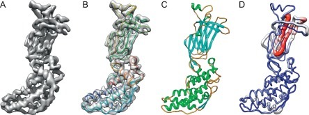
Modeling a 3.8 Å cryoEM map of VP6 of rotavirus. (A) A segmented density map of a capsid protein subunit of rotavirus (VP6) determined at 3.8 Å (EMDB1460). (B) A de novo model built by pathwalker superimposed on the density map. (C) A crystal structure of the same protein (PDB 1QHD). (D) A Cα rms deviation between the cryoEM model and crystal structure with the most and least deviation in red (gray in the print version) and blue (dark gray in the print version), respectively.

These figures are kindly provided by Matthew L. Baker reproduced after Baker M.R. et al. (2012).

While many cryoEM structural models have been built solely using one of the above approaches, some of the more recent structures are large, complex, and have variable resolution throughout the map, necessitating the use of multiple modeling techniques. For instance, the inositol-1,4,5-trisphosphate receptor (IP3R1), a tetrameric cation channel, has 10 discrete structural domains arranged over 2750 amino acids per polypeptide chain (Fan et al., 2015). Among these domains, only ~ 600 residues have a corresponding high-resolution crystallographic structure. Building a model of such a large protein (Fig. 5 ) requires the use of a cocktail of modeling methods including sequence prediction (Cole et al., 2008, Kelley and Sternberg, 2009), secondary structure element localization (Baker et al., 2007), homology modeling (Topf et al., 2006, Webb and Sali, 2014), rigid body and flexible fitting (Jiang et al., 2001, Pettersen et al., 2004, Wriggers and Chacon, 2001), and de novo modeling (Baker, Baker, et al., 2012, Baker, Rees, et al., 2012, Emsley et al., 2010). As such, modeling of these types of complexes requires a more complex strategy that integrates the various software packages and utilizes other structural data. Such integrative methods will likely prove commonplace as cryoEM is applied to large multisubunit molecular machines.

Fig. 5.

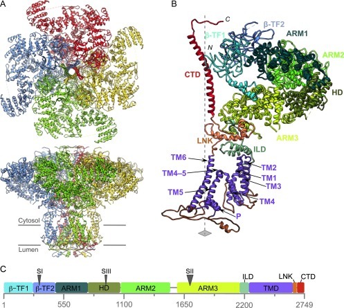
Modeling IP3R1 from a 4.7 Å cryoEM map (EMDB6369) (Fan et al., 2015). (A) The model (PDB 3JAV) was built using a variety of modeling protocols, shown from two views. The model is of the entire tetramer with 85% chain connectivity per chain, partly due to the presence of isoforms at the SI, SII, and SIII sites causing specimen heterogeneity and partly due to the limited map resolution. (B) The annotation of the 10 structural domains of a single IP3R1 subunit with 2700 amino acids. (C) A schematic of the corresponding domains in the linear sequence.

Reproduced from Fan, G., Baker, M. L., Wang, Z., Baker, M. R., Sinyagovskiy, P. A., Chiu, W., et al. (2015). Gating machinery of InsP3R channels revealed by electron cryomicroscopy. Nature, 527, 336–341 and provided by Matthew L. Baker.

3. Model Optimization

Once an initial model is constructed, or if a high-resolution homologous structure is already known, the next step in structure determination is model optimization. In this case, the task is to move atom positions to improve agreement to data, improve model geometry (eg, eliminating clashes and unreasonable torsions), or some combination of both. Specifically, this step aims to optimize protein coordinates to minimize a target function $E=E_{\mathrm{geom}}+w\cdot E_{\mathrm{data}}$, where E _geom assesses the geometric goodness of a model, E _data assesses model-map agreement, and w is a weighing factor controlling the relative contributions of geometry and agreement to data in optimization. This section describes a number of different tools for model optimization, which vary in the functional form of E _geom and E _data, the parameter space describing protein motion, and the types of movements used to optimize E. Consequently, these methods may vary quite a bit in terms of recommended resolutions, magnitude of movements, and runtime of the corresponding approaches. This section gives an overview of each of these methods, when they may best be used and how to interpret the resulting output.

As with the de novo section above, several of the tools commonly used in model refinement are based on tools originally developed for X-ray crystallography. In particular, both Phenix.refine (Afonine et al., 2012) and Refmac have been commonly used (eg, phenix.refine was used to refine the first cryoEM structure of epsilon15 bacteriophage capsid (Baker et al., 2013)). In using these crystallographic tools, the data are first processed as if it were crystal data, assigning an artificial unit cell and symmetry to the data, and computing reciprocal space intensities and phases from the real-space density. Then, refinement is carried against a function that takes into account both Fourier intensities and phases of the data. The geometry function used by both is a relatively simple macromolecular energy function that takes into account stereochemistry and steric clashes, with optional support for torsional potentials or user-defined “restraints.” Generally, function optimization consists of cycles of minimization, but may also include discrete rotamer optimization or cycles of simulated annealing. Consequently, these refinement methods are fast, but tend to make relatively small motions from the starting model, leading to a small “radius of convergence”; that is they are unable to correct errors in the starting model of large magnitude. However, they are quite widely used to improve model geometry and improve fit of models to data.

Much like the use of crystallographic tools for de novo model building, one weakness of these tools is that they may not perform particularly well when used at medium-high resolutions. However, there have been a number of recent advances for refinement against low-resolution data. One such approach employs secondary structure element restraints (Nicholls, Long, & Murshudov, 2012), where secondary structure elements in the initial model are identified, and harmonic constraints are used to maintain backbone hydrogen bond patterning throughout optimization, ensuring backbone hydrogen bond patterning stays intact even as refinement moves the structure far from the starting point. Alternately, some approaches make use of “reference-model restraints,” where atom-pair distances or torsions from a related high-resolution structure are applied, rigidifying the structure during the course of optimization (Headd et al., 2012). In this way, refinement fills in ambiguity in the experimental data by enforcing agreement with high-resolution crystallographic data of a related structure. In both approaches, one can think of the restraints as adding additional restraints into E _geom in the equation above.

Several methods have been developed to perform model optimization in real space instead. One advantage of real-space optimization is “locality”: if a map contains contaminants not present in the model (eg, detergents or amphipoles), when the data are converted to reciprocal space, these contaminants will affect the entirety of reciprocal space, but only the affected regions when refining in real space (Brunger & Rice, 1997), as local regions in real space contribute globally in reciprocal space. Similar advantages in real-space optimization arise when optimization is carried out with only partial models. This effect may be ameliorated by masking relevant regions before converting the data to reciprocal space, but this requires that a mask be defined a priori. Much like the crystallographic methods, these approaches also need methods to deal with the relatively low resolution of the data, typically using the same additional terms outlined earlier, improving the sensitivity of E _geom.

One such real-space optimization routine is based on the phenix crystallographic refinement software, called phenix.real_space_refine. This optimization protocol ensures optimal fit-to-density, while maintaining good stereochemistry and rotamer assignments. It is very efficient (generally taking minutes or less even for very large systems) but suffers from the same limitation (of having a small radius of convergence) as its crystallographic counterpart. One recent example where this approach was successfully employed was in structure determination of the brome mosaic virus: an all-atom model was optimized into a 3.8 Å cryoEM density map, resulting in outstanding MolProbity statistics (Chen et al., 2010) compared to the input model or the previously determined 3.4 Å X-ray crystal structure of the same virus particle (Wang et al., 2014) (Table 1 ).

Table 1.

MolProbity Statistics Comparing the cryoEM Map-Derived Models of Brome Mosaic Virus Before and After Real-Space Optimization (RSO) (PDB 3J7L) and the Corresponding X-ray Structure (PDB 1JS9) (Wang et al., 2014)

Asymmetric Unit	3 Subunits	CryoEM 477 Residues at 3.8 Å Resolution After RSO		CryoEM 477 Residues at 3.8 Å Resolution Before RSO		X-ray (PDB id: 1JS9) 503 Residues at 3.4 Å Resolution
Density agreement	Correlation coefficient	0.84		0.76		0.68
All-atom contacts	Clash score (all atoms)	13.35	97th Percentile	16.02	97th Percentile	31.77	78th Percentile
Protein geometry	Poor rotamers	0	0%	172	46%	181	49%
	Ramachandran Outliers	12	2.55%	48	10%	44	9%
	Ramachandran favored	434	92.14%	345	69%	351	71%
	MolProbity score	2.11	100th Percentile	3.82	46th Percentile	4.1	21st Percentile
	Cβ deviations	0	0%	0	0%	0	0%
	Bad backbone bonds	0	0%	1	0.05%	0	0%
	Bad backbone angles	0	0%	8	0.32%	5	0.2%

Percentile values in the table based on deposited structures at the reported resolution.

A complete asymmetric unit was analyzed, but the number of amino acids varies due to resolvability in the density map (EMDB6000). In addition, cross-correlation values were computed between the map and the model for the asymmetric unit. Percentiles were calculated based on the deposited structures at the reported resolution.

Another real-space optimization tool makes use of Rosetta (DiMaio et al., 2015). By replacing the relatively coarse-grained crystallographic E _geom with a richer, physically realistic potential that accounts for the hydrophobic effect, hydrogen bonding, electrostatics, and torsional preferences, the number of effective degrees of freedom during optimization is dramatically limited. This allows for optimization to move the structure significantly while energetically favorable interactions are maintained. Rosetta-based optimization makes use of a combination of minimization and Monte Carlo sampling of both backbone and sidechain conformations, where extensive minimization after each Monte Carlo sampling step allows exploration of a relatively large portion of conformational space. This sampling and energy function allow for larger conformational changes during optimization, however, it also comes at increased computational cost. One further advantage of Rosetta is the symmetric degrees of freedom are explicitly represented rather than restrained with noncrystallographic symmetry restraints. This further reduces degrees of freedom as well as improving performance on very highly symmetric systems (for example, icosahedral viral capsids). An example of the types of movement that may be obtained from this optimization protocol is shown in Fig. 6 .

Fig. 6.

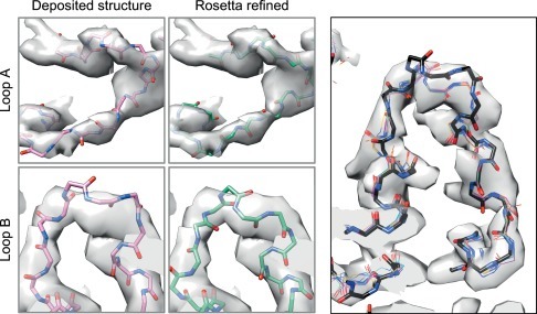
The types of motion possible during Rosetta optimization. (Left) Two different regions of relatively low local resolution in the 3.4 Å resolution map of TRPV1; Rosetta refinement (right two panels) allows for significant conformational difference from the deposited structure (left two panels). (Right) Despite the significant backbone movement in the course of optimization, an ensemble of low energy models, resulting from independent trajectories, are well converged.

Another tool, DireX (Schroder, Levitt, & Brunger, 2010), uses ideas from crystallographic refinement methods as well, but instead is applied in real space, and—to address the poor data-to-parameters ratio of typical crystal refinement—makes use of reference model restraints. However, unlike typical crystallographic refinement programs, these restraints are allowed to change during the course of model optimization. The restraints very slowly adapt to the current model in the course of model optimization, with two metaparameters describing the “stiffness” and “speed” at which these constraints adapt. By exploring the results of refinement over various settings of these metaparameters, an optimal setting may be identified. A key advantage of these adaptable constraints is that they identify a “minimally perturbed conformation,” only violating constraints in the initial model if there is sufficient evidence from the data that these constraints should not hold. Consequently, the approach can allow for relatively large motions during optimization and often works reasonably well at low resolution if a corresponding high-resolution structure is known (Chen, Madan, et al., 2013). Fig. 7 illustrates an application of this approach in the determination of several different forms of F-actin refined against cryoEM data (Galkin et al., 2015).

Fig. 7.

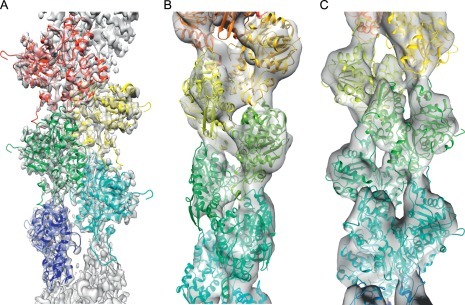
An example of model optimization using DireX to model distinct conformational states of F-actin from a 4.8 Å cryoEM map (Galkin, Orlova, Vos, Schroder, & Egelman, 2015). (A) A 4.8 Å resolution reconstruction of F-actin (EMDB6179) into which a model has been built and optimized (PDB 3J8I). (B and C) Two alternate, low-occupancy conformations of actin, titled T1 and T2, into which the initial model has been refined. Even though the data are of relatively low resolution, DireX attempts to maintain as many contacts as possible during refinement.

Another class of tools is based on molecular dynamics guided by experimental data. The most commonly used tool is MDFF (Trabuco, Villa, Mitra, Frank, & Schulten, 2008), which combines the VMD molecular dynamics package with a score term assessing the agreement of a model to real-space density. Like Rosetta, the rich, physically realistic force field makes the approach well suited to modeling large conformational changes, as it maintains physically realistic geometry. One weakness of this approach is that it may be time consuming, particularly if explicit solvent molecules are used, due to the increased number of interactions introduced by explicit solvent molecules and the long equilibration time consequently necessary. However, it may be parallelized to run in a reasonable amount of wall clock time. To date, it is often preferred for modeling large conformational changes subject to medium-resolution density maps, as in the ribosome (Trabuco et al., 2008) and HIV capsid (Zhao et al., 2013).

Finally, FlexEM is another method that approaches the problem hierarchically (Topf et al., 2008). A protein system is first broken into rigid bodies, which are refined, and then full flexibility is allowed. The score function used is similar to that of crystallographic force fields, however, the initial rigid-body refinement step has relatively few parameters, and thus allows for large motions of the system.

4. Model Validation

Once after model optimization is completed, the final steps are model selection and model validation. Model validation attempts to assess the accuracy of the refined model. This is desirable for several reasons, and model validation may be used to address several different questions that arise during model building. One may want to estimate the absolute accuracy of a model fit to data. Alternately, one may want to compare models to find the most accurate, either to select models from stochastic refinement trajectories, or to tune parameters of model building, such as the weight on the experimental data in refinement. Finally, one may wish to see if the model is improved following optimization and identify when optimization can be stopped (if there is no more improvement).

This section is broadly divided into two parts: validation using model geometry and validation using model-map agreement. However, for both measures, a key to validating models is the use of independent data, that is, data that is not used in optimization—not optimized against—in order to evaluate accuracy of a model. While the agreement of model to data used in fitting is informative, it does not identify overfitting, fitting to noise in the original reconstruction. To identify overfitting, independent data are required (DiMaio, Zhang, Chiu, & Baker, 2013). This is critically important at near-atomic resolutions, as—at these resolutions—it is much easier to trace models incorrectly that fit the data well. Only by assessing the agreement to independent data can we be sure that we are improving the model.

MolProbity, a widely used model validation metric used in both crystallography and with NMR-derived models, assesses the geometry of a protein model (Chen et al., 2010). More specifically, it looks at certain geometric features of a model and compares them to the expected values of such features, as derived from very high-resolution crystal structures. Such features include bond-length and bond-angle distributions, backbone torsional distributions (specifically, counting the number of “allowed” and “favored” backbone dihedrals, which are seen in < 2% and < 0.05% of residues in high-resolution structures, respectively), sidechain rotamer distributions (counting the number of rotamers seen with < 0.3% frequency in high-resolution structures), and atom pairs closer than the sum of their van der Waals radii. For each metric, a corresponding Z-score is computed, and linear regression is used to compute an aggregate score. This aggregate score is trained to predict the resolution of data at which a particular structure was solved using only the geometry of the model itself. The resulting “MolProbity score” can very loosely be thought of in terms of map resolution, where models scoring under 2 are of high quality, while models scoring higher than 4 are of relatively low quality. MolProbity reports (Chen et al., 2010) also describe the ranking of the examined structure relative to all the other structures in the PDB determined at the equivalent resolution (Table 1).

It is also important to point out that for many of the model optimization methods outlined in the previous section, the geometric data are not considered “independent data” for the purposes of validation. Both Rosetta and phenix.refine (when run in a certain mode) restrain sidechains to rotameric identity for example. This is not a weakness of these approaches; indeed, at low resolution such incorporation may be necessary, and given two otherwise equivalent models, the one with better geometry is more likely to be correct. However, for these approaches it is important to realize that these measures are not independent data for assessing overfitting or for parameter tuning.

One may also want to validate models based on fit between model and experimental data. This is often done by evaluating the Fourier shell correlation (FSC) between a model and the corresponding map, quantifying the fit by calculating the correlation between model and map in reciprocal space, in the complex plane. One advantage of this measure over something like real-space correlation is that the measure is independent of dampened intensities in high-resolution shells (real-space correlation is sensitive to this effect). This measure is often computationally corrected during the reconstruction process, and so an assessment measure that ignores this is preferred. In the near-atomic resolution regime, the FSC in high-resolution shells alone is most informative as to the accuracy of the high-resolution details of the model (DiMaio et al., 2015).

There are several different ways in which this measure is used to generate an independent validation measure. All compute a “free FSC” analogous to the R _free measure in X-ray crystallography: the agreement of model and map on a subset of data held aside during refinement. In crystallography, the R _free measure omits a subset (generally 5–10%) of reciprocal space intensities from refinement and evaluates their agreement to the model as refinement progresses. Since it is now a common practice to produce two independent maps from two independent sets of raw particle images to assess map resolution (Chen et al., 2013, Henderson et al., 2012), one can generate two independent models from the two independent maps. These two independent models can be compared against the two maps by either FSC or variance of the backbone between the two models (Rosenthal & Henderson, 2003). In addition, one can compute the FSC between the model derived from one map relative to the other independently determined map (Wang et al., 2014). It has been shown that FSC equal to 0.5 is a practical measure of the agreement between the model and map. If this measure exceeds the gold standard map resolution (Henderson et al., 2012, Scheres and Chen, 2012), it would imply that the model is overfitted. These multiple crosschecks should provide consistent results to assure that the model is not overfitted in each case. Fig. 8 shows an example application of this model validation metric in the 3.8 Å cryoEM structure of brome mosaic virus (Wang et al., 2014). This validation approach is additionally informative for tuning the relative weight of experimental data and geometric data during the optimization process. It is very much analogous to the R _free measure in X-ray crystallography: the agreement of model and map on a subset of data held aside during refinement. To deal with the somewhat reduced resolution, it is also proposed to perform additional refinement against the reconstruction of the entire data set (Brown et al., 2015), however, this final refinement is no longer independent with respect to the “independent map.”

Fig. 8.

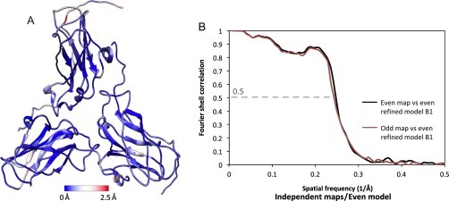
Model validation of a 3.8 Å cryoEM map of brome mosaic virus (EMDB6000) (Wang et al., 2014) by (A) deviation between two independent models at the Cα level (PDB 3J7M and PDB 3J7N). (B) FSC between model and experimental map from two independent data sets.

These figures are reproduced from Wang, Z., Hryc, C. F., Bammes, B., Afonine, P. V., Jakana, J., Chen, D. H., et al. (2014). An atomic model of brome mosaic virus using direct electron detection and real-space optimization. Nature Communications, 5, 4808 and kindly provided by Corey F. Hryc.

Alternatively, another approach (Falkner & Schroder, 2013), rather than using two different reconstructions, instead truncates the full reconstruction at some particular resolution (at the point where the FSC of two independent maps is 0.5). Fitting is carried out against this truncated reconstruction, while the truncated high-resolution information is used as an independent validation set. The advantage of the latter approach is that independent maps are not required. However, both techniques have been successfully employed in order to detect overfitting.

A final method for map validation, EMRinger (Barad et al., 2015), also comes from X-ray crystallography. This method, outlined in Fig. 9 , identifies the fraction of amino acids with “rotameric sidechain density.” While conceptually it may seem to be similar to rotamer probabilities reported by MolProbity, it actually is quite different. It measures whether density is rotameric for a particular sidechain, that is, by looking along the Cα–Cβ vector of each residue, and identifying if the putative Cγ peak is rotameric. In doing so, it ignores whether the modeled sidechain is actually rotameric. Instead, it identifies backbone placements where sidechain density seems reasonable; incorrectly placed backbone will have nonrotameric sidechain density, even if the modeled sidechain is rotameric. Important to note is that this measure only depends upon the placement of backbone atoms, and it can be thought of as an orthogonal measure to those above.

Fig. 9.

(A) A schematic of the use of EMRinger for model validation (Barad et al., 2015). Given a backbone model and a density map, EMRinger considers all possible positions for a putative Cγ and identifies density peaks at a given threshold; the fractions of these peaks over the whole structure, which are rotameric are used to assess the quality of the model. (B) The results of EMRinger analysis on a sample system: the x-axis plots various density value cutoffs and the y-axis shows the EMRinger Z-score. Higher values are better, with Z-score of > 2 indicating high-quality structures.

These figures are reproduced from Barad, B. A., Echols, N., Wang, R. Y., Cheng, Y., DiMaio, F., Adams, P. D., et al. (2015). EMRinger: Side chain-directed model and map validation for 3D cryo-electron microscopy. Nature Methods, 12, 943–946.

5. Discussion

This review provides a detailed view of the steps required in going from a cryoEM map to all-atom model. As illustrated, there are a wide variety of tools, each with tradeoffs in terms of most effective resolutions, run time, conformational state explored. However, these methods show that it is possible to obtain accurate, all-atom reconstructions from cryoEM density.

We have primarily focused on the determination of a single model that best explains the data. However, the reality is that—as an averaging method—a single cryoEM reconstruction may contain many different conformations of individual molecules. It might then make sense to consider fitting ensembles of models to cryoEM reconstructions. However, as X-ray crystallographic methods show us (Terwilliger et al., 2012), it is difficult to do this for two reasons: it introduces a significant number of parameters to optimization, and it is difficult to separate out the effects of uncertainty from conformational variability. An open challenge in future years remains how to represent and validate the various conformations possibly seen in different frequencies in a single molecular machine.

Finally, with the relatively low resolution of cryoEM reconstructions compared to those in crystallography, it is important to assess the accuracy of computed models. This is commonly done in several ways: by exploring the space of solutions consistent with data (DiMaio et al., 2015), by looking at consistency in models fit to independent datasets (DiMaio et al., 2013, Wang et al., 2014), and by explicitly fitting models that contain uncertainty (Pintilie, Chen, Haase-Pettingell, King, & Chiu, 2016), essentially putting error bars on generated models. The question is still an open one; however, as there is no consensus on the best way to compute or to represent uncertainty of a model given a reconstruction. So far, all the modeling is based on the assumption of the density map being correct and having an isotropic resolution. It has been shown in numerous cases that resolutions are nonuniform throughout the map. It will be very important in the future to explore this problem more rigorously. Accounting for the uncertainty of the model and the map is key to interpreting the biology of the corresponding system and planning next set of experiments based on the structures.

References

- Adams P.D., Afonine P.V., Bunkoczi G., Chen V.B., Davis I.W., Echols N. PHENIX: A comprehensive Python-based system for macromolecular structure solution. Acta Crystallographica. Section D, Biological Crystallography. 2010;66:213–221. doi: 10.1107/S0907444909052925. [DOI] [PMC free article] [PubMed] [Google Scholar]
- Afonine P.V., Grosse-Kunstleve R.W., Echols N., Headd J.J., Moriarty N.W., Mustyakimov M. Towards automated crystallographic structure refinement with phenix.refine. Acta Crystallographica. Section D, Biological Crystallography. 2012;68:352–367. doi: 10.1107/S0907444912001308. [DOI] [PMC free article] [PubMed] [Google Scholar]
- Baker M.L., Abeysinghe S.S., Schuh S., Coleman R.A., Abrams A., Marsh M.P. Modeling protein structure at near atomic resolutions with Gorgon. Journal of Structural Biology. 2011;174:360–373. doi: 10.1016/j.jsb.2011.01.015. [DOI] [PMC free article] [PubMed] [Google Scholar]
- Baker M.L., Baker M.R., Hryc C.F., Ju T., Chiu W. Gorgon and pathwalking: Macromolecular modeling tools for subnanometer resolution density maps. Biopolymers. 2012;97:655–668. doi: 10.1002/bip.22065. [DOI] [PMC free article] [PubMed] [Google Scholar]
- Baker M.L., Hryc C.F., Zhang Q., Wu W., Jakana J., Haase-Pettingell C. Validated near-atomic resolution structure of bacteriophage epsilon15 derived from cryo-EM and modeling. Proceedings of the National Academy of Sciences of the United States of America. 2013;110:12301–12306. doi: 10.1073/pnas.1309947110. [DOI] [PMC free article] [PubMed] [Google Scholar]
- Baker M.L., Ju T., Chiu W. Identification of secondary structure elements in intermediate-resolution density maps. Structure. 2007;15:7–19. doi: 10.1016/j.str.2006.11.008. [DOI] [PMC free article] [PubMed] [Google Scholar]
- Baker M.R., Rees I., Ludtke S.J., Chiu W., Baker M.L. Constructing and validating initial Calpha models from subnanometer resolution density maps with pathwalking. Structure. 2012;20:450–463. doi: 10.1016/j.str.2012.01.008. [DOI] [PMC free article] [PubMed] [Google Scholar]
- Barad B.A., Echols N., Wang R.Y., Cheng Y., DiMaio F., Adams P.D. EMRinger: Side chain-directed model and map validation for 3D cryo-electron microscopy. Nature Methods. 2015;12:943–946. doi: 10.1038/nmeth.3541. [DOI] [PMC free article] [PubMed] [Google Scholar]
- Brown A., Long F., Nicholls R.A., Toots J., Emsley P., Murshudov G. Tools for macromolecular model building and refinement into electron cryo-microscopy reconstructions. Acta Crystallographica. Section D, Biological Crystallography. 2015;71:136–153. doi: 10.1107/S1399004714021683. [DOI] [PMC free article] [PubMed] [Google Scholar]
- Brunger A.T., Rice L.M. Crystallographic refinement by simulated annealing: Methods and applications. Methods in Enzymology. 1997;277:243–269. doi: 10.1016/s0076-6879(97)77015-0. [DOI] [PubMed] [Google Scholar]
- Chen V.B., Arendall W.B., 3rd, Headd J.J., Keedy D.A., Immormino R.M., Kapral G.J. MolProbity: All-atom structure validation for macromolecular crystallography. Acta Crystallographica. Section D, Biological Crystallography. 2010;66:12–21. doi: 10.1107/S0907444909042073. [DOI] [PMC free article] [PubMed] [Google Scholar]
- Chen M., Baldwin P. R., Ludtke S. J., & Baker M. L. (2016). De novo modeling of cryo-EM density maps with pathwalker, Journal of Structural Biology, (in press). [DOI] [PMC free article] [PubMed]
- Chen D.H., Madan D., Weaver J., Lin Z., Schroder G.F., Chiu W. Visualizing GroEL/ES in the act of encapsulating a folding protein. Cell. 2013;153:1354–1365. doi: 10.1016/j.cell.2013.04.052. [DOI] [PMC free article] [PubMed] [Google Scholar]
- Chen S., McMullan G., Faruqi A.R., Murshudov G.N., Short J.M., Scheres S.H. High-resolution noise substitution to measure overfitting and validate resolution in 3D structure determination by single particle electron cryomicroscopy. Ultramicroscopy. 2013;135C:24–35. doi: 10.1016/j.ultramic.2013.06.004. [DOI] [PMC free article] [PubMed] [Google Scholar]
- Cole C., Barber J.D., Barton G.J. The Jpred 3 secondary structure prediction server. Nucleic Acids Research. 2008;36:W197–W201. doi: 10.1093/nar/gkn238. [DOI] [PMC free article] [PubMed] [Google Scholar]
- Cowtan K. The Buccaneer software for automated model building. 1. Tracing protein chains. Acta Crystallographica. Section D, Biological Crystallography. 2006;62:1002–1011. doi: 10.1107/S0907444906022116. [DOI] [PubMed] [Google Scholar]
- DiMaio F., Song Y., Li X., Brunner M.J., Xu C., Conticello V. Atomic-accuracy models from 4.5-A cryo-electron microscopy data with density-guided iterative local refinement. Nature Methods. 2015;12:361–365. doi: 10.1038/nmeth.3286. [DOI] [PMC free article] [PubMed] [Google Scholar]
- DiMaio F., Zhang J., Chiu W., Baker D. Cryo-EM model validation using independent map reconstructions. Protein Science: A Publication of the Protein Society. 2013;22:865–868. doi: 10.1002/pro.2267. [DOI] [PMC free article] [PubMed] [Google Scholar]
- Emsley P., Lohkamp B., Scott W.G., Cowtan K. Features and development of Coot. Acta Crystallographica. Section D, Biological Crystallography. 2010;66:486–501. doi: 10.1107/S0907444910007493. [DOI] [PMC free article] [PubMed] [Google Scholar]
- Falkner B., Schroder G.F. Cross-validation in cryo-EM-based structural modeling. Proceedings of the National Academy of Sciences of the United States of America. 2013;110:8930–8935. doi: 10.1073/pnas.1119041110. [DOI] [PMC free article] [PubMed] [Google Scholar]
- Fan G., Baker M.L., Wang Z., Baker M.R., Sinyagovskiy P.A., Chiu W. Gating machinery of InsP3R channels revealed by electron cryomicroscopy. Nature. 2015;527:336–341. doi: 10.1038/nature15249. [DOI] [PMC free article] [PubMed] [Google Scholar]
- Galkin V.E., Orlova A., Vos M.R., Schroder G.F., Egelman E.H. Near-atomic resolution for one state of F-actin. Structure. 2015;23:173–182. doi: 10.1016/j.str.2014.11.006. [DOI] [PMC free article] [PubMed] [Google Scholar]
- Headd J.J., Echols N., Afonine P.V., Grosse-Kunstleve R.W., Chen V.B., Moriarty N.W. Use of knowledge-based restraints in phenix.refine to improve macromolecular refinement at low resolution. Acta Crystallographica. Section D, Biological Crystallography. 2012;68:381–390. doi: 10.1107/S0907444911047834. [DOI] [PMC free article] [PubMed] [Google Scholar]
- Henderson R. Overview and future of single particle electron cryomicroscopy. Archives of Biochemistry and Biophysics. 2015;581:19–24. doi: 10.1016/j.abb.2015.02.036. [DOI] [PubMed] [Google Scholar]
- Henderson R., Sali A., Baker M.L., Carragher B., Devkota B., Downing K.H. Outcome of the first electron microscopy validation task force meeting. Structure. 2012;20:205–214. doi: 10.1016/j.str.2011.12.014. [DOI] [PMC free article] [PubMed] [Google Scholar]
- Jiang W., Baker M.L., Jakana J., Weigele P.R., King J., Chiu W. Backbone structure of the infectious epsilon15 virus capsid revealed by electron cryomicroscopy. Nature. 2008;451:1130–1134. doi: 10.1038/nature06665. [DOI] [PubMed] [Google Scholar]
- Jiang W., Baker M.L., Ludtke S.J., Chiu W. Bridging the information gap: Computational tools for intermediate resolution structure interpretation. Journal of Molecular Biology. 2001;308:1033–1044. doi: 10.1006/jmbi.2001.4633. [DOI] [PubMed] [Google Scholar]
- Kelley L.A., Sternberg M.J. Protein structure prediction on the Web: A case study using the Phyre server. Nature Protocols. 2009;4:363–371. doi: 10.1038/nprot.2009.2. [DOI] [PubMed] [Google Scholar]
- Kudryashev M., Wang R.Y., Brackmann M., Scherer S., Maier T., Baker D. Structure of the type VI secretion system contractile sheath. Cell. 2015;160:952–962. doi: 10.1016/j.cell.2015.01.037. [DOI] [PMC free article] [PubMed] [Google Scholar]
- Kuhlbrandt W. Biochemistry. The resolution revolution. Science. 2014;343:1443–1444. doi: 10.1126/science.1251652. [DOI] [PubMed] [Google Scholar]
- Lasker K., Topf M., Sali A., Wolfson H.J. Inferential optimization for simultaneous fitting of multiple components into a CryoEM map of their assembly. Journal of Molecular Biology. 2009;388:180–194. doi: 10.1016/j.jmb.2009.02.031. [DOI] [PMC free article] [PubMed] [Google Scholar]
- Lindert S., Staritzbichler R., Wotzel N., Karakas M., Stewart P.L., Meiler J. EM-fold: De novo folding of alpha-helical proteins guided by intermediate-resolution electron microscopy density maps. Structure. 2009;17:990–1003. doi: 10.1016/j.str.2009.06.001. [DOI] [PMC free article] [PubMed] [Google Scholar]
- Nicholls R.A., Long F., Murshudov G.N. Low-resolution refinement tools in REFMAC5. Acta Crystallographica. Section D, Biological Crystallography. 2012;68:404–417. doi: 10.1107/S090744491105606X. [DOI] [PMC free article] [PubMed] [Google Scholar]
- Pettersen E.F., Goddard T.D., Huang C.C., Couch G.S., Greenblatt D.M., Meng E.C. UCSF Chimera—A visualization system for exploratory research and analysis. Journal of Computational Chemistry. 2004;25:1605–1612. doi: 10.1002/jcc.20084. [DOI] [PubMed] [Google Scholar]
- Pintilie G.D., Chen D.H., Haase-Pettingell C.A., King J.A., Chiu W. Resolution and probabilistic models of components in CryoEM maps of mature P22 bacteriophage. Biophysical Journal. 2016;110:827–839. doi: 10.1016/j.bpj.2015.11.3522. [DOI] [PMC free article] [PubMed] [Google Scholar]
- Pintilie G., Zhang J., Chiu W., Gossard D. Identifying components in 3D density maps of protein nanomachines by multi-scale segmentation. IEEE/NIH Life Science Systems and Applications Workshop. 2009;2009:44–47. doi: 10.1109/LISSA.2009.4906705. [DOI] [PMC free article] [PubMed] [Google Scholar]
- Pintilie G.D., Zhang J., Goddard T.D., Chiu W., Gossard D.C. Quantitative analysis of cryo-EM density map segmentation by watershed and scale-space filtering, and fitting of structures by alignment to regions. Journal of Structural Biology. 2010;170:427–438. doi: 10.1016/j.jsb.2010.03.007. [DOI] [PMC free article] [PubMed] [Google Scholar]
- Rosenthal P.B., Henderson R. Optimal determination of particle orientation, absolute hand, and contrast loss in single-particle electron cryomicroscopy. Journal of Molecular Biology. 2003;333:721–745. doi: 10.1016/j.jmb.2003.07.013. [DOI] [PubMed] [Google Scholar]
- Scheres S.H., Chen S. Prevention of overfitting in cryo-EM structure determination. Nature Methods. 2012;9:853–854. doi: 10.1038/nmeth.2115. [DOI] [PMC free article] [PubMed] [Google Scholar]
- Schroder G.F., Levitt M., Brunger A.T. Super-resolution biomolecular crystallography with low-resolution data. Nature. 2010;464:1218–1222. doi: 10.1038/nature08892. [DOI] [PMC free article] [PubMed] [Google Scholar]
- Terwilliger T.C., Read R.J., Adams P.D., Brunger A.T., Afonine P.V., Grosse-Kunstleve R.W. Improved crystallographic models through iterated local density-guided model deformation and reciprocal-space refinement. Acta Crystallographica. Section D, Biological Crystallography. 2012;68:861–870. doi: 10.1107/S0907444912015636. [DOI] [PMC free article] [PubMed] [Google Scholar]
- Topf M., Baker M.L., Marti-Renom M.A., Chiu W., Sali A. Refinement of protein structures by Iterative comparative modeling and cryoEM density fitting. Journal of Molecular Biology. 2006;357:1655–1668. doi: 10.1016/j.jmb.2006.01.062. [DOI] [PubMed] [Google Scholar]
- Topf M., Lasker K., Webb B., Wolfson H., Chiu W., Sali A. Protein structure fitting and refinement guided by Cryo-EM density. Structure. 2008;16:295–307. doi: 10.1016/j.str.2007.11.016. [DOI] [PMC free article] [PubMed] [Google Scholar]
- Trabuco L.G., Villa E., Mitra K., Frank J., Schulten K. Flexible fitting of atomic structures into electron microscopy maps using molecular dynamics. Structure. 2008;16:673–683. doi: 10.1016/j.str.2008.03.005. [DOI] [PMC free article] [PubMed] [Google Scholar]
- Walls A.C., Tortorici M.A., Bosch B.J., Frenz B., Rottier P.J., DiMaio F. Cryo-electron microscopy structure of a coronavirus spike glycoprotein trimer. Nature. 2016;531:114–117. doi: 10.1038/nature16988. [DOI] [PMC free article] [PubMed] [Google Scholar]
- Wang Z., Hryc C.F., Bammes B., Afonine P.V., Jakana J., Chen D.H. An atomic model of brome mosaic virus using direct electron detection and real-space optimization. Nature Communications. 2014;5:4808. doi: 10.1038/ncomms5808. [DOI] [PMC free article] [PubMed] [Google Scholar]
- Wang R.Y., Kudryashev M., Li X., Egelman E.H., Basler M., Cheng Y. De novo protein structure determination from near-atomic-resolution cryo-EM maps. Nature Methods. 2015;12:335–338. doi: 10.1038/nmeth.3287. [DOI] [PMC free article] [PubMed] [Google Scholar]
- Webb B., Sali A. Comparative protein structure modeling using MODELLER. Current Protocols in Bioinformatics/Editoral Board, Andreas D Baxevanis [et al.] 2014;47:5.6.1–5.6.32. doi: 10.1002/0471250953.bi0506s47. [DOI] [PubMed] [Google Scholar]
- Wriggers W., Chacon P. Modeling tricks and fitting techniques for multiresolution structures. Structure. 2001;9:779–788. doi: 10.1016/s0969-2126(01)00648-7. [DOI] [PubMed] [Google Scholar]
- Zhao G., Perilla J.R., Yufenyuy E.L., Meng X., Chen B., Ning J. Mature HIV-1 capsid structure by cryo-electron microscopy and all-atom molecular dynamics. Nature. 2013;497:643–646. doi: 10.1038/nature12162. [DOI] [PMC free article] [PubMed] [Google Scholar]