Abstract
Positron emission tomography (PET) images are widely used in many clinical applications such as tumor detection and brain disorder diagnosis. To obtain PET images of diagnostic quality, a sufficient amount of radioactive tracer has to be injected into a living body, which will inevitably increase the risk of radiation exposure. On the other hand, if the tracer dose is considerably reduced, the quality of the resulting images would be significantly degraded. It is of great interest to estimate a standard-dose PET (S-PET) image from a low-dose one in order to reduce the risk of radiation exposure and preserve image quality. This may be achieved through mapping both standard-dose and low-dose PET data into a common space and then performing patch based sparse representation. However, a one-size-fits-all common space built from all training patches is unlikely to be optimal for each target S-PET patch, which limits the estimation accuracy. In this paper, we propose a data-driven multi-level Canonical Correlation Analysis (mCCA) scheme to solve this problem. Specifically, a subset of training data that is most useful in estimating a target S-PET patch is identified in each level, and then used in the next level to update common space and improve estimation. Additionally, we also use multi-modal magnetic resonance images to help improve the estimation with complementary information. Validations on phantom and real human brain datasets show that our method effectively estimates S-PET images and well preserves critical clinical quantification measures, such as standard uptake value.
Keywords: PET estimation, multi-level CCA, sparse representation, locality-constrained linear coding, multi-modal MRI
I. Introduction
POSITRON emission tomography (PET) is a functional imaging technique that is often used to reveal metabolic information for detecting tumors, searching for metastases and diagnosing certain brain diseases [1, 2]. By detecting pairs of gamma rays emitted from the radioactive tracer injected into a living body, the PET scanner generates an image, based on the map of radioactivity of the tracer at each voxel location.
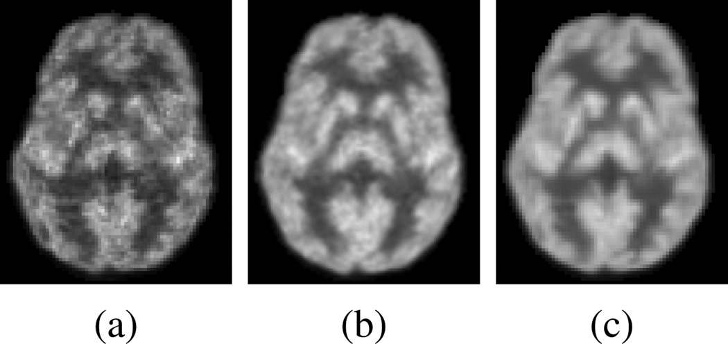
To obtain PET images of diagnostic quality, a standard-dose tracer is often used. However, this raises the risk of radioactive exposure, which can be potentially detrimental to one’s health. Recently, researchers have tried to lower the dose during PET scanning, e.g., using half of the standard dose [3]. Although it is desirable to reduce the dose during the imaging process, reducing the dose will inevitably degrade the overall quality of the PET image. As shown in Fig. 1(a) and (b), the low-dose PET (L-PET) image and the standard-dose (SPET) image differ significantly in image quality, though both images are of the same subject. Our method aims to estimate the S-PET image in a data-driven manner to produce a result (Fig. 1(c)) that is very close to the original S-PET image. Also, since the modern PET scanner is often combined with other imaging modalities (e.g., magnetic resonance imaging (MRI)) to provide both metabolic and anatomical details [4], such information could be leveraged for better estimation of S-PET images.
Fig. 1.
(a) Low-dose PET image of a subject. (b) Standard-dose PET image of the same subject. (c) Estimated standard-dose PET image by our method.
Since PET images often have poor signal-to-noise ratio (SNR) due to the high level of noise and low spatial resolution, there are a lot of works that have been proposed to improve the PET image quality during the reconstruction or the post-reconstruction process. For example, during the reconstruction process, anatomical information from MRI prior [5–7] has been utilized. In [8], a nonlocal regularizer is developed, which can selectively consider the anatomical information only when it is reliable, and this information can come from MRI or CT. In the post-reconstruction process, CT [9, 10] or MRI [11] information can be incorporated. In [12], both CT and MRI are combined in the post-reconstruction process. These methods can suppress noise and improve image quality. Some works have specifically focused on reducing the noise in PET images, including the use of the singular value thresholding concept and Stein’s unbiased risk estimate [13], the use of spatiotem-poral patches in a non-local means framework [14], the joint use of wavelet and curvelet transforms [15], and simultaneous delineation and denoising [16].
The aforementioned methods are mainly developed to improve the PET image quality during the reconstruction or the post-reconstruction process. On the contrary, in this work, we study the possibility of generating S-PET alike image with diagnostic quality from L-PET image and MRI image, and investigate how well the image quantification can be preserved in the estimated S-PET images. Our method is essentially a learning-based mapping approach to infer unknown data from known data in different modalities, in contrast to conventional image enhancement methods.
For practical nuclear medicine, it is desirable to reduce the dose of radioactive tracer. However, lowering radiation dose changes the underlying biological or metabolic process. Therefore, the low-dose and standard-dose PET images can be different in terms of activity. This actually brings the motivation of our method, in which we aim to estimate standard-dose alike PET images from L-PET images, which cannot be achieved by simple post-processing operations such as denoising. To our best knowledge, very few methods attempt to directly estimate the S-PET image from an LPET image, for example, using regression forest [17, 18]. Specifically, in [17] and [18], a regression forest can be trained to estimate a voxel value in an S-PET image, with L-PET voxel values in the neighborhood as input to the RF. The quality of the estimated S-PET images can be further improved by incremental refinement. In the CT imaging domain, to obtain a CT image of diagnostic quality with a lesser dose, Fang et al. [19] proposed a low-dose CT perfusion deconvolution method using tensor total-variation regularization.
Recently there have been rapid development in sparse representation (SR) and dictionary learning for medical images [20]. For example, estimating S-PET image from L-PET image can be achieved in patch-based SR by learning a pair of coupled dictionaries from L-PET and S-PET training patches. It is assumed that both L-PET and S-PET patches lie in the low dimensional manifolds with similar geometry. To estimate a target S-PET patch, its corresponding L-PET patch is first sparsely represented by the L-PET dictionary, which includes a set of training L-PET patches. The resulting reconstruction coefficients are then directly applied to the S-PET dictionary for estimation of S-PET image, where the S-PET dictionary is composed of a set of S-PET patches, each corresponding to an L-PET patch in the L-PET dictionary.
Usually, the patches in the two dictionaries have different distributions (i.e., neighborhood geometry) due to changes in imaging condition. Hence, it is inappropriate to directly apply the learned coefficients from the L-PET dictionary to the S-PET dictionary for estimation. A solution to this problem is to map those patches into a common space before applying sparse coefficients for minimizing their distribution discrepancy. Common space, or sometimes referred to as coherent space, is a feature space where the coherence between the topological structures of data from different modalities (i.e., L-PET and S-PET patches in our case) is established. In this common space, the L-PET and S-PET features share a common topological structure, and thus an S-PET patch can be estimated more accurately by exploiting the geometric structure of the L-PET patches. One popular technique to learn such common space is Canonical Correlation Analysis (CCA) [21], which has been widely applied in various tasks, such as disease classification [22, 23], population studies [24], image registration [25], and medical data fusion [26]. CCA can be used to learn global mapping with the original coupled L-PET and S-PET dictionaries and then map both kinds of data into their common space. However, global common space mapping does not necessarily unify neighborhood structures in the coupled dictionaries that are involved in reconstructing a specific L-PET patch. Hence, it is sub-optimal to estimate its corresponding S-PET patch using the same reconstruction coefficients.
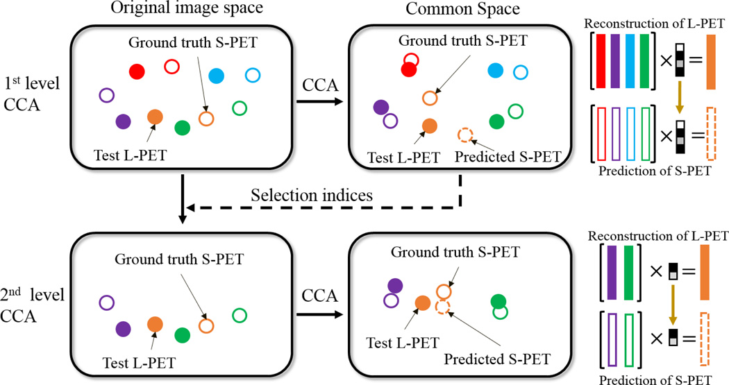
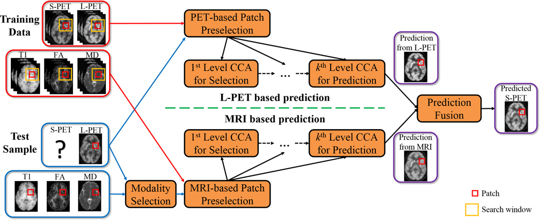
To accurately learn the common space for S-PET estimation, we propose a multi-level CCA (mCCA) framework. Fig. 2 illustrates a two-level scheme. In the first level (top part of Fig. 2), after mapping both L-PET and S-PET data into their common space, a test L-PET patch can be reconstructed by the L-PET dictionary. Rather than immediately estimating the target S-PET patch in this level, a subset of the L-PET dictionary atoms (patches with non-zero coefficients) that are most useful for reconstructing the test L-PET patch are selected and passed on together to the next level with the corresponding S-PET dictionary subset (lower part of Fig. 2). With this data-driven dictionary refinement, the subsequent common space learning and estimation will be improved in the next level. We observe that repeating this process leads to a better final estimation. In addition to the L-PET based estimation, we also leverage multi-modal MRI (i.e., T1-weighted and diffusion tensor imaging (DTI)) to generate an MRI based estimation in a similar way, which can be used to improve the simple L-PET based estimation in a fusion process. This is depicted in Fig. 3. As can be seen, given a test L-PET patch, the training patches are adaptively selected and then used to learn multiple levels of CCA-based common space, with the goal of better representing this test L-PET patch in each level. Similarly, estimation can be made from a test MRI patch (bottom part) by selecting one MRI modality that has the highest correlation with the test L-PET patch. Finally, a fusion strategy generates the final estimated S-PET patch, and all the estimated S-PET patches are aggregated to form the output S-PET image.
Fig. 2.
Illustration of the multi-level CCA scheme (with two levels shown as example). Filled patterns denote L-PET patches and unfilled patterns denote S-PET patches. A pair of L-PET and S-PET patches are indicated by the same color. A coarse reconstruction in the first level (top) is used to select the refined subsets of dictionaries. At this stage, the dictionary atoms that contribute more in reconstructing the test patch are selected. The estimation in the second level (bottom) is more accurate thanks to the improved mapping and reconstruction using the refined dictionaries. Best viewed in color.
Fig. 3.
Our framework for estimating S-PET image from L-PET and MR images. The top part illustrates the proposed multi-level CCA-based estimation from L-PET patches, and the bottom part depicts the same strategy for estimation using MRI as input. In each level, for a particular test patch, a subset of dictionary atoms are adaptively selected and then the refined dictionaries in the original image space are provided to the next level for common space learning and reconstruction. In the final stage, a fusion strategy is adopted to generate the final estimated S-PET patch using both the MRI- and L-PET-based estimations. Best viewed in color.
We note that in a recent work [27], qualitative visual inspections were performed by physicians on whole-body PET images, and no significant difference between PET images with different doses was found. However, it was observed that the standard uptake values (SUVs) have changed when using different doses. In our work, we test our method on both brain phantom data with abnormality (i.e., lesion) and real brain data. Different from [27], we provide quantitative evaluations in terms of both image quality and clinical quantification measures. The results suggest that our estimated standard-dose alike PET images are more similar to the ground-truth standard-dose images, while the low-dose PET images are significantly deviated from standard-dose PET images in various measures.
Compared to [17, 18], in which the PET estimation is formulated as a regression problem, our approach tackles it as a sparse representation problem. The sparse representation is computed in an iteratively-refined common space for L-PET and S-PET images. Because the intra-data relationships in the L-PET and S-PET data spaces are different, a direct coding and estimation step in the original image space would not be optimal. In our approach, the estimation uses the sparse coefficients learned in the common space, which has shown to be more effective through experiments using both image quality and clinical quantification measures. Compared to the results in [18], with the same data and experimental settings, superior performance is achieved by our method. Furthermore, only T1-weighted MRI was used in [18], while in our method, multi-modal MRI can be adaptively selected and utilized for improved estimation as compared to using only T1.
In summary, the contributions of this work are two-fold:
An mCCA based data-driven scheme is developed to estimate an S-PET image from an L-PET counterpart, such that its quality is iteratively refined;
Our framework combines both L-PET and multi-modal MRI for better estimation. To the best of our knowledge, this is the first work that estimates an S-PET image by fusing the information from its low-dose counterpart and multi-modal MR images.
The effectiveness of our proposed method was evaluated on a real human brain image dataset. Extensive experiments were conducted using both image quality metrics and clinical quantification measures. The results demonstrate that the estimated S-PET images well preserve critical measurements such as standard uptake value (SUV) and show the improved image quality in terms of quantitative measures such as peak signal-to-noise ratio (PSNR), as compared to the L-PET images and also the estimations by those baseline methods.
Below we first describe the proposed method in detail in Section II. Then, we show extensive experimental results, evaluated with different metrics, on both phantom brain dataset and real human brain dataset in Section III. Finally, we conclude the paper in Section IV.
II. Methodology
Suppose we have a group of N training image pairs, with each composed of an L-PET image and an S-PET image. Given a target L-PET image, we seek to estimate its S-PET counterpart using the training set in a patch-wise manner. Specifically, we first break down each pair of the training images into a number of patches at corresponding voxels, thus leading to sets of L-PET and associated S-PET training patches. Given a target S-PET patch to be estimated, the training patches within the corresponding neighborhood are extracted and preselected. After learning and refining a common space in multiple levels, an estimate of the target SPET patch from its L-PET counterpart is obtained by patch based SR with the selected training patches. By replacing L-PET with multi-modal MRI and repeating the above process, we can obtain the estimates of the target S-PET patch from multiple modalities. We then fuse those estimates together to obtain the final estimate. Below we elaborate mCCA for L-PET and multi-modal MR based estimation in detail. We use bold lowercase letters (e.g., w) to denote vectors and bold uppercase letters (e.g., W) for matrices. Before diving into details, we first briefly review CCA.
A. Canonical Correlation Analysis (CCA)
First introduced in [21], CCA is a multivariate statistical analysis tool. CCA aims at projecting two sets of multivariate data into a common space such that the correlation between the projected data is maximized.
In our problem, given two data matrices X = {Xi ∈ ℝd, i = 1, 2, …, K} and Y = {Yi ∈ ℝd, i = 1, 2, …, K} containing K pairs of data from two modalities, the goal of CCA is to find pairs of column projection vectors wX ∈ ℝd and wY ∈ ℝd such that the correlation between and is maximized. Specifically, the objective function to be maximized is
| (1) |
where the data covariance matrices are computed by CXX = E[XX⊤], CYY = E[YY⊤], and CXY = E[XY⊤], in which E[·] calculates the expectation. Eq. (1) can be reformulated as a constrained optimization problem as follows: maximize
| (2) |
Eq. (2) can be solved through the following generalized eigenvalue problem
| (3) |
wX is an eigenvector of , and wY is an eigenvector of . The projection matrices and WX and WY are obtained by stacking wX and wY as column vectors, corresponding to different eigenvalues of the above generalized eigenvalue problem.
B. Patch Preselection and Common Space Learning
Let yL,p be a column vector representing a vectorized target L-PET patch of size m × m × m extracted at voxel p. To estimate its S-PET counterpart, we first construct an L-PET dictionary by extracting patches across the N training L-PET images within a neighborhood of size t × t × t centered at p. Repeating this process for each of the N training S-PET images, we harvest an S-PET dictionary coupled with L-PET dictionary, and there are a total of t3 × N patches (atoms) in each dictionary.
As the size of the dictionary is proportional to t and N, out of all t3 × N patches, we preselect a subset of K L-PET patches that are the most similar to yL,p, for computational efficiency in the subsequent learning process. The similarity between patches yi and yj are defined using structural similarity (SSIM) [28]
| (4) |
where μ and σ are the patch mean and standard deviation, respectively. This preselection strategy has been adopted with success in medical image analysis [29]. Note that for this patch selection, we are computing a metric of structural similarity between patches based on the observed statistics of the voxel intensities in each patch. This method defines similarity on the basis of the observed first- and second-order statistics within each patch and does not make any particular assumption about the noise structure of the images, either Gaussian or not. Other similarity metrics could also be applied here if suitable for PET images.
Let DL = {dLi ∈ ℝd, i = 1, 2, …, K} be the L-PET dictionary after preselection and DS = {dSi ∈ ℝd, i = 1, 2, …, K} be the corresponding S-PET dictionary, where d = m3, dLi and dSi are a pair of L-PET patch and its corresponding S-PET patch. To improve the correlation between DL and DS, we use CCA to learn mappings wL, wS ∈ ℝd, such that after mapping the correlation coefficient between DL and DS is maximized. The mappings are obtained substituting X with DL and Y with DS in Eq. (3). The projection matrices WL and WS are composed of wL and wS corresponding to different eigenvalues. In this step, a subset of the training L-PET patches that are most similar to the given L-PET patch is selected. Also, a CCA mapping is performed to transform the L-PET dictionary and S-PET dictionary into a common space where they have a maximized correlation.
C. S-PET Estimation by mCCA
In our multi-level scheme, we learn CCA mapping for each level and reconstruct the target L-PET patch yL,p in the common space at all times. Specifically, let and be the L-PET and S-PET dictionaries in the first level, and and be the learned mappings. The reconstruction coefficients α1 for yL,p in this level are determined by
| (5) |
where ⊙ is element-wise multiplication. The computation of δ is defined as
| (6) |
such that each element in δ is computed from the Euclidean distance between projected patch and each projected dictionary atom in . σ is a parameter to adjust the weight decay based on the locality. For example, the elements in , which are far away from yL,p, will have larger penalty, resulting in smaller reconstruction coefficients in α1. On the other hand, the neighbors of yL,p in will be less penalized, thus allowing higher weights for reconstruction. Eq. (5) is referred to as locality-constrained linear coding (LLC), which has an analytical solution [30], given by
| (7) |
where C = (DL − 1ŷ⊤)(DL − 1ŷ⊤)⊤and . It has been shown that the locality constraint can be more effective than sparsity [31]. Instead of using α1 to estimate the S-PET patch as output in this level, the dictionary atoms in with significant coefficients (e.g., larger than a predefined threshold) in α1 are selected to build a refined L-PET dictionary. The refined L-PET dictionary and corresponding S-PET dictionary are used for both common space learning and reconstruction in the next level.
In the lth level where l ≥ 2, the reconstruction coefficients αl are calculated by
| (8) |
where and are the CCA mapping for and at the current lth level, is the estimated S-PET patch from the previous (l − 1)th level and is the estimation in the lth level. The third term of Eq. (8) enforces that the estimation in the lth level does not significantly deviate from the estimation in the (l − 1)th level, ensuring a gradual and smooth refinement in each level.
By repeating the process above, the dictionary atoms that are most important in reconstructing a target L-PET patch are selected. Therefore, the mapping and reconstruction in the subsequent level can be more effective towards the goal of estimating a particular target S-PET patch. In the final level, we obtain the L-PET based estimation, denoted by ŷS,p.
D. MRI based Estimation and Fusion
As MRI can reveal anatomical details, we would like to take this advantage for S-PET estimation. For a given L-PET patch yL,p, we select one MR modality from T1 and DTI (i.e., fractional anisotropy (FA) and mean diffusivity (MD)) images such that the correlation (i.e., cosine similarity in our case) between the selected MRI patch yM,p and yL,p is the highest, though other advanced methods, such as combining all MR modalities, can be used. To compute the correlation, the patches are first normalized to have a zero mean and unit variance, as it helps to eliminate the influence of different intensity scales across different image modalities. The MRI based estimation y̬S,p is computed similarly to the L-PET based estimation, ŷS,p, by using the dictionary pair from the MR images of selected modality and the S-PET images in the training set. The final fused estimation is obtained by
| (9) |
The fusion weights ω1 and ω2 are learned adaptively for each target S-PET patch by minimizing the following function
| (10) |
where WL and WS are the mapping in the final level for the L-PET based estimation, while PM and PS are the mapping in the final level for MRI based estimation. This objective function ensures that in their corresponding common spaces, the final output is close to both the input L-PET patch and the input MRI patch. Note that the L-PET based estimation and the MRI based estimation can both be obtained with different number of levels for common space learning. The optimal values for ω1 and ω2 can be efficiently computed using a recently proposed active-set algorithm [32].
III. Experiments
For the proof of concept, we first evaluate our method on a simulated phantom brain dataset with 20 subjects. Then, a real brain dataset from 11 subjects are introduced and evaluated in detail. The description for the datasets and the experimental results are presented in the following.
On both phantom and real brain datasets, a leave-one-out cross-validation (LOOCV) strategy was employed, i.e., each time one subject is used as the target subject and the rest are used for training. The patch size is set to 5 × 5 × 5 and the neighborhood size for dictionary patch extraction is 15 × 15 × 15. The patches are extracted with a stride of one voxel and the overlapping regions are averaged to generate the final estimation. During preselection, K = 1200 patches are selected. The regularization parameter λ in Eq. (5) and Eq. (8) is set to 0.01 and γ in Eq. (8) was set to 0.1. We use two-level CCA for both L-PET and MRI based estimation in the experiments, as we observe that the use of more levels does not bring significant improvement while increasing the computational time. In the first level, the dictionary atoms with coefficients larger than 0.001 in α1 were selected for learning both the common space mapping and the reconstruction coefficients α2 in the second level.
A. Phantom Brain Dataset
1) Data Description
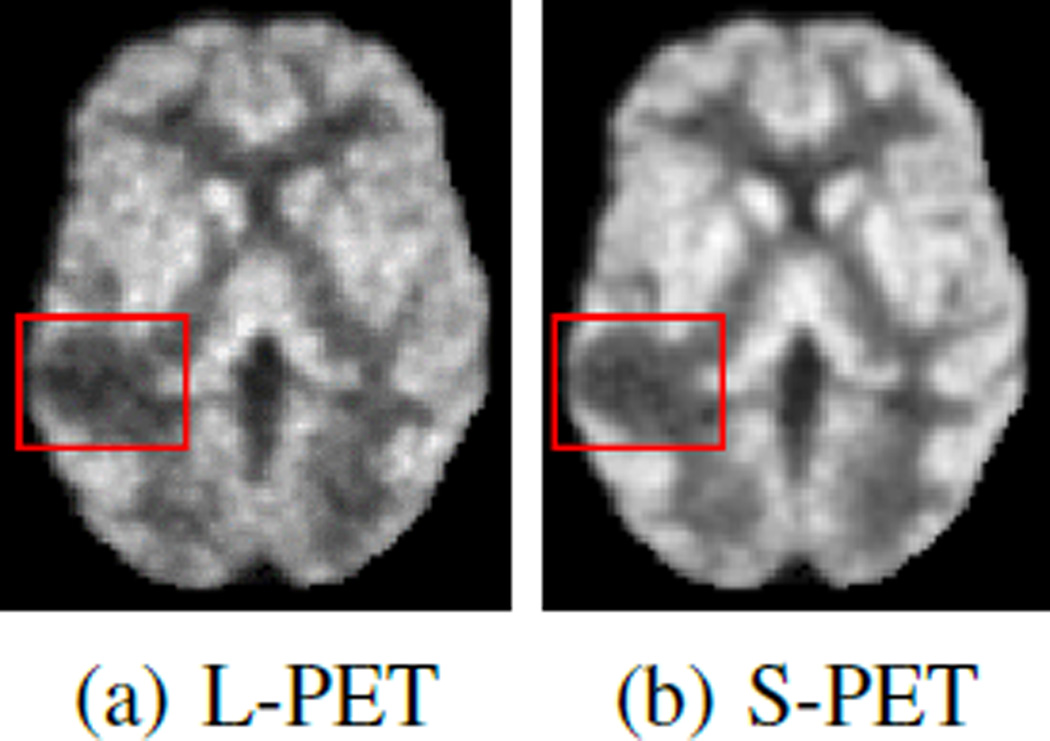
The phantom brain dataset is constructed from 20 anatomical normal brain models [33, 34]. Within each model, a 3-D “fuzzy” tissue membership volume is available for each tissue class, including background, cerebrospinal fluid, gray matter, white matter, fat, muscle, muscle/skin, skull, blood vessels, connective region around fat, dura matter and bone marrow. To examine the estimation quality especially in abnormal regions, we randomly place a lesion for each brain in the middle temporal gyrus. Fig. 4 shows examples of an L-PET image and the corresponding SPET image. Besides simulated PET images, each model has a T1-weighted MRI.
Fig. 4.
Sample images from brain phantom data. Bounding boxes enclose the lesion regions.
For the proof of concept, we want to answer the following questions:
Are the estimated S-PET alike images better than the original L-PET images?
Is performing the estimation in common space better than in the original image space?
Is multi-level CCA mapping more effective than a single-level CCA mapping?
Is MRI useful as additional estimation source?
Can comparable results be achieved by a denoising filter?
These questions are answered by evaluations using both image quality and clinical measures, as defined in the following.
2) Image Quality Evaluation
For quantitative evaluation, we first compute Peak Signal-to-Noise Ratio (PSNR) between an estimated S-PET image and the ground-truth S-PET image. PSNR is defined as
| (11) |
where DR denotes the dynamic range of the image, and the mean square error (MSE) between the estimation y and the ground-truth s with an image of size n × o × p is given by
| (12) |
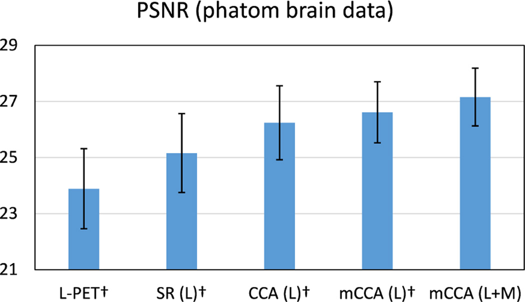
A larger value of PSNR indicates more similarities between the estimated S-PET image and the ground-truth S-PET images. Fig. 5 shows the average PSNR scores for the 20 subjects. Baseline comparisons include sparse representation in the original image space (SR), CCA, and multi-level CCA using L-PET as the only estimation source, while both multilevel CCA and multi-modal MRI are used in our method.
Fig. 5.
Average PSNR scores on the phantom brain dataset. Error bars indicate standard deviation. L means using L-PET as the only estimation source, and L+M means using both L-PET and MRI for estimation. Higher score is better. † indicates p < 0.01 in the t-test as compared to our method.
The results show that the estimation in the common space learned by CCA is more accurate than the estimation in the original image space. In addition, using more levels of common space learning leads to better results, which are further improved by leveraging MRI data. To validate the statistical significance of our method, we perform pairedsample t-test to compare the baseline methods against ours. As indicated in Fig. 5, p < 0.01 is observed for all the baseline methods under comparison. This provides further evidence about the advantage of our method, i.e., mCCA (L+M).
Furthermore, the Signal-to-Noise Ratio (SNR) is computed on the estimated images. SNR is defined as
| (13) |
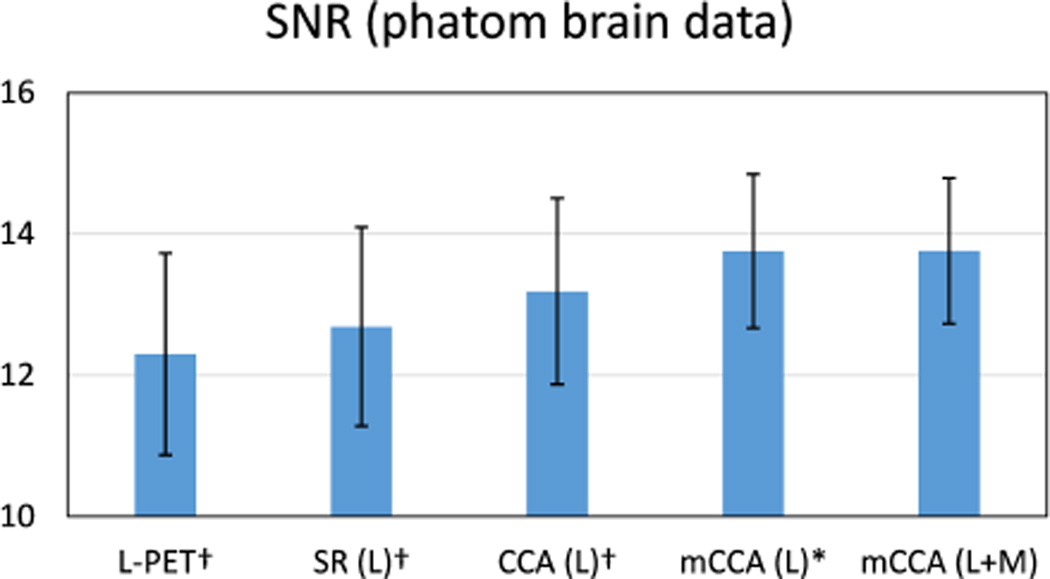
where mROI and σROI are the mean and standard deviation in the region of interest (ROI). In this case, the ROI is the lesion region. The average SNR values are shown in Fig. 6. Higher value of SNR indicates better quality. Compared to the other baseline methods, the highest SNR is achieved by the proposed method with statistical significance of p < 0. 05. The superior performance in SNR measure is congruent with the observation of the comparison of PSNR values.
Fig. 6.
Average SNR scores on the phantom brain dataset. The ROI for computing SNR is the lesion region. Error bars indicate standard deviation. L means using L-PET as the only estimation source, and L+M means using both L-PET and MRI for estimation. Higher score is better. † indicates p < 0.01 in the t-test as compared to our method, and * means p < 0.05.
3) Clinical Measure Evaluation
Besides image quality measure, it is also important that the ROI in an estimated S-PET image is well preserved in terms of clinical quantification, as compared to the ground-truth S-PET images. To examine this aspect, we evaluate two measures in the lesion region as the ROI. The first measure is Contrast-to-Noise Ratio (CNR), which is important in clinical applications to detect the potentially low remnant activity after therapy [14]. CNR is computed between ROI and the background (cerebellum in this paper). We use the definition of CNR in [35], i.e.,
| (14) |
where mROI and mBG are the mean intensities, σROI and σBG are the standard deviations of the ROI and the background, respectively.
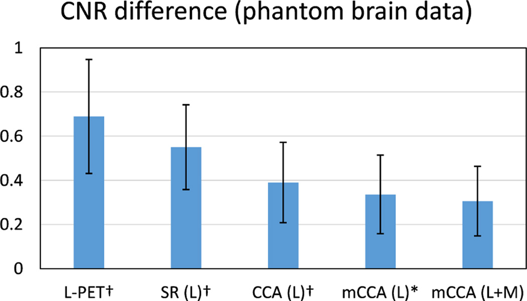
As the goal is to estimate S-PET images that are similar to the ground-truth S-PET images, we report the CNR difference between the estimated S-PET images and the ground-truth SPET images. Smaller difference indicates less deviation from the ground-truth. Fig. 7 shows the average CNR difference. We can see that the CNR difference is significant in the original L-PET images as well as the estimated S-PET images by patch-based SR. This difference is reduced by estimating the S-PET image in the common space learned by CCA, and the proposed mCCA scheme further bridges this difference. The small p-values, i.e., p < 0.05, demonstrate the statistical importance of the CNR results obtained by our method.
Fig. 7.
Average CNR difference on the phantom brain dataset. The ROI for computing CNR is the lesion region. L means using L-PET as the only estimation source, and L+M means using both L-PET and MRI for estimation. Error bars indicate standard deviation. Lower score is better. † indicates p < 0.01 in the t-test as compared to our method, and * means p < 0.05.
Apart from CNR, SUV calculated from the PET images is also critical for diagnostic evaluation and treatment planning [36]. The use of SUV can remove variability among patients, which is caused by the differences in body size and the amount of injected tracer dose. Particularly, the changes in SUV are important in clinical applications. For example, the SUV changes can be used to classify patients into different PET based treatment response categories, so such response classification can guide subsequent treatment decisions [37]. The SUV can be calculated on a per voxel basis, in which the value for a voxel at location (i,j,k) is defined by
| (15) |
where c(i,j,k) is the radioactivity concentration in that voxel (in kBq/ml) and w is the body weight of the subject (in g). a is the decay-corrected amount of injected dose (in kBq). As suggested in [13], smaller changes in SUV are highly desirable, meaning that the estimation does not significantly change the quantitative markers of the PET image. Thus, we report the SUV difference in the lesion region in both L-PET images and the estimated S-PET images, in order to examine how the SUV in these images deviates from the SUV in the ground-truth S-PET images.
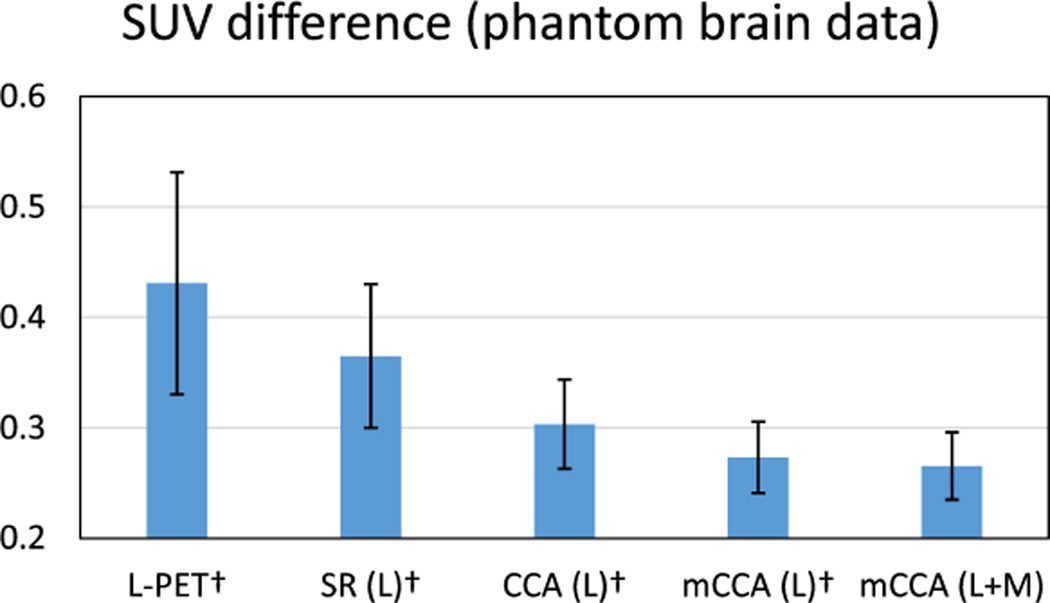
Fig. 8 shows the SUV difference in the same ROI by different methods. Compared to the baseline methods, the SUV difference by the proposed method is the smallest. This shows that the estimated S-PET images by our method can better preserve the SUV, indicating an improved clinical usability as compared to the L-PET images or the outputs by the baseline methods. This improvement is statistically important as suggested by the small p-values in comparison with other baseline methods.
Fig. 8.
Average SUV difference on the phantom brain dataset. The ROI for computing SUV is the lesion region. L means using L-PET as the only estimation source, and L+M means using both L-PET and MRI for estimation. Error bars indicate standard deviation. Lower score is better. † indicates p < 0.01 in the t-test as compared to our method.
Since image denoising can also improve the image quality, we compare our method with the following state-of-the-art denoising methods: 1) BM3D [38], which is a denoising method based on an enhanced sparse representation in transform-domain, and it has also shown favorable performance in PET sinogram denoising [39]; 2) Optimized Blockwise Nonlocal Means (OBNM) [40], which is originally developed for 3D MR images and can also be applied to PET images. The denoising directly operates on the L-PET input. The comparison results, in terms of different measures, are listed in Table I. Note that, for fair comparison, only L-PET is used as the estimation source in our method in this comparison.
TABLE I.
Comparison with different denoising methods. For PSNR and SNR, higher score is better. For CNR and SUV difference, lower score is better.
| Method | PSNR | SNR | CNR diff. | SUV diff. |
|---|---|---|---|---|
| mCCA | 26.61 ± 1.31 | 13.75 ± 0.91 | 0.33 ± 0.18 | 0.27 ± 0.03 |
| BM3D [38] | 24.21 ± 1.94† | 13.17 ± 0.97† | 0.72 ± 0.48† | 0.39 ± 0.10† |
| OBNM [40] | 24.49 ± 1.86† | 13.22 ± 0.96† | 0.45 ± 0.20† | 0.37 ± 0.07† |
indicates p < 0.01 in the t-test as compared to our method.
We observe from the results in Table I that our estimated S-PET images are notably better than the denoised L-PET images. In other words, a simple denoising process cannot produce S-PET alike images that are close to the groundtruth S-PET images, and the clinical quantification cannot be well preserved. To verify the statistical significance, we also perform t-test to compare the results by the two denoising methods against the proposed method, and in all different measures, a small p-value, i.e., p < 0.01, is observed.
The evaluations on the phantom brain dataset with abnormal structures (i.e., lesion), using both image quality and clinical quantification measures, with comparisons to baseline methods, suggest that: 1) the estimated S-PET images are more similar to the ground-truth S-PET images, compared to the L-PET images and outputs by other baseline methods, 2) estimation in common space is more effective than that in the original image space, 3) multi-level CCA common space learning leads to improved results, 4) MRI can help further improve the estimation accuracy, and 5) performing simple denoising is not adequate to produce S-PET alike images that are close to the ground-truth S-PET images.
B. Real Brain Dataset
1) Data Description
We further evaluate the performance of our method on a real brain dataset. This dataset consists of PET and MR brain images from 11 subjects (6 females and 5 males). Based on clinical examination, all subjects were encouraged to have PET scans. Table II summarizes their demographic information. Among these subjects, subject 9-11 were diagnosed with Mild Cognitive Impairment (MCI). All scans were acquired on a Siemens Biograph mMR MR-PET system. This study was approved by the University of North Carolina at Chapel Hill Institutional Review Board.
TABLE II.
Demographic information of the subjects in the experiments
| Subject ID | Age | Gender (F, M) | Weight (Kg) |
|---|---|---|---|
| 1 | 26 | F | 50.3 |
| 2 | 30 | M | 137.9 |
| 3 | 33 | M | 103.0 |
| 4 | 25 | F | 85.7 |
| 5 | 18 | F | 59.9 |
| 6 | 19 | M | 72.6 |
| 7 | 36 | M | 102.1 |
| 8 | 28 | F | 83.9 |
| 9 | 65 | M | 68.0 |
| 10 | 86 | F | 68.9 |
| 11 | 86 | M | 74.8 |
The standard-dose and low-dose correspond to standard activity administered (averaging 203 MBq and effective dose of 3.86 mSv) and low activity administered (approximately 51 MBq and effective dose of 0.97 mSv), respectively. In general, the effective dose can be regarded as proportional to the administered activity [41]. In our case, the standard-dose activity level is at the low end of the recommended range (185 to 740 MBq) by the Society of Nuclear Medicine and Molecular Imaging (SNMMI) [41]. During PET scanning, the standard-dose scan was performed for a full 12 minutes within 60 minutes of injection of 18F-FDG radioactive tracer, based on standard protocols. A second PET scan was acquired immediately after the first scan in list-mode for 12 minutes. The second scan was then broken up into four separate 3-minute sets, each of which is considered as a low-dose scan. As a result, the activity level in the 3-minute scan is significantly lower than the recommended range.
In other words, the L-PET images are completely separate from the S-PET images in the acquisition process in this setting. On the contrary, if only the first scan was obtained and the low-dose scans were acquired by breaking the first scan into four sets, the L-PET images and the S-PET images would actually come from the same set of data, despite of the dose difference. It is worthwhile to note that reducing acquisition time at standard-dose is considered as a surrogate for standard acquisition time at a reduced dose. Regarding reconstruction, all PET scans were reconstructed using standard methods from the vendor. Attenuation correction using the Dixon sequence and corrections for scatters were applied to PET images. The reconstruction was performed iteratively using the OS-EM algorithm [42] with three iterations, 21 subsets, and post-reconstruction filtered with a 3D Gaussian with sigma of 2 mm. Each PET image has a voxel size of 2.09 × 2.09 × 2.03mm3.
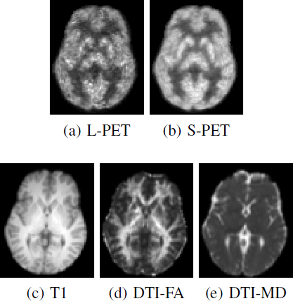
Besides PET images, structural MR images were acquired with a 1 × 1 × 1mm3 resolution, and diffusion images were also acquired with a resolution of 2 × 2 × 2mm3. Then we compute FA and MD images from the diffusion images. For each subject, the MR images were linearly aligned to the corresponding PET image, and then all of the images were aligned to the first subject using FLIRT [43]. Non-brain tissues were then removed from the aligned images using a skull stripping method [44]. In summary, each subject has an L-PET image, an S-PET image, and three MR images (T1-weighted MRI, FA and MD). Fig. 9 shows examples of PET and MR images from one subject.
Fig. 9.
Sample PET and MR images of one subject from real brain data.
2) Image Quality Evaluation
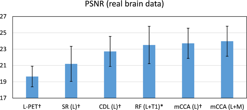
For comparison, the bench-mark methods include SR, coupled dictionary learning (CDL) [20], regression forest (RF) [18]. Fig. 10 shows the PSNR results. We note that by using L-PET as the only estimation source, the proposed method achieves the highest PSNR scores. With additional MRI data, further improvement is obtained with a PSNR of 23.9 by our method. In addition, the small p-values from the t-test verify the statistical significance of our method.
Fig. 10.
Average PSNR on the real brain dataset. L means using L-PET as the only estimation source, and L+M means using both L-PET and MRI for estimation. Error bars indicate standard deviation. Number below each method name is the max deviation. † indicates p < 0.01 in the t-test as compared to our method, and * means p < 0.05.
To more thoroughly examine the performance of our method, for each subject, eight ROIs were segmented based on the T1-weighted MR image, and the estimation performance within each ROI is evaluated separately. Specifically, on each hemisphere of the brain (i.e., left or right), four ROIs, including frontal lobe, parietal lobe, occipital lobe, and temporal lobe, were separated. We use Automated Anatomical Labeling (AAL) template [45] and merge related regions to cover these ROIs. Table III shows the SNR results for each ROI. Higher value of SNR indicates better quality. Compared to other methods, the highest SNR is achieved by the proposed multilevel CCA with all estimation sources. This observation is unanimous for all ROIs. The t-test also yields p-values lower than 0.05 when comparing our method with the others.
TABLE III.
Signal-to-Noise Ratio (SNR) in different ROIs on the real brain dataset. Higher score is better. SD is standard deviation and MD is max deviation.
| ROI | L-PET | SR | CDL | RF | mCCA | mCCA |
|---|---|---|---|---|---|---|
| L | L | L+T1 | L | L+M | ||
| 1 | 7.53 | 8.23 | 8.56 | 8.73 | 8.72 | 8.76 |
| 2 | 8.30 | 8.89 | 9.07 | 9.15 | 9.42 | 9.51 |
| 3 | 7.98 | 7.99 | 8.64 | 9.01 | 9.24 | 9.40 |
| 4 | 8.34 | 7.71 | 8.34 | 7.10 | 9.45 | 9.64 |
| 5 | 10.25 | 10.50 | 10.93 | 11.58 | 12.19 | 12.41 |
| 6 | 10.61 | 10.32 | 11.02 | 10.36 | 12.35 | 12.62 |
| 7 | 11.09 | 11.22 | 12.95 | 12.57 | 13.02 | 13.31 |
| 8 | 11.66 | 11.91 | 13.35 | 13.21 | 13.66 | 13.96 |
| Average | 9.5† | 9.6† | 10.4† | 11.1* | 11.0† | 11.2 |
| SD | 1.60 | 1.60 | 2.01 | 2.10 | 1.99 | 2.07 |
| MD | 2.19 | 2.31 | 2.99 | 3.00 | 2.65 | 2.76 |
indicates p < 0.01 in the t-test as compared to our method, and
means p < 0.05.
3) Clinical Measure Evaluation
We further evaluate the proposed method in terms of clinical usability. Specifically, CNR is first calculated in each of the eight ROIs, and the cerebellum is used as the background region. The CNR difference, which measures how close the CNR in our estimated S-PET images deviates from that in the ground-truth, is reported in Table V.
TABLE V.
Standard Uptake Value (SUV) difference for the MCI subjects. Lower score is better. SD is standard deviation and MD is max deviation.
| Subject | L-PET | SR | CDL | RF | mCCA | mCCA |
|---|---|---|---|---|---|---|
| L | L | L+T1 | L | L+M | ||
| 9 | 0.646 | 0.094 | 0.017 | 0.334 | 0.010 | 0.006 |
| 10 | 1.612 | 0.275 | 0.238 | 0.823 | 0.182 | 0.169 |
| 11 | 0.637 | 0.104 | 0.050 | 0.155 | 0.011 | 0.001 |
| Average | 0.965 | 0.158 | 0.101 | 0.437 | 0.068 | 0.059 |
| SD | 0.560 | 0.102 | 0.119 | 0.346 | 0.099 | 0.095 |
| MD | 0.647 | 0.117 | 0.136 | 0.358 | 0.115 | 0.110 |
Compared to the other methods, the CNR difference by the proposed method is the smallest for different ROIs. Also, the superior performance is further corroborated by the p-values which are all smaller than 0.05. This shows that the estimated S-PET images by our method are most similar to the groundtruth S-PET images, indicating an improved clinical usability as compared to the L-PET images or the outputs by the other methods.
Furthermore, since three subjects in this dataset (Subject 9–11) are diagnosed with MCI, it is particularly important that the estimated S-PET images by our method can well preserve the SUV in the hippocampal regions. Therefore, we calculate the SUV difference on these regions for the MCI subjects. The results are listed in Table V. As observed, the SUV is well maintained by our method with minimum deviation from the true SUV in the ground-truth S-PET images. This suggest that not only our method can well preserve the measures in the normal brain parts, but also in abnormal regions the clinical quantification is well retained.
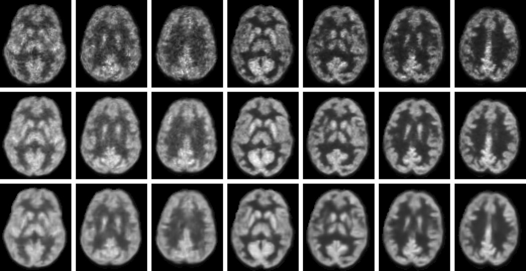
For qualitative results, some samples of the estimated S-PET images by our method are shown in Fig. 11. For comparison, the corresponding L-PET images and the ground-truth S-PET images are also provided. As observed, the estimated S-PET images are very close to the ground-truth. Compared to the L-PET images, better visual quality is observed in both the ground-truth S-PET images and the estimated S-PET images. The estimated images are smoother than the ground-truth due to the averaging of patches in the final construction of the output images. This process also helps reduce noise level as evidenced by the improved SNR in Table III. In summary, both quantitative and visual results suggest that the S-PET images can be well estimated by our method, in terms of image quality and clinical quantification measures that are critical in diagnosis.
Fig. 11.
Visual comparisons of L-PET images (top), ground-truth S-PET images (middle), and the estimated S-PET images by our method (bottom).
C. Computational Cost
We implemented our algorithm in Matlab on a PC with Intel 2.4GHz CPU and 8GB memory. The main computation is on the LLC part as in Eq. (5), with the complexity of O(K2), where K is the dictionary size. Regarding the computational cost, it takes about 120 seconds to estimate one slice of a 3D PET image in our data. Since our approach is data-driven, meaning that at each voxel location, training patches have to be selected and mappings have to be learned. Therefore, computation is not quite efficient in our current implementation. However, further speedup of our method is possible. For example, the estimation of each slice can be performed independently, thus a parallel computing scheme for each slice can significantly improve the efficiency.
D. Discussion
The evaluation performed here compares S-PET to L-PET in the context of using the same PET-MR scanner for the same acquisition time. This approach makes the comparison fair and leaves other variables out of the analysis. Nevertheless, other approaches to improve PET image quality under low-dose conditions also exist, including increasing the scan time or taking advantage of other features, such as time-of-flight, although it is currently not available on the Biograph mMR. It is recommended that future studies will consider these other methods along with our technique in determining the best approach for a specific clinical or research protocol.
The proposed method can be generalized to other PET targets, applications, and scanning protocols; but, in order to maintain a controlled experiment, we did the evaluation in the context of FDG brain PET with a specific dose reduction on the same scanner controlled for the same scan time. Thus, the conclusions regarding performance should be limited at this time to these specific conditions. Future studies will consider how performance changes under different dose-reduction ratios, with different PET tracers, and in different anatomical targets.
Regarding the radiation, although a single PET scan has low radiation, multiple scans may accumulate the radiation. Based on the report from Biological Effects of Ionizing Radiation (BEIR VII)1, the increased risk of incidence of cancer is 10.8% per Sv. In other words, one brain PET scan increases the risk of lifetime cancer by 0.04%. The International Commission on Radiation Protection considers the increased risk of death by cancer to be about 4% per Sv, meaning that one brain PET scan increases the risk of death from cancer by 0.015%. Although these numbers are small, but the risks are accumulated for patients who undergo multiple PET scans as part of their treatment plan. In addition, pediatric patients have increased risks. Therefore, the long-term focus of this work is to reduce the total dose for the non-standard population with increased risk from PET radiation.
IV. Conclusions
A multi-level CCA scheme has been proposed for estimating S-PET images from L-PET and multi-modal MR images. On both phantom and real brain datasets, extensive evaluations using both image quality and clinical measures have demonstrated the effectiveness of the proposed method. Notably, in the estimated S-PET images, the desired quantification measures such as SUV were faithfully preserved as compared to the ground-truth S-PET images. As compared to other rival methods, our approach achieved superior performance.
In this work, we have demonstrated that high quality SPET alike images can be estimated offline in a learning based framework from low-dose PET and MR images. This potentially meets an important clinical demand to significantly reduce the radioactive tracer injection during PET scanning. In the future, more effective estimation and fusion techniques will be studied to improve the estimation quality.
We have drawn our conclusions based on quantitative measures on two datasets. In future, we plan to enroll more subjects in our dataset to more rigorously evaluate the proposed method. To further validate the effectiveness of our method in clinical tasks, larger scale experiments and evaluations by physicians should be conducted, which is our ongoing work.
TABLE IV.
Contrast-to-Noise Ratio (CNR) difference in different ROIs on the real brain dataset. Lower score is better. SD is standard deviation and MD is max deviation.
| ROI | L-PET | SR | CDL | RF | mCCA | mCCA |
|---|---|---|---|---|---|---|
| L | L | L+T1 | L | L+M | ||
| 1 | 0.148 | 0.192 | 0.095 | 0.027 | 0.016 | 0.013 |
| 2 | 0.121 | 0.183 | 0.103 | 0.034 | 0.018 | 0.015 |
| 3 | 0.172 | 0.184 | 0.085 | 0.052 | 0.021 | 0.017 |
| 4 | 0.151 | 0.167 | 0.114 | 0.076 | 0.003 | 0.001 |
| 5 | 0.074 | 0.027 | 0.023 | 0.017 | 0.018 | 0.016 |
| 6 | 0.042 | 0.035 | 0.029 | 0.019 | 0.013 | 0.012 |
| 7 | 0.251 | 0.072 | 0.066 | 0.071 | 0.028 | 0.024 |
| 8 | 0.273 | 0.081 | 0.059 | 0.047 | 0.024 | 0.021 |
| Average | 0.154† | 0.118† | 0.071† | 0.043* | 0.018† | 0.015 |
| SD | 0.071 | 0.079 | 0.034 | 0.023 | 0.008 | 0.007 |
| MD | 0.119 | 0.091 | 0.049 | 0.033 | 0.015 | 0.014 |
indicates p < 0.01 in the t-test as compared to our method, and
means p < 0.05.
Acknowledgments
This work was supported by NIH grants (EB006733, EB008374, EB009634, MH100217, AG041721, AG049371, AG042599).
Biographies

Le An received the B.Eng. degree in telecommunications engineering from Zhejiang University in China in 2006, the M.Sc. degree in electrical engineering from Eindhoven University of Technology in Netherlands in 2008, and the Ph.D. degree in electrical engineering from University of California, Riverside in USA in 2014. His research interests include image processing, computer vision, pattern recognition, and machine learning.

Pei Zhang received his Ph.D. at the University of Manchester in 2011. He then took up a research position at the University of North Carolina at Chapel Hill. His major interests involve computer vision, machine learning and their applications in medical image analysis. He has published 10+ peer-reviewed papers in major international journals and conferences.

Ehsan Adeli received his Ph.D. from Iran University of Science and Technology. He is now working as a post-doctoral research fellow at the Biomedical Research Imaging Center, University of North Carolina at Chapel Hill. He has previously worked as a visiting research scholar at the Robotics Institute, Carnegie Mellon University in Pittsburgh, PA. Dr. Adeli’s research interests include machine learning, computer vision, multimedia and image processing with applications on medical imaging.

Yan Wang received her Bachelor, Master and Doctor’s degree in College of Electronic and Information Engineering of Sichuan University in China in 2009, 2012 and 2015, respectively. She joined the College of Computer Science of Sichuan University as an assistant professor. She was a visiting scholar with the Department of Radiology, University of North Carolina at Chapel Hill from 2014 to 2015. Her research interests focus on the inverse problems in imaging science, including image denoising, segmentation, inpainting, and medical image reconstruction, etc.

Guangkai Ma received the B.S. degree from Harbin University Of Science And Technology, China in 2010; the M.E. degree from Harbin Institute of Technology, China in 2012. He was a joint Ph.D. student in the Department of Radiology and BRIC, University of North Carolina at Chapel Hill, NC, USA from 2013 to 2015. He is currently pursuing his Ph.D. degree in Inertial Technology Research Center, Harbin Institute of Technology, China. His current research interests include gait recognition, pattern recognition and medical image segmentation.

Feng Shi is currently an assistant professor in Department of Radiology at the University of North Carolina at Chapel Hill. He has studied Computer Science at the Institute of Automation, Chinese Academy of Sciences and received his PhD degree in 2008. His research interests include machine learning, neuro and cardiac imaging, multimodal image analysis, and computer-aided early diagnosis.

David S. Lalush is with the North Carolina State University and The University of North Carolina at Chapel Hill Joint Department of Biomedical Engineering. His current research interests include simultaneous PET-MRI image processing, analysis, and clinical applications, as well as X-ray imaging, tomographic reconstruction, and general image and signal processing.

Weili Lin is the director of the Biomedical Research Imaging Center (BRIC), Dixie Lee Boney Soo Distinguished Professor of Neurological Medicine, and the vice chair of the Department of Radiology at the University of North Carolina at Chapel Hill. His research interests include cerebral ischemia, human brain development, PET, and MR.

Dinggang Shen is a Professor of Radiology, Biomedical Research Imaging Center (BRIC), Computer Science, and Biomedical Engineering in the University of North Carolina at Chapel Hill (UNCCH). He is currently directing the Center for Image Analysis and Informatics, the Image Display, Enhancement, and Analysis (IDEA) Lab in the Department of Radiology, and also the medical image analysis core in the BRIC. He was a tenure-track assistant professor in the University of Pennsylvanian (UPenn), and a faculty member in the Johns Hopkins University. Dr. Shen’s research interests include medical image analysis, computer vision, and pattern recognition. He has published more than 700 papers in the international journals and conference proceedings. He serves as an editorial board member for six international journals. He also served in the Board of Directors, The Medical Image Computing and Computer Assisted Intervention (MICCAI) Society, in 2012–2015.
Footnotes
Contributor Information
Le An, Department of Radiology and Biomedical Research Imaging Center, University of North Carolina at Chapel Hill, Chapel Hill 27599, USA.
Pei Zhang, Department of Radiology and Biomedical Research Imaging Center, University of North Carolina at Chapel Hill, Chapel Hill 27599, USA.
Ehsan Adeli, Department of Radiology and Biomedical Research Imaging Center, University of North Carolina at Chapel Hill, Chapel Hill 27599, USA.
Yan Wang, College of Computer Science, Sichuan University, Chengdu 610064, China.
Guangkai Ma, Department of Radiology and Biomedical Research Imaging Center, University of North Carolina at Chapel Hill, Chapel Hill 27599, USA.
Feng Shi, Department of Radiology and Biomedical Research Imaging Center, University of North Carolina at Chapel Hill, Chapel Hill 27599, USA.
David S. Lalush, Joint UNC-NCSU Department of Biomedical Engineering, North Carolina State University, Raleigh, NC 27695, USA.
Weili Lin, MRI Lab, Department of Radiology and BRIC, University of North Carolina at Chapel Hill, Chapel Hill 27599, USA.
Dinggang Shen, Department of Radiology and Biomedical Research Imaging Center, University of North Carolina at Chapel Hill, Chapel Hill 27599, USA. He is also with the Department of Brain and Cognitive Engineering, Korea University, Seoul 02841, Republic of Korea.
References
- 1.Chen W. Clinical applications of PET in brain tumors. Journal of Nuclear Medicine. 2007;48(9):1468–1481. doi: 10.2967/jnumed.106.037689. [DOI] [PubMed] [Google Scholar]
- 2.Quigley H, Colloby SJ, O’Brien JT. PET imaging of brain amyloid in dementia: A review. International Journal of Geriatric Psychiatry. 2011;26(10):991–999. doi: 10.1002/gps.2640. [DOI] [PubMed] [Google Scholar]
- 3.Alessio A, Vesselle H, Lewis D, Matesan M, Behnia F, Suhy J, de Boer B, Maniawski P, Minoshima S. Feasibility of low-dose FDG for whole-body TOF PET/CT oncologic workup. Journal of Nuclear Medicine (abstract) 2012;53:476. [Google Scholar]
- 4.Pichler BJ, Kolb A, Nägele T, H-P Schlemmer. PET/MRI: Paving the way for the next generation of clinical multimodality imaging applications. Journal of Nuclear Medicine. 2010;51(3):333–336. doi: 10.2967/jnumed.109.061853. [DOI] [PubMed] [Google Scholar]
- 5.Vunckx K, Atre A, Baete K, Reilhac A, Deroose C, Van Laere K, Nuyts J. Evaluation of three MRI-based anatomical priors for quantitative PET brain imaging. IEEE Transactions on Medical Imaging. 2012 Mar;31(3):599–612. doi: 10.1109/TMI.2011.2173766. [DOI] [PubMed] [Google Scholar]
- 6.Ehrhardt MJ, Thielemans K, Pizarro L, Atkinson D, Ourselin S, Hutton BF, Arridge SR. Joint reconstruction of PET-MRI by exploiting structural similarity. Inverse Problems. 2015;31(1):015001. [Google Scholar]
- 7.Tang J, Rahmim A. Anatomy assisted PET image reconstruction incorporating multi-resolution joint entropy. Physics in Medicine and Biology. 2015;60(1):31–48. doi: 10.1088/0031-9155/60/1/31. [DOI] [PMC free article] [PubMed] [Google Scholar]
- 8.Nguyen V-G, Lee S-J. Incorporating anatomical side information into PET reconstruction using nonlocal regularization. IEEE Transactions on Image Processing. 2013;22(10):3961–3973. doi: 10.1109/TIP.2013.2265881. [DOI] [PubMed] [Google Scholar]
- 9.Chan C, Fulton R, Barnett R, Feng D, Meikle S. Postreconstruction nonlocal means filtering of whole-body PET with an anatomical prior. IEEE Transactions on Medical Imaging. 2014 Mar;33(3):636–650. doi: 10.1109/TMI.2013.2292881. [DOI] [PubMed] [Google Scholar]
- 10.Chun SY, Fessler JA, Dewaraja YK. Post-reconstruction nonlocal means filtering methods using CT side information for quantitative SPECT. Physics in Medicine and Biology. 2013;58(17):6225–6240. doi: 10.1088/0031-9155/58/17/6225. [DOI] [PMC free article] [PubMed] [Google Scholar]
- 11.Yan J, Lim JC-S, Townsend DW. MRI-guided brain PET image filtering and partial volume correction. Physics in Medicine and Biology. 2015;60(3):961–976. doi: 10.1088/0031-9155/60/3/961. [DOI] [PubMed] [Google Scholar]
- 12.Turkheimer FE, Boussion N, Anderson AN, Pavese N, Piccini P, Visvikis D. PET image denoising using a synergistic multiresolution analysis of structural (MRI/CT) and functional datasets. Journal of Nuclear Medicine. 2008;49(4):657–666. doi: 10.2967/jnumed.107.041871. [DOI] [PubMed] [Google Scholar]
- 13.Bagci U, Mollura D. Denoising PET images using singular value thresholding and Stein’s unbiased risk estimate. Medical Image Computing and Computer-Assisted Intervention (MICCAI) 2013:115–122. doi: 10.1007/978-3-642-40760-4_15. [DOI] [PMC free article] [PubMed] [Google Scholar]
- 14.Dutta J, Leahy RM, Li Q. Non-local means denoising of dynamic PET images. PLoS ONE. 2013;8(12):e81390. doi: 10.1371/journal.pone.0081390. [DOI] [PMC free article] [PubMed] [Google Scholar]
- 15.Pogam AL, Hanzouli H, Hatt M, Rest CCL, Visvikis D. Denoising of PET images by combining wavelets and curvelets for improved preservation of resolution and quantitation. Medical Image Analysis. 2013;17(8):877–891. doi: 10.1016/j.media.2013.05.005. [DOI] [PubMed] [Google Scholar]
- 16.Xu Z, Bagci U, Gao M, Mollura DJ. Highly precise partial volume correction for PET images: An iterative approach via shape consistency; 12th IEEE International Symposium on Biomedical Imaging (ISBI); 2015. Apr, pp. 1196–1199. [Google Scholar]
- 17.Kang J, Gao Y, Wu Y, Ma G, Shi F, Lin W, Shen D. Prediction of standard-dose PET image by low-dose PET and MRI images. Machine Learning in Medical Imaging. 2014:280–288. [Google Scholar]
- 18.Kang J, Gao Y, Shi F, Lalush DS, Lin W, Shen D. Prediction of standard-dose brain PET image by using MRI and low-dose brain [18F]FDG PET images. Medical Physics. 2015;42(9):5301–5309. doi: 10.1118/1.4928400. [DOI] [PMC free article] [PubMed] [Google Scholar]
- 19.Fang R, Zhang S, Chen T, Sanelli P. Robust low-dose CT perfusion deconvolution via tensor total-variation regularization. IEEE Transactions on Medical Imaging. 2015 Jul;34(7):1533–1548. doi: 10.1109/TMI.2015.2405015. [DOI] [PMC free article] [PubMed] [Google Scholar]
- 20.Wang B, Li L. Recent development of dual-dictionary learning approach in medical image analysis and reconstruction. Computational and Mathematical Methods in Medicine. 2015;2015:1–9. doi: 10.1155/2015/152693. [DOI] [PMC free article] [PubMed] [Google Scholar]
- 21.Hotelling H. Relations between two sets of variates. Biometrika. 1936;28(3/4):321–377. [Google Scholar]
- 22.Lee G, Singanamalli A, Wang H, Feldman M, Master S, Shih N, Spangler E, Rebbeck T, Tomaszewski J, Madabhushi A. Supervised multi-view canonical correlation analysis (sMVCCA): Integrating histologic and proteomic features for predicting recurrent prostate cancer. IEEE Transactions on Medical Imaging. 2015 Jan;34(1):284–297. doi: 10.1109/TMI.2014.2355175. [DOI] [PubMed] [Google Scholar]
- 23.Zhu X, Suk H-I, Shen D. Multi-modality canonical feature selection for Alzheimer’s disease diagnosis. Medical Image Computing and Computer-Assisted Intervention (MICCAI) 2014:162–169. doi: 10.1007/978-3-319-10470-6_21. [DOI] [PMC free article] [PubMed] [Google Scholar]
- 24.Dhillon P, Avants B, Ungar L, Gee J. Partial sparse canonical correlation analysis (PSCCA) for population studies in medical imaging; 9th IEEE International Symposium on Biomedical Imaging (ISBI); 2012. May, pp. 1132–1135. [Google Scholar]
- 25.Heinrich M, Papież B, Schnabel J, Handels H. Multispectral image registration based on local canonical correlation analysis. Medical Image Computing and Computer-Assisted Intervention (MICCAI) 2014:202–209. doi: 10.1007/978-3-319-10404-1_26. [DOI] [PubMed] [Google Scholar]
- 26.Correa N, Adali T, Li Y-O, Calhoun V. Canonical correlation analysis for data fusion and group inferences. IEEE Signal Processing Magazine. 2010;27(4):39–50. doi: 10.1109/MSP.2010.936725. [DOI] [PMC free article] [PubMed] [Google Scholar]
- 27.Krol A, Naveed M, McGrath M, Lisi M, Lavalley C, Feiglin D. Very low-dose adult whole-body tumor imaging with F-18 FDG PET/CT. Medical Imaging 2015: Biomedical Applications in Molecular, Structural, and Functional Imaging. 2015:941 711–1–941 711–6. [Google Scholar]
- 28.Wang Z, Bovik A, Sheikh H, Simoncelli E. Image quality assessment: from error visibility to structural similarity. IEEE Transactions on Image Processing. 2004;13(4):600–612. doi: 10.1109/tip.2003.819861. [DOI] [PubMed] [Google Scholar]
- 29.Coupé P, Manjón JV, Fonov V, Pruessner J, Robles M, Collins DL. Patch-based segmentation using expert priors: Application to hippocampus and ventricle segmentation. NeuroImage. 2011;54(2):940–954. doi: 10.1016/j.neuroimage.2010.09.018. [DOI] [PubMed] [Google Scholar]
- 30.Wang J, Yang J, Yu K, Lv F, Huang T, Gong Y. Locality-constrained linear coding for image classification; IEEE Conference on Computer Vision and Pattern Recognition (CVPR); 2010. pp. 3360–3367. [Google Scholar]
- 31.Yu K, Zhang T, Gong Y. Nonlinear learning using local coordinate coding. Advances in Neural Information Processing Systems. 2009:2223–2231. [Google Scholar]
- 32.Chen Y, Mairal J, Harchaoui Z. Fast and robust archetypal analysis for representation learning; IEEE Conference on Computer Vision and Pattern Recognition (CVPR); 2014. pp. 1478–1485. [Google Scholar]
- 33.Aubert-Broche B, Griffin M, Pike G, Evans A, Collins D. Twenty new digital brain phantoms for creation of validation image data bases. IEEE Trans. on Med.l Imag. 2006 Nov;25(11):1410–1416. doi: 10.1109/TMI.2006.883453. [DOI] [PubMed] [Google Scholar]
- 34.Aubert-Broche B, Evans AC, Collins L. A new improved version of the realistic digital brain phantom. Neuroimage. 2006;32(1):138–145. doi: 10.1016/j.neuroimage.2006.03.052. [DOI] [PubMed] [Google Scholar]
- 35.Lartizien C, Kinahan PE, Comtat C. A lesion detection observer study comparing 2-dimensional versus fully 3-dimensional whole-body PET imaging protocols. Journal of Nuclear Medicine. 2004;45(4):714–723. [PubMed] [Google Scholar]
- 36.Kinahan PE, Fletcher JW. Positron emission tomography-computed tomography standardized uptake values in clinical practice and assessing response to therapy. Seminars in Ultrasound, CT and MRI. 2010;31(6):496–505. doi: 10.1053/j.sult.2010.10.001. [DOI] [PMC free article] [PubMed] [Google Scholar]
- 37.Vanderhoek M, Perlman SB, Jeraj R. Impact of different standardized uptake value measures on PET-based quantification of treatment response. Journal of Nuclear Medicine. 2013;54(8):1188–1194. doi: 10.2967/jnumed.112.113332. [DOI] [PMC free article] [PubMed] [Google Scholar]
- 38.Dabov K, Foi A, Katkovnik V, Egiazarian K. Image denoising by sparse 3-D transform-domain collaborative filtering. IEEE Transactions on Image Processing. 2007 Aug;16(8):2080–2095. doi: 10.1109/tip.2007.901238. [DOI] [PubMed] [Google Scholar]
- 39.Peltonen S, Tuna U, Ruotsalainen U. Low count PET sinogram denoising; IEEE Nuclear Science Symposium and Medical Imaging Conference (NSS/MIC); 2012. Oct, pp. 3964–3967. [Google Scholar]
- 40.Coupé P, Yger P, Prima S, Hellier P, Kervrann C, Barillot C. An optimized blockwise nonlocal means denoising filter for 3-D magnetic resonance images. IEEE Transactions on Medical Imaging. 2008 Apr;27(4):425–441. doi: 10.1109/TMI.2007.906087. [DOI] [PMC free article] [PubMed] [Google Scholar]
- 41.Waxman AD, Herholz K, Lewis DH, Herscovitch P, Minoshima S, Ichise M, Drzezga AE, Devous MD, Mountz JM. Society of nuclear medicine procedure guideline for FDG PET brain imaging. Society of Nuclear Medicine. 2009:1–12. version 1.0. [Google Scholar]
- 42.Hudson H, Larkin R. Accelerated image reconstruction using ordered subsets of projection data. IEEE Transactions on Medical Imaging. 1994 Dec;13(4):601–609. doi: 10.1109/42.363108. [DOI] [PubMed] [Google Scholar]
- 43.Fischer B, Modersitzki J. FLIRT: A flexible image registration toolbox. Biomedical Image Registration. 2003;2717:261–270. [Google Scholar]
- 44.Shi F, Wang L, Dai Y, Gilmore JH, Lin W, Shen D. LABEL: Pediatric brain extraction using learning-based meta-algorithm. NeuroImage. 2012;62(3):1975–1986. doi: 10.1016/j.neuroimage.2012.05.042. [DOI] [PMC free article] [PubMed] [Google Scholar]
- 45.Tzourio-Mazoyer N, Landeau B, Papathanassiou D, Crivello F, Etard O, Delcroix N, Mazoyer B, Joliot M. Automated anatomical labeling of activations in SPM using a macroscopic anatomical parcellation of the MNI MRI single-subject brain. NeuroImage. 2002;15(1):273–289. doi: 10.1006/nimg.2001.0978. [DOI] [PubMed] [Google Scholar]


