A Robust Parameterization of Human Gait Patterns Across Phase-Shifting Perturbations

Abstract

The phase of human gait is difficult to quantify accurately in the presence of disturbances. In contrast, recent bipedal robots use time-independent controllers relying on a mechanical phase variable to synchronize joint patterns through the gait cycle. This concept has inspired studies to determine if human joint patterns can also be parameterized by a mechanical variable. Although many phase variable candidates have been proposed, it remains unclear which, if any, provide a robust representation of phase for human gait analysis or control. In this paper we analytically derive an ideal phase variable (the hip phase angle) that is provably monotonic and bounded throughout the gait cycle. To examine the robustness of this phase variable, ten able-bodied human subjects walked over a platform that randomly applied phase-shifting perturbations to the stance leg. A statistical analysis found the correlations between nominal and perturbed joint trajectories to be significantly greater when parameterized by the hip phase angle (0.95+) than by time or a different phase variable. The hip phase angle also best parameterized the transient errors about the nominal periodic orbit. Finally, interlimb phasing was best explained by local (ipsilateral) hip phase angles that are synchronized during the double-support period.

I. Introduction

The current methodology used to study the human gait cycle as a periodic process consisting of discrete events (e.g., heel strike, load acceptance, toe off, pre-swing, mid-swing, etc. [1], [2]) has greatly influenced the approaches taken to control prosthetic legs and exoskeletons [3]–[5]. Even though this convention has given us vast knowledge about the biomechanics of the gait cycle, several challenges are associated with its use in control strategies for wearable robots. In particular, it is difficult to synchronize over time the correct sequence of discrete events through the gait cycle. The controller for the robot thus becomes limited by the reliability of its sensors to accurately detect each switching event at the right time. Given that time fails to correctly represent the kinematics of the gait cycle under perturbations, the phase of gait must be represented in another manner [6]–[11].

Researchers have tried to understand how the gait cycle phase can be accurately represented in the presence of disturbances. Due to the fact that the neural control architecture of human locomotion remains largely unknown, various models (e.g., CPGs [9], [10], coupled oscillators [6]–[8], and adaptive oscillators [11]) have been proposed as estimates of phase. However, these methods tend to rely on measurements of the entire system state, increase the dimension of the system dynamics, and/or add computational complexity in real-time control applications (e.g., prosthetic legs and exoskeletons).

Recent works in dynamic robot locomotion (e.g., [12]–[21]) are now leading to new ways of visualizing and controlling the gait cycle. Specifically, the gait cycle is considered a continuous periodic process instead of a succession of multiple discrete events. By enslaving leg joint patterns to the progression of a single monotonic mechanical variable (i.e., a “phase variable”), biped robots are able to walk with a robust gait that responds well to perturbations. Typically related to the progression of the body’s center of mass (e.g., hip position), a phase variable can measure the body being perturbed forward or backward and thus drive the joint patterns forward or backward to match the body’s location in the gait cycle.

This control paradigm has inspired studies to determine if human joint patterns can also be represented by a mechanical variable while walking [22], [23]. The first study of this hypothesis [22] focused specifically on parameterizing ankle joint patterns with the center of pressure (COP). The feasibility of this hypothesis was confirmed by implementing the COP as a phase variable to control a robotic knee-ankle prosthesis [24], allowing amputees to walk at variable speeds. However, the COP could only parameterize the prosthetic joint patterns while the prosthesis was in contact with the ground and thus able to measure the COP. This limitation motivated the study of additional phase variable candidates that can parameterize either the stance or the swing period of a leg [23].

Phase variables for human gait analysis have been proposed primarily from the perspective of biomimicry. Biomechanical signals involved in key reflex pathways [25] may be closely related to the phase of human gait. In particular, the neuro-science literature suggests that muscle afferents acting at the hip joint are essential to controlling the more distal joints of the leg (e.g., knee and ankle) in mammalian locomotion [26]. This evidence motivated [23] to consider the progression of the hip angle as a potential phase variable to represent gait due to its physiological importance in synchronizing joints across the gait cycle. However, because the hip angle has a piecewise monotonic trajectory, the map from this phase variable to joint angles loses uniqueness across the stance and swing periods of each leg. Although the piecewise monotonic variable could be divided into two monotonic regions (requiring switching rules to transition between regions), this approach is not suitable to analyze and compare continuous and periodic joint patterns in the phase domain of the entire gait cycle. In addition, recent work aiming to unify the control of the gait cycle for robotic prosthetic legs requires a monotonic phase variable capable of parameterizing joint patterns across the entire gait cycle [27].

Although a couple phase variables have been used to parameterize the entire gait cycle in the control wearable robots, it is unknown how these variables relate to the true phase of the human body. A strictly monotonic variable calculated from the polar coordinates of the tibia’s phase portrait (its angular velocity over angular position) was used to control a robotic prosthetic ankle in [28]. However, [28] did not consider the ability of this variable to represent the phase of multi-joint human leg patterns under disturbances, which may be more related to hip motion [26]. A similar variable based on the thigh’s phase portrait was used to drive a phase oscillator for controlling hip exoskeletons in [29], [30]. It remains to be seen how well these variables match human phase during non-steady locomotion for the purpose of synchronizing wearable robots with their human users.

A robust phase variable would allow 1) non-steady human gait to be viewed and analyzed from the perspective of the human body, and 2) wearable robots to respond to perturbations in synchrony with the human user. This paper analytically derives an ideal phase variable (the hip phase angle) that is provably monotonic and bounded throughout the gait cycle. To examine the robustness of this phase variable, a study was conducted in which ten able-bodied human subjects walked over a perturbation platform that randomly moved the stance leg forward or backward with respect to the body’s center of mass (inducing a phase shift) at different points of the stance period. A statistical analysis found the correlations between nominal and perturbed joint trajectories to be significantly greater when parameterized by the hip phase angle (0.95+) than by time or a different phase variable. The hip phase angle also minimized the transient errors observed between perturbed and nominal trajectories in a manner indicative of orbital stability. Finally, an analysis of interlimb coordination found an ipsilateral parameterization to be more robust than a contralateral parameterization, suggesting a separate representation of phase for each leg.

A. Contributions

The main contribution of this paper is the analytical derivation and experimental validation of a robust, biologically-inspired phase variable that could be used to analyze non-steady human gait and to control legged robots in a more human-like manner. We statistically compare the conventional time-based parameterization with two phase-based parameterizations of human joint trajectories across phase-shifting perturbations, quantifying the robustness of each parameterization with the correlation and observed error between the nominal and perturbed trajectories. The two phase variable candidates considered are 1) the horizontal hip position (Hip Position) and 2) the polar coordinate of the hip’s phase portrait (Hip Phase Angle). The first phase variable (or a linearized version of it) is widely used to control bipedal robots [12] and recent prosthetic legs [27], whereas the hip phase angle has previously been used as an input to a phase oscillator for controlling exoskeletons [29], [30]. We instead propose an analytically rigorous version of the hip phase angle as a direct measurement of gait cycle phase. Our study offers evidence in favor of this phase variable as a robust parameterization of the human gait cycle in terms of correlation, observed error, and variability across phase-shifting perturbations.

In addition to studying interjoint phasing, we analyze the phasing between legs for a better understanding of interlimb coordination. In particular, we address how humans synchronize their legs after a phase-shifting perturbation to the stance leg. From a phase variable perspective there are different ways to coordinate the phasing of two legs. A single master phase variable could represent the progression of both legs (e.g., the stance leg angle used to control biped robots [12]–[20]), or a separate (local) phase variable could parameterize each leg’s joint patterns. By analyzing human responses to phase-shifting perturbations, we conclude that the ipsilateral phase parameterization is more representative of human locomotion. Therefore this study provides insight into how the phase of gait may or may not be represented in human neuromechanics.

B. Outline of the Paper

In Section II previous work related to this paper will be put into context. Section III gives a brief background on concepts used throughout the paper, specifically the mathematical underpinnings of a phase variable. In Section IV we will state the hypotheses that will help us conclude whether or not a phase variable parameterization can represent the synchronization of non-steady joint trajectories during the gait cycle. In that section we will also present the derivation of a mathematically rigorous phase variable candidate as well as the experimental protocol used to test our hypotheses. Section V will report the results and statistical analysis of these experiments, which will be discussed in Section VI.

II. Related Work

Previous works related to phase variables for human locomotion have not considered the robustness and variability of phase-parameterized joint trajectories to external perturbations during the gait cycle [28]–[30]. In dynamic biped robots a phase variable related to the progression of the global stance leg angle (i.e., angle between the hip-to-ankle vector and the vertical axis) has been used extensively to parameterize the stance period during planar and 3D locomotion [12]–[14], [16]–[20]. This angle is related to the horizontal hip position (used in [15], [21], [27]), which is one of the variables we examine for robustness. A major difference between previously used variables and our proposed hip phase angle is the feasibility of computing it for prosthetic applications. In particular, measurements of the joint angles in both legs are needed in order to compute the global stance leg angle for the entire gait cycle. This is infeasible in prosthetic applications since only the states of the prosthetic leg are known [24].

Recent work proposed a version of the hip phase angle for controlling a hip exoskeleton [29], [30]. In this case, a phase oscillator driven by the hip phase angle was used to synchronize energy injection at the hips with the motion of the human wearing the exoskeleton. A major difference with our study is that we propose using the hip phase angle to directly parameterize human joint trajectories, and we evaluate the robustness of this parameterization across perturbations. We also prove the monotonicity and linearity of the phase variable, which are important properties for phase parameterizations.

The extent to which the COP can represent the phase of human ankle patterns was studied in [22]. In this case, the COP was able to reparameterize only the stance portion of the ankle joint kinematics. We instead consider phase variable candidates that can parameterize all leg joints during the entire gait cycle. Another difference is that [22] used rotational perturbations to cause ankle phase shifts. The use of rotational perturbations—a design choice originally made to study ankle impedance [31]—caused a secondary response to the slope change that was difficult to separate from the phase shift in [21]. This slope change could be avoided by using translational (anterior-posterior) perturbations instead of rotational perturbations. Therefore, in this paper we use a custom platform that produces rapid translational perturbations to the stance leg of human subjects. The mechanism design and experimental protocol were validated in [32], demonstrating that this type of perturbation produces a phase shift in the gait cycle. In particular, a cross-correlation analysis between perturbed and non-perturbed joint kinematics found that the perturbation produced a shift approximately along the nominal periodic orbits of the stance leg joints.

Perturbations alter steady gait, allowing scientists to study transient effects and identify underlying control mechanisms [33]. Perturbations during overground walking, for example, have helped identify dynamical joint impedances [31] and understand the biomechanics of falls and slips [34], [35]. Inter-limb coordination has also been studied through perturbations, such as using a split-belt treadmill to move one leg while standing [36] or change ground stiffness under one leg while walking [37]. In order to study interlimb phasing, we utilize an overground platform that is capable of faster phase-shifting perturbations than that of known treadmills [32], [38].

III. Preliminaries

In this section we define some background concepts and mathematical formalisms for use throughout the paper.

A. Leg Coordinates

A leg is modeled as a planar serial kinematic chain attached to the torso in Fig. 1. This study is only concerned with motion in the sagittal plane, and thus all joints are treated as pin joints. The hip is located at (p_x, p_y). The coordinate p_x represents the horizontal hip position, which is one of the phase variable candidates we will analyze. The global angle θ_p between the torso and the gravity vector is known as the pelvic tilt. The relative hip angle θ_h is defined between the torso and the thigh. The relative knee angle θ_k is defined between the thigh and tibia. Finally, the relative ankle angle θ_a is defined between the foot and the perpendicular of the shank. The coordinate vector of the leg is thus given by q = (p_x, p_y, θ_p, θ_h, θ_k, θ_a) ∈ ℝ⁶.

Fig. 1.

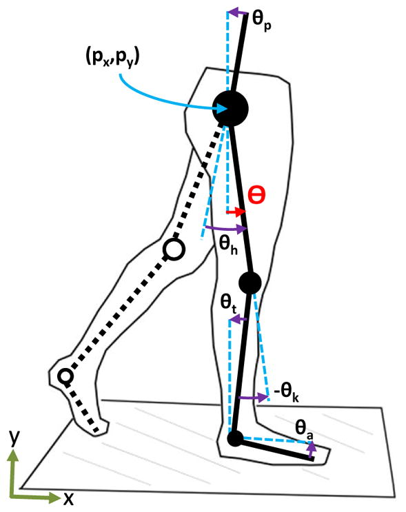
Body diagram of the leg coordinates p_x, p_y, θ_p, θ_h^, θ_k^{, and} θ_a corresponding to the horizontal hip position, vertical hip position, pelvic tilt, hip angle, knee angle, and ankle angle, respectively. The first three are global variables and the last three are relative variables. Additional global variables include the tibia angle θ_t and the thigh angle Θ, i.e., global hip angle. The horizontal hip position p_x and the polar coordinate of the thigh’s phase portrait are evaluated as phase variables.

We can obtain other global variables from these leg coordinates that may be useful as phase variables. The thigh angle, defined as the angle of the thigh with respect to the gravity vector, is obtained by Θ = θ_h − θ_p The tibia angle is similarly defined as θ_t = θ_k − Θ. The thigh angle, which we refer to as the global hip angle, will play an important role in computing the hip phase angle later in the paper.

B. Phase Variable Reparameterization

Given that biped dynamics are modeled as a second-order dynamical system via the Euler-Lagrange equations [12], the state of a leg at time t is given by the vector x(t):= (q(t), q̇(t)) ∈ ℝ¹². When the leg is in contact with the ground without slipping, there are 2 to 3 contact constraints that reduce the dimensionality of the system by constraining unactuated coordinates, e.g., horizontal/vertical translation [39]. The actuated coordinates, i.e., the leg joint angles and velocities, have rhythmic patterns during locomotion. We therefore define a projection ϖ: ℝ¹² → ℝ⁶ from the full state vector to the actuated subset z = ϖ(x) ∈ ℝ⁶. A steady walking gait with nominal trajectory x^*(t) = (q^*(t), q̇^*(t)) then has a periodic reference trajectory z^*(t) = ϖ(x^*(t)) = z^*(t + T ) for all t and some minimal period T > 0.

In gait analysis or control the projection of the current state x should match the current reference of the actuated coordinates, z^*. Typically, the current reference state is determined by the current time. That is, at time t, the reference point is z^*(t). This choice leads to two issues:

• I1In a single stride, if t > T then it is not clear what the reference should be. This could happen when taking longer steps than usual.
• I2Because time increases at a constant rate, the reference state z^* will always progress at this rate regardless of the actual state x. The reference gait cannot be slowed or accelerated in response to perturbations.

These issues can be overcome by using a phase variable instead of time to determine the current reference state. A phase variable φ is computed as a real-valued function f of the full state x. Thus, at time t, φ(t) = f(x(t)). In order for φ to be well-defined, it must satisfy two properties:

• P1Every state of the reference trajectory z^*(t) must correspond to a unique value of φ. This is guaranteed if φ(t) monotonically increases or decreases along a nominal trajectory x^*(t), i.e., the time-derivative of φ^*(t) = f(x^*(t)) is non-zero for all t.
• P2For any state x ∈ ℝ¹², the function f(x) ∈ I where I = {φ | φ= f(x^*(t)) for some t} is the set of phase values corresponding to a nominal trajectory x^*(t). This is guaranteed if the range of f(x) is equal to I.

These properties together allow us to use the current state x to determine the reference state z^*. We say that we have reparameterized the reference periodic trajectory z^*(t) by the phase variable φ = f(x). The current time is irrelevant to this procedure and φ is bounded in I, thus overcoming issue I1. If φ can be influenced by perturbations or volitional movement, then it is possible for the current value of φ to accurately represent the location in the gait cycle, which overcomes issue I2. In applications to prosthetic control, the human user could directly control the reference state of the prosthesis by moving a phase variable under his/her influence. In this paper we will derive such a variable related to the human hip joint.

C. Periodic Orbits and Stability

The periodic trajectory z^*(t) of a nominal walking gait defines a periodic orbit 𝒪:= {z|z = z^*(t) for some t} in the state space [40]. In the orbital sense of stability, the state z stays in a neighborhood of (or converges to) the orbit 𝒪 after perturbations. Phase is a time-invariant quantity equivalent to position along the periodic orbit. Mathematically, there exists a scalar function of the state that represents phase on the periodic orbit [41], but this function (the phase variable) is unknown for uncertain dynamics like that of human locomotion.

If the human gait cycle is orbitally stable, a perturbation along (or tangential to) the orbit will result in little to no response from the human, because the state will still be on or near the orbit. This is what we call a phase-shifting perturbation. A phase variable should shift up or down to characterize this change in position along the orbit. Evidence of orbital stability has been found by analyzing variability in non-perturbed human walking [42], but this work did not consider a representation of the location on the periodic orbit.

In this study we utilize translational perturbations to move the stance foot relative to the body’s center of mass as an approximation of a phase-shifting perturbation. Although this perturbation will cause slight deviations from the periodic orbit [32], the transient effects will be minimized by a proper phase parameterization. We consider these transient effects when forming our hypotheses in Section IV-B.

IV. Methods

In this section we derive a biologically meaningful monotonic phase variable that can be used for gait analysis and to control robotic prosthetic legs. We then state the hypotheses that will let us conclude whether certain phase variable parameterizations yield better results than a time-based parameterization when representing the behavior of joint trajectories during non-steady gait. Finally, we explain the experimental protocol used to investigate these hypotheses.

A. Deriving the Hip Phase Angle

We begin the phase variable derivation by examining a normative trajectory of the global hip angle Θ during human walking (see Section IV-C for data collection methods). The time derivative of the global hip angle, denoted as Θ̇, is computed numerically and filtered with a 5 Hz low-pass cutoff. A closed periodic orbit can be observed in the phase portrait of (Θ(t), Θ̇(t)) in Fig. 2 (left). The polar angle φ of the state on the periodic orbit can be computed as φ(t) = atan2(Θ̇(t), Θ(t)), where atan2 is the four-quadrant inverse tangent function. This function is bounded in [0, 2π) and therefore satisfies Property P2 to ensure the parameterization of the gait cycle is well-defined, i.e., all possible values of φ correspond to some reference state (Section III-B).

Fig. 2.

The natural and modified global hip kinematics used to compute the phase angle (i.e., polar coordinate of the phase portrait) are shown in the first two rows. The corresponding phase portrait and phase angle (φ) are shown in the last two rows.

The function φ is plotted in Fig. 2 (left) from the mean trajectory of Θ(t). The phase trajectory is very nonlinear and has a problematic non-monotonic region at the end, violating Property P1. Although linearity is not theoretically necessary for a phase variable, nonlinear regions of the phase trajectory can amplify the effect of sensor noise and should be minimized in practice. Hence, we redefine the phase variable as

$$\phi (t)=\text{atan}2(k\stackrel{.}{\mathrm{\Theta }}(t),\mathrm{\Theta }(t))$$ (1)

where k ∈ ℝ is chosen to make the phase portrait more circular so that φ(t) approximates a linear function of time (Fig. 2, right). Strict linearity can be achieved if Θ(t) is sinusoidal:

Theorem 1

If Θ(t) = a cos(ωt) for ω = 2πF, then φ(t) defined in (1) is strictly monotonic for any frequency ω and constant k. Moreover, if k = −1/ ω then φ(t) is also linear.

Proof

We first compute φ̇ and φ̈ to be

$$\stackrel{.}{\phi }(t)=-\frac{k{\omega }^2}{{cos}^2(\omega t)+k^2{\omega }^2{sin}^2(\omega t)}$$ (2)

$$\ddot{\phi }(t)=\frac{k{\omega }^3(k^2{\omega }^2-1)sin(2\omega t)}{{({cos}^2(\omega t)+k^2{\omega }^2{sin}^2(\omega t))}^2}.$$ (3)

It is clear from (2) that φ̇(t) ≠ 0 for any t regardless of constants k and ω, thus ensuring monotonicity. Letting k = −1/ω, then φ̇(t) = ω > 0 and φ̈(t) = 0 for all t, implying that φ(t) is linear and time-scaled by frequency ω.

This result would satisfy Property P1 to ensure that every state in the joint pattern corresponds to a unique value of the phase variable, even when the exact frequency is not known. The linearity result of Theorem 1, which is desirable for practical reasons, requires knowledge of frequency ω to compute k = −1/ω. The constant k can alternatively be computed from the range of motion of the phase portrait when Θ(t) = a cos(ωt):

$$\begin{array}{l}k=-\frac{\mid max(\mathrm{\Theta }(t))-min(\mathrm{\Theta }(t))\mid }{\mid max(\stackrel{.}{\mathrm{\Theta }}(t))-min(\stackrel{.}{\mathrm{\Theta }}(t))\mid }\\ =-\frac{\mid max(acos(\omega t))-min(acos(\omega t))\mid }{\mid max(-a\omega sin(\omega t))-min(-a\omega sin(\omega t))\mid }\\ =-\frac{\mid 2a\mid }{\mid 2a\omega \mid }=-\frac{1}{\omega }.\end{array}$$ (4)

Hence, the constant k can be computed every gait cycle to optimize linearity.

To leverage Theorem 1, the biomechanical variable Θ must have a nearly sinusoidal trajectory over the gait cycle. We chose the global hip angle because its correlation coefficient with respect to a cosine or sine signal is the largest (r = 0.943) of all the kinematic variables in Fig. 1. The relative hip angle θ_h is close behind (r = 0.936). Although the global tibia angle θ_t has been successfully used to control a prosthetic ankle in [28], it yields a smaller correlation coefficient (r = 0.778) than the global or relative hip angles. This analysis suggests that the phase portrait of the hip joint can be effectively transformed into a nearly monotonic and linear phase variable, as seen in Fig. 2 (bottom-right). The nonlinearity in the middle and the flat region at the end of the phase variable trajectory correspond to brief regions of the hip trajectory that deviate from a cosine signal. It is possible to improve the linearity of this region by computing the hip phase angle using the integral of Θ rather than the derivative [43], which will be discussed in Section VI. However, for our purposes the velocity-based hip phase angle is sufficiently monotonic to parameterize the vast majority of the human gait cycle. For convenience we normalize the phase variable between zero and one for the rest of the paper, i.e., φ = atan2(kΘ̇, Θ)/2π.

B. Hypotheses

1) Interjoint Coordination

We wish to determine whether the proposed phase variable can accurately parameterize leg joint trajectories during non-steady gait. The perturbation mechanism from [32] moves the stance leg relative to the body’s center of mass, which approximately shifts the stance leg joints to a previous or future configuration of their nominal kinematic orbits. If the gait cycle is orbitally stable, the leg joints would continue from this new location on their periodic orbits. In order to evaluate this behavior we compute the correlation coefficients between perturbed and non-perturbed joint angle trajectories amongst different parameterizations. In particular, we expect to see perturbed joint trajectories shifted backward or forward with respect to the nominal trajectories over time, depending on the perturbation direction. However, when the joint angles are reparameterized by a robust phase variable, the shift would be captured by the phase variable resulting in perfectly overlapping trajectories. Therefore, correlation coefficients are expected to be consistently greater over a proper phase variable than over time, otherwise the phase variable does not provide a robust parameterization of the human gait cycle.

Hypothesis 1 (H1)

The correlation coefficients between perturbed and nominal joint trajectories will be greater (and less variable) when parameterized by hip phase angle than by time or hip position. In addition, the coefficients from the hip phase angle parameterization will be marginally close to one.

Because we cannot perturb the leg state perfectly tangential to the periodic orbit (i.e., a pure phase-shift), we should expect some transient effects in the experimental data [32]. If the periodic orbit is stable, the leg state would remain in a neighborhood around (or converge to) the periodic orbit after a perturbation that does not stop the cycle. A phase variable that properly represents the location on the orbit would consistently minimize the transient error observed between the perturbed and nominal joint trajectories when parameterized by that variable. The total observed error can be quantified by the Root Mean Squared (RMS) value of the observed error trajectory.

Hypothesis 2 (H2)

The RMS errors between perturbed and nominal joint trajectories will be smaller (and less variable) when parameterized by hip phase angle than by time or hip position.

2) Interlimb Coordination

A topic of inquiry in human locomotor control is the manner of coordination between legs, e.g., how sensory feedback from one leg affects the control of the other. In this study we wish to determine how the phasing of one leg affects the phasing of the other. We define an ipsilateral parameterization of one leg’s joints using a phase variable from the same leg, whereas a contralateral parameterization of one leg’s joints may utilize the other leg’s phase variable (e.g., swing leg joints parameterized by the stance leg phase variable). Identifying the most robust parameterization (ipsilateral vs. contralateral) may give clues about the underlying feedback control architecture behind human locomotion. The robustness of each parameterization can be tested by shifting the phase of one leg relative to the other leg using the same perturbations described for H1–H2. These phase shifts will also show how the legs ultimately synchronize to maintain coordination. The correlation coefficients and RMS errors can be used to compare and draw conclusions about these two interlimb phase parameterizations.

Hypothesis 3 (H3)

The ipsilateral hip phase angle will provide the greatest correlation coefficients and smallest RMS errors between the perturbed and nominal joint trajectories of each leg.

C. Experimental Protocol

The perturbation platform from [32] was embedded in the middle of an 8 m walkway (Fig. 3). A force plate (Kistler, Winterthur, Switzerland) was placed on top of the platform to detect foot contact. The top of the force plate was level with the walkway surface. The perturbation platform was designed to move the stance foot 5 cm forward or backward in 100 ms [32]. This perturbation magnitude and duration were specifically chosen to cause an abrupt phase shift along the periodic orbit. The gait cycle was accelerated or decelerated by moving the stance foot behind or ahead of the body, respectively. A total of ten motion capture cameras (Vicon, Oxford, UK) were used to capture the kinematics of the subject walking. After experiments the joint kinematics were processed using Vicon Nexus Plug-in-Gait software.

Fig. 3.

Top view of the experimental setup. The subject walked along an 8 m walkway, stepping on the force plate in the center. The force plate randomly translated forward or backward 5 cm over 100 ms at different times after heel contact, moving the stance leg ahead or behind the body, respectively. The subject was asked to walk naturally from the starting position to the final position, after which the subject turned around and repeated.

The experimental protocol was reviewed and approved by the Institutional Review Board (IRB) at The University of Texas at Dallas. A total of ten able-bodied subjects (6 male and 4 female) were enrolled in the study. The experiment involved four sets of 72 trials (288 trials in total) for each subject. Each trial consisted of the subject walking from a fixed starting point, stepping with their right foot on the force plate in the middle of the walkway, and continuing to walk until the end of the walkway (Fig. 3). Although force plate targeting does not significantly alter gait kinetics or kinematics [44]–[46], the subject was given time before data collection to find a preferred starting point on the walkway to achieve consistent, clean contact on the force plate with minimal targeting. Handrails were located along the walkway to mitigate the risk of falling, but no subject used them at any time during the experiment.

When a subject stepped on the perturbation mechanism, one of seven possible conditions would randomly occur: 1) forward perturbation after a 100 ms delay (100fwd), 2) backward perturbation after 100 ms delay (100bwd), 3) forward perturbation after 250 ms delay (250fwd), 4) backward perturbation after 250 ms delay (250bwd), 5) forward perturbation after 500 ms delay (500fwd), 6) backward perturbation after 500 ms delay, and 7) no perturbation (NP). At these specific times, the hip, knee, and ankle joints are typically in a monotonic region of the angular trajectories as will be seen later [1]. Thus a perturbation at these instants would not cause the joints to deviate much from their nominal periodic orbits [32]. To prevent anticipatory compensations from the subjects, the perturbation conditions 1–6 were randomized with a probability of 0.083 each, whereas no perturbation (condition 7) occurred with a probability of 0.5. A supplemental video of these perturbation conditions is available for download.

D. Statistical Analysis

The correlation coefficients between average perturbed and average non-perturbed joint angle trajectories were computed using MATLAB (MathWorks, Massachusetts, USA) for each perturbation condition per subject. The correlation coefficient averaged across all types of perturbations was calculated in order to have a single metric per subject capable of quantifying the performance of each parameterization. We consider that despite the type of perturbation the correlation coefficient can measure how well any of the leg joint angles followed their nominal (non-perturbed) joint trajectory (see Section IV-B). An upper-tail t-test was used to statistically compare the correlation coefficients of the time-based and two phase variable parameterizations of the joint angle trajectories between perturbed and non-perturbed conditions. A p-value less than 0.05 in this test would correspond to a statistically greater correlation coefficient for one parameterization than another parameterization, by which we tested H1 and H3.

A lower-tail t-test was used to compare the observed transient error between parameterizations. The observed transient error was quantified by the RMS error between the average perturbed joint trajectories and the average non-perturbed joint trajectories for each parameterization per subject. An overall error was calculated by averaging the RMS errors across all types of perturbations. This averaged RMS error provides a single metric capable of describing the transients of one subject across all the perturbations. A p-value less than 0.05 in this analysis would correspond to a statistically smaller transient response observed for one parameterization than another, by which we tested H2 and H3.

A correlation coefficient equal to one between perturbed and non-perturbed joint trajectories would imply a perfect overlap of the joint trajectories, which is desired in a proper phase parameterization. However, it is not possible to achieve a perfect correlation coefficient from experimental data due to noise, misaligned markers, or general variability. Therefore, a 95% lower confidence interval (CI) on the correlation coefficient between perturbed and non-perturbed joint angle trajectories was calculated for each parameterization to further test H1. This CI informs on how statistically close the correlation coefficient can approach the value of one for each parameterization. Similarly for H2, an upper bound CI was computed for the RMS error to measure the closeness of the error to a value of zero.

Finally, a lower-tail F-test is used to determine whether the correlation coefficients and RMS errors have a smaller standard deviation (SD) in the phase angle parameterization as proposed in H1 and H2. This would suggest that the trajectories are consistently represented in the parameterization.

V. Results

A. Interjoint Coordination

Visual inspection of Figs. 4 and 5 reveals that the hip phase angle parameterized the perturbed joint trajectories substantially better than both time and hip position. The parameterizations by time and hip position show a clear phase shift of the joint trajectories caused by each perturbation. No phase shift is observed in the hip phase angle parameterization, indicating that the phase shift was accurately captured by the hip phase angle. This phase shift in the hip phase angle is clearly seen in Fig. 6. The phase angle deviated from its nominal trajectory during the perturbation duration (100 ms) and then continued parallel to the nominal trajectory until reaching the same end-point value (one), earlier or later in time depending on the perturbation direction.

Fig. 4.

The hip, knee, and ankle joint angles (top, middle, and bottom rows) for the initiating leg (i.e., leg contacting the perturbation platform) are shown parameterized over time (left), hip position (center), and hip phase angle (right) for 100 ms onset condition. The blue solid line represents the non-perturbed trajectories, whereas the red dashed and green dash-dot lines represent the joint trajectories perturbed backward (i.e., moving stance leg behind the body) and forward (i.e., moving stance leg ahead of the body). The black dashed vertical line represents the onset time of the perturbation.

Fig. 5.

The hip, knee, and ankle joint angles (top, middle, and bottom rows) for the initiating leg (i.e., leg contacting the perturbation platform) are shown parameterized over time (left), hip position (center), and hip phase angle (right) for 250 ms onset condition. The blue solid line represents the non-perturbed trajectories, whereas the red dashed and green dash-dot lines represent the joint trajectories perturbed backward (i.e., moving stance leg behind the body) and forward (i.e., moving stance leg ahead of the body). The black dashed vertical line represents the onset time of the perturbation.

Fig. 6.

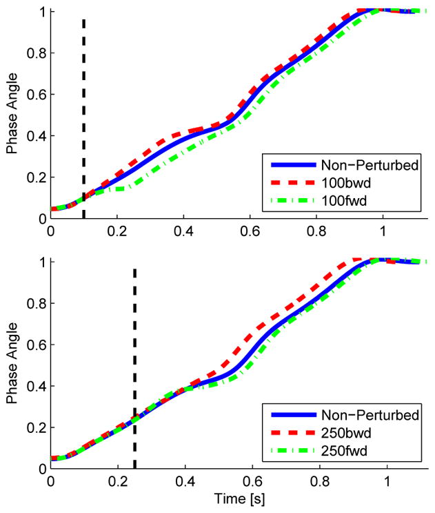
Hip phase angle over time with and without perturbations at 100 ms (top) and 250 ms (bottom) after initial contact with the platform. The dashed red line shows the backward perturbation condition (i.e., moving stance leg behind the body), whereas the dash-dot green line shows the forward perturbation condition (i.e., moving stance leg ahead of the body). The dashed black vertical line represents the onset time of the perturbation.

The perturbation responses appear similar for both the 100 ms and 250 ms onset conditions. The perturbation occurring at 500 ms after initial contact did not produce any noticeable kinematic changes. This could be due to the perturbation occurring during the double support period, which may make the subject’s gait robust against perturbations to the trailing stance leg. Thus, the 500 ms onset condition was excluded from the statistical analysis.

Across subjects the parameterization by hip phase angle yielded the highest correlation coefficients per joint. The sample means and SDs for each parameterization are given in Table I. When conducting upper-tail t-tests on the inter-subject correlation coefficients between parameterizations, the p-values for the phase angle parameterization were found to be smaller than the confidence value of 0.05 (Table II). These p-values support the claim in H1 that the correlation coefficients are greater when the joint trajectories are parameterized by the hip phase angle than by time or hip position. Moreover, the t-tests found no statistical difference between the parameterizations of hip position and time, suggesting that hip position is not a robust representation of phase for human locomotion.

TABLE I.

Correlation and RMS Error Across Parameterizations

	Time Parameterization
	Hip		Knee		Ankle
	Corr	Error	Corr	Error	Corr	Error
Mean	0.959	4.094	0.959	5.356	0.862	4.333
SD	0.048	1.265	0.052	1.433	0.119	1.028
CI	0.931	4.826	0.929	6.185	0.793	4.928
	Hip Position Parameterization
Mean	0.974	4.101	0.976	5.143	0.905	3.986
SD	0.014	1.447	0.011	1.514	0.040	0.964
CI	0.966	4.939	0.970	6.020	0.882	4.544
	Hip Phase Angle Parameterization
Mean	0.997	1.459	0.995	2.476	0.955	2.795
SD	0.002	0.200	0.002	0.602	0.027	0.451
CI	0.996	1.575	0.994	2.824	0.940	3.056

The mean values, SD, and lower CI of the correlation coefficients and RMS errors between the perturbed and non-perturbed trajectories for each joint across parameterizations.

TABLE II.

Statistical Analysis on the Correlation Coefficient

Across Subject Statistical Analysis (p-values)
Mean (t-test)	Hip	Knee	Ankle
Hip Pos. > Time	0.177	0.169	0.146
Phase Angle > Time	0.016*	0.028*	0.018*
Phase Angle > Hip Pos.	≪0.05	≪0.05	0.003*
SD (F-test)	Hip	Knee	Ankle
Hip Pos. < Time	0.001*	≪0.05	0.002*
Phase Angle < Time	≪0.05	≪0.05	≪0.05
Phase Angle < Hip Pos.	≪0.05	≪0.05	0.130

P-values per joint from upper-tail t-tests on the mean (top) and lower-tail F-tests on the SD (bottom) of cross-subject correlation coefficients between parameterizations.

P-values that are less than the confidence level 0.05 are represented by (*) and p-values that are considerably smaller than this level are represented by ≪0.05.

The hip phase angle also maximized the correlation coefficient’s closeness to one and minimized its variability compared to the other parameterizations. A lower-bound 95% CI of the correlation coefficient was computed for each parameterization, showing the minimum statistical value of the correlation coefficient (Table I). The lower-bound CI of the hip phase angle’s coefficient reaches a value as high as 0.99, whereas the time and hip position parameterizations reach values of 0.94 and 0.96, respectively. Hence, the correlation coefficient of the phase angle parameterization is approximately equal to one as predicted in H1. Moreover, the SD of the correlation coefficients is smaller in the phase-based parameterizations than in the temporal parameterization. The lower-tail F-tests between the phase-based and time-based correlation coefficients in Table II indicate that the perturbed trajectories are more consistently correlated with the nominal trajectories when reparameterized by a phase variable. The hip phase angle yielded the smallest SD amongst all parameterizations.

The error observed between the perturbed and non-perturbed joint trajectories was smaller and less variable over the hip phase angle than over time, Fig. 7. The RMS values of these error trajectories quantify how well the parameterization captures the convergence of the joint angles back to their periodic orbit after a perturbation. Table I shows the mean and SD of these RMS errors for all parameterizations. The lower-tail t-tests in Table III indicate that the RMS errors are statistically smaller when the joint trajectories are parameterized by the phase angle than by time or hip position, which supports H2. In addition, the SD of the RMS error was statistically smaller in the phase angle parameterization according to the lower-tail F-test in Table III. These analyses suggest that the hip phase angle accurately and consistently represents the location of the human subject in his/her stable periodic orbit, whereas time and hip position do not. A supplemental data file contains the joint-specific correlation coefficients and RMS errors per parameterization for each human subject.

Fig. 7.

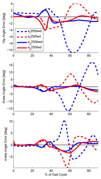
Observed errors between perturbed and nominal joint trajectories in the time parameterization (e_t) vs. the hip phase angle parameterization (e_p) for the initiating leg with the 250 ms onset condition. The observed errors of the phase parameterization tend toward zero. The last 10% of the gait cycle was excluded because ground impact prevents strict monotonicity, preventing the interpolation of joint trajectories to compute the phase-based error.

TABLE III.

Statistical Analysis on the RMS Error

Across Subject Statistical Analysis (p-values)
Mean (t-test)	Hip	Knee	Ankle
Hip Pos. < Time	0.495	0.375	0.224
Phase Angle < Time	≪0.05	≪0.05	≪0.05
Phase Angle < Hip Pos.	≪0.05	≪0.05	0.002*
SD (F-test)	Hip	Knee	Ankle
Hip Pos. < Time	0.650	0.560	0.430
Phase Angle < Time	≪0.05	0.008*	0.010*
Phase Angle < Hip Pos.	≪0.05	0.006*	0.020*

P-values per joint from lower-tail t-tests on the mean (top) and lower-tail F-tests on the SD (bottom) of cross-subject RMS errors between parameterizations.

B. Interlimb Coordination

The correlation coefficients and RMS errors were computed for ipsilateral and contralateral phase angle parameterizations. In particular, each leg’s hip phase angle was used to parameterize the respective leg’s joint angles (ipsilateral hypothesis) or the opposite leg’s joint angles (contralateral hypothesis). For this analysis we consider only the step when the initiating (stance) leg is in contact with the force plate, rather than a complete gait cycle. Fig. 8 shows the non-initiating (swing) leg during the perturbation step parameterized by ipsilateral and contralateral phase angles. Tables IV and V show the across-subject mean values associated with the correlation coefficients and RMS errors for each interlimb parameterization. The ipsilateral phase angle parameterizes the joint angles more consistently across perturbations.

Fig. 8.

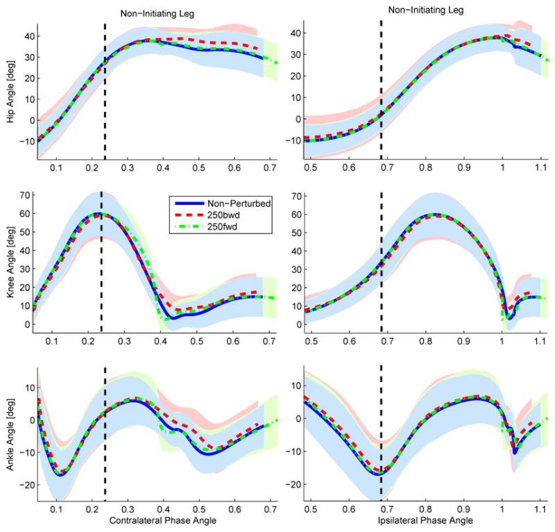
Contralateral (left) vs. ipsilateral (right) hip phase angle parameterizations of the non-initiating (i.e., swing) leg during the perturbation step for the 250 ms onset condition. The blue solid line represents the non-perturbed trajectories, whereas the red dashed and green dash-dot lines represent the backward and forward perturbation conditions, respectively. The black dashed vertical line represents the onset time of the perturbation. Note that the ranges of the contralateral and ipsilateral phase variables differ by 0.5 because of the anti-phasic relationship between the stance and swing legs.

TABLE IV.

Correlation Coefficients for Interlimb Coordination

	PV(Swing) - Swing Joints			PV(Swing) - Stance Joints
	Hip	Knee	Ankle	Hip	Knee	Ankle
Mean	0.996	0.970	0.915	0.987	0.741	0.839
SD	0.005	0.031	0.086	0.010	0.203	0.119
	PV(Stance) - Swing Joints			PV(Stance) - Stance Joints
	Hip	Knee	Ankle	Hip	Knee	Ankle
Mean	0.983	0.910	0.856	0.995	0.894	0.939
SD	0.013	0.075	0.152	0.002	0.164	0.052

The correlation coefficients per joint are shown for different interlimb parameterizations. PV(XX) - YY represents the joints of leg YY parameterized by the phase angle of leg XX.

TABLE V.

RMS errors for Interlimb Coordination

	PV(Swing) - Swing Joints			PV(Swing) - Stance Joints
	Hip	Knee	Ankle	Hip	Knee	Ankle
Mean	2.178	4.863	4.637	2.820	4.093	3.654
SD	1.062	2.290	4.089	1.310	1.600	1.849
	PV(Stance) - Swing Joints			PV(Stance) - Stance Joints
	Hip	Knee	Ankle	Hip	Knee	Ankle
Mean	3.333	7.681	4.848	1.960	2.002	2.319
SD	1.088	1.975	4.016	0.349	0.438	0.498

The RMS errors per joint are shown for different interlimb interlimb parameterizations. PV(XX) - YY represents the joints of leg YY parameterized by the phase angle of leg XX.

Fig. 9 shows the swing-to-stance transition of the non-initiating leg with and without perturbations that occurred 250 ms after contact of the initiating leg. The joint kinematics of the non-initiating leg are unaffected by the perturbation while in swing. From Figs. 8 and 9 it can be seen that, after a perturbation, the non-initiating leg synchronizes with the phase of the initiating leg during the double-support period. This result would suggest that the stance leg rules, in some sense, over the synchronization of locomotion and that double-support is needed to synchronize both leg’s phase variables.

Fig. 9.

The swing-to-stance transition of the non-initiating leg (i.e., contralateral to the stance leg in contact with the force plate) shown parameterized over time for the 250 ms onset condition. The blue solid line represents the non-perturbed trajectories, whereas the red dashed and green dash-dot lines represent the backward and forward perturbation conditions, respectively. The black dashed vertical line represents the onset time of the perturbation whereas the blue solid, red dashed, and dash-dot green vertical lines represent the stance-to-swing transition of the contralateral (initiating) leg.

Tables VI and VII show the results of the upper-tail t-tests of the claim in H3 that the ipsilateral phase angle provides the greatest correlation coefficients and smallest RMS errors. The majority of the p-values are less than the confidence level of 0.05, thus supporting H3 (i.e., a phase variable local to each leg). The supplemental data file contains the subject-specific values used for this statistical analysis.

TABLE VI.

Statistical Analysis on Interlimb Correlation

Ipsilateral > Contralateral Parameterization
Leg	Hip	Knee	Ankle
Swing	0.007*	0.019*	0.151
Stance	0.016*	0.040*	0.015*

The p-values per joint from upper-tail t-tests on the cross-subject correlation coefficients being larger for an ipsilateral parameterization.

TABLE VII.

Statistical Analysis on Interlimb RMS Error

Ipsilateral < Contralateral Parameterization
Leg	Hip	Knee	Ankle
Swing	0.014*	0.004*	0.454
Stance	0.036*	0.001*	0.026*

The p-values per joint from lower-tail t-tests on the cross-subject RMS errors being smaller for an ipsilateral parameterization.

VI. Discussion

For the most part, the hip phase angle fulfilled the requirements of a phase variable established in Sections III-B and IV-A. We computed this phase variable from the global hip angle because of its close resemblance to a cosine function during the gait cycle, but the relative hip angle may also be a suitable choice. The trajectory of the hip phase angle appears bounded, monotonic, and mostly linear in Fig. 6. There is, however, a short region at the beginning and end of the gait cycle where this variable loses strict monotonicity because of the high velocities associated with the impact of heel strike, which briefly violate the assumption of a sinusoidal signal in Theorem 1. This only presented a limitation when computing the last 10% of the phase-based error in Fig. 7. The last 10% of the gait cycle can be better captured by computing the phase angle with the integral of the hip angular position rather than the derivative [43], which will be discussed later.

Our experiments verify that the hip phase angle is able to represent changes in gait cycle phase across perturbations at different points in the gait cycle. It can be seen in Fig. 6 that a backward perturbation (moving the stance leg behind the subject’s center of mass) accelerated the progression of the phase angle and thus the phase angle arrived at its endpoint value (one) in less time than without the perturbation. The opposite behavior occurred in response to a forward perturbation. In other words, the behavior of the phase angle correlates well with the step period across perturbations.

A. Interjoint Coordination

By accurately reflecting phase shifts, the hip phase angle helps visualize the synchronization of the joint kinematics across perturbations (Figs. 4 and 5). In contrast, the perturbed joint trajectories do not overlap with the nominal trajectories when parameterized by time or hip position because those variables do not accurately characterize phase shifts.

The correlation coefficients for H1 quantify how well the phase variable represents the location of the leg state on the periodic orbit. These coefficients were higher than 0.95 for the hip phase angle parameterization, confirming that the phase shift along the periodic orbit was accurately captured. The joint trajectories in Figs. 4 and 5 show that the perturbation was not exactly tangential to the periodic orbit, causing a small transient response that is better viewed in Fig. 7.

The RMS errors for H2 characterize the ability of a phase variable to represent transient behavior (such as convergence) off the periodic orbit. The observed errors between perturbed and non-perturbed joint trajectories were smallest when parameterized by hip phase angle. The observed error of this parameterization tends to zero in Fig. 7, whereas the time-based error clearly does not converge. This provides evidence of orbital stability, where the hip phase angle represents the location on the orbit. The ability of this variable to parameterize transient responses also suggests that it may be robust to other types of perturbations encountered during walking.

B. Interlimb Coordination

Interlimb phasing does not appear to synchronize until the double support period. The perturbation to the initiating (stance) leg is not visible in the non-initiating leg during swing (Fig. 9). This phase difference between legs disappears during the double-support period, after which the non-initiating leg (now in stance) has synchronized to the phase of the initiating leg (now in swing). This suggests that the stance leg might be in control of the overall phase of the gait cycle, i.e., the swing leg (leading leg) adopts the phase of the stance leg (trailing leg) at the end of a step.

The statistical tests for H3 (Table VI) support an ipsilateral parameterization of the legs, i.e., each leg parameterized by its own hip phase angle. A proper parameterization of the joint trajectories of the non-initiating leg (i.e., swing leg) should respect the fact that this leg was not affected during the perturbation step as seen in Fig. 9. However, the contralateral parameterization (based on the stance hip phase angle) in Fig. 8 seems to artificially perturb the swing leg. This behavior is not present in the ipsilateral parameterization, suggesting that the progression of the swing joint angles is represented better by the ipsilateral phase angle.

The swing ankle joint has the only p-value greater than the confidence level in Table VI. This could be due to the ankle’s variability. A previous study found that the variability of the ankle does not correlate to the variability of the other leg joints [47]. It seems that the swing ankle could be acting passively or under the influence of local reflexes that are not well characterized by the phase angle of either hip joint.

C. Biological Implications

These results suggest that the human neuromuscular system may independently encode the phase of each leg via ipsilateral sensory feedback, which could be related to each leg’s hip phase angle. These two senses of phase become synchronized when physically constrained by the ground during double support. Thus human legs may be coordinated primarily by ground contact. This biological hypothesis of interlimb coordination contrasts with the standard method of controlling biped robots with a master phase variable related to the stance leg [12].

The interjoint coordination results align with the concept of “proximal controls distal” in [48], where Popović et al. found that shoulder flexion/extension strongly predicts elbow flexion/extension and forearm pronation/supination during hand manipulation tasks. The shoulder joint angle was then proposed as a control input to a neural prosthesis for stimulating elbow and forearm motion [48]. Analogously, we have found that hip phasing strongly predicts knee and ankle phasing. In particular, the correlations in the hip phase angle parameterization were very similar for the hip and knee joints (0.99+), whereas the correlation decreased only slightly to 0.955 at the ankle (Table I). Hip motion could thus be used as an input for controlling distal leg joints in prosthetics applications, which will be discussed in Section VI-D.

Our results can also be interpreted in terms of a “proximo-distal gradient” control architecture governing the gait cycle [10], [49]. The proximo-distal gradient hypothesis states that the more proximal joints are more influenced by feedforward signals from the spinal cord, whereas the more distal joints are more influenced by local force feedback loops. Along these lines, it is possible that feedforward signals kept the phasing of the hip and knee joints highly correlated across perturbations. However, these feedforward signals must have been quickly modulated by afferent feedback from the hip to produce the phase shifts observed after perturbations. The presence of positive force feedback loops about the ankle joint [50] could explain why this joint had the smallest correlation coefficient and greatest RMS error in the hip phase angle parameterization (Table I). It is possible that a COP-based parameterization of the stance ankle pattern [22] could better account for these force feedback loops, but the limitation of the COP to the stance period prevented us from directly comparing it with the hip phase angle across the gait cycle.

Regardless of the underlying neuromechanics, the hip phase angle appears to provide a very robust parameterization of the human gait cycle and thus could be particularly useful in gait studies. Perturbation studies of rhythmic behavior are limited by the lack of an observable variable that uniquely represents the cycle phase after a perturbation or stimulus [9]. Although phase is equivalent to time during steady gait, a perturbation can alter the progression of phase, e.g., slowing or accelerating the gait pattern. Time still advances at a constant rate, so the conventional gait cycle percentage (time normalized between discrete events) distorts the deviation between perturbed and nominal kinematics (left sides of Figs. 4 and 5). An observable representation of phase like the hip phase angle is needed to view the transient response from the perspective of the human body. This approach is related in principle to the method of dynamic time warping [51], which scales time to better match kinematic profiles (e.g., for gait recognition [52]). However, the “similarity searches” involved in dynamic time warping are non-causal so do not provide a real-time measure of the body’s progression like a phase variable does.

D. Robotics Implications

These results also have implications on the selection of phase variables for legged robots. The majority of dynamic walking robots control their joint patterns using the stance leg angle (i.e., hip position) as a phase variable [12]. This worked well for sagittal-plane biped models, but only recently was it realized that the choice of phase variable has substantial implications on the stability of 3D walking [19]. The choice of stance leg angle results in a difficult stabilization problem that requires event-based control updates to achieve stable 3D walking [18]. Biped robots could possibly be made more robust and human-like by instead controlling joint patterns with the hip phase angle. This also begs the question as to whether biped robots could benefit from ipsilateral interleg phasing as opposed to the current paradigm of a master phase variable associated with the stance leg.

Wearable robots like powered prostheses and orthoses could also benefit from a human-like sense of phase. Powered prostheses and orthoses almost universally use several control modes in a finite state machine (FSM) representation of the gait cycle [5], where switching rules or estimates of gait cycle phase (typically relying on several sensors) determine when to switch between control modes. Determining the correct timing of events based on the human’s motion is crucial to the operation of these devices. The hip phase angle could provide an accurate and easy-to-measure estimate of the human’s gait cycle phase for these control strategies. More recent unified control strategies for prosthetic legs [21], [24], [27] could also use the hip phase angle to parameterize joint trajectories for the entire gait cycle (see initial work in [53]). By controlling joint patterns as continuous functions of the hip phase angle, prosthetic legs could better match the phase of the human user and consequently respond to perturbations in predictable human-like manner.

Although the hip phase angle can be easily computed offline from post-processed kinematic data, its dependence on angular velocity presents a challenge for real-time computation in a prosthetic control system. Angular velocity is very susceptible to noise from impacts, which we saw affects the linearity of the phase variable (Fig. 6). Filtering this noise would introduce undesirable phase lag in the real-time controller. Furthermore, a phase variable that depends on velocity is only one derivative away from the equations of motion, i.e., relative degree-one [54], which prevents the use of derivative error corrections in the controller. Recent work [43] introduces relative degree-two alternatives to the velocity-based hip phase angle, including a phase angle computed from the hip angle and its integral. The integral-based hip phase angle is more robust to noise and more linear (even the last 10% of the gait cycle), which facilitated implementation in a powered knee-ankle prosthesis in [53]. However, the analysis in [43] found that human joint kinematics are parameterized more accurately by the velocity-based phase angle considered in the present paper.

E. Study Limitations

The experimental protocol of targeting the perturbation platform during overground walking could be considered a limitation of the study. We do not believe that knowledge of the perturbation mechanism significantly affected the results. Previous studies have shown that the kinetics, ground reaction forces, and kinematics are not altered by targeting a force plate [44]–[46]. Our experimental protocol also randomized all perturbation conditions with an increased probability of no perturbation to prevent anticipatory compensations. Hence, even if the human subjects were conscious of the perturbation mechanism, it was impossible to correct their kinematics in favor of a specific type of perturbation. Analysis of EMG recordings also did not find abnormal co-contraction other than during the swing-to-stance transition [32], which occurred before the perturbations and thus did not affect the perturbation responses. Although known treadmills cannot accelerate as quickly as our perturbation mechanism, future experiments with pseudo-random perturbations on an instrumented split-belt treadmill may verify these overground findings.

VII. Conclusion

In this paper a robust phase variable (the hip phase angle) was derived analytically and validated by perturbation experiments with human subjects. A statistical analysis comparing the perturbed and non-perturbed joint kinematics concluded that the hip phase angle is a better parameterization of the gait cycle than time and a different phase variable. An analysis of interlimb coordination supported an ipsilateral phase parameterization, where each leg has a local hip phase angle. The derivation and validation of this phase variable provides 1) a biologically meaningful representation of phase to analyze non-steady gait, 2) a real-time measure of phase for controlling wearable robots in synchrony with human limbs, and 3) possible insight into the underlying control mechanisms behind human locomotion. The fact that the hip phase angle was derived from a single measurement will facilitate its implementation in wearable robots. Future work will involve verifying these results with quasi-random treadmill perturbations and using the hip phase angle to control a robotic prosthetic leg (see [53]).

Biographies

Dario J. Villarreal (S’13) received the B.Eng. degree (2012) in mechatronics engineering from the Saltillo Institute of Technology and is currently pursuing a Ph.D. in Biomedical Engineering at the University of Texas at Dallas. He is a recipient of the CONACYT Fellow. His current research interests include biomechatronics, robotics, systems and controls, neuromechanics, and gait analysis with emphasis on powered transfemoral prosthesis.

Hasan A. Poonawala (S’14-M’15) received the B.Tech. degree in mechanical engineering from the National Institute of Technology, Surathkal, India, in 2007, the M.S. degree in mechanical engineering from the University of Michigan, Ann Arbor, MI, USA, in 2009, and the Ph.D. degree in electrical engineering from the University of Texas, Dallas, TX, USA, in 2014. He is currently a postdoctoral researcher at the University of Texas at Austin. His current research interests include robotics, networked systems and nonlinear control theory.

Robert D. Gregg (S’08-M’10-SM’16) received the B.S. degree (2006) in electrical engineering and computer sciences from the University of California, Berkeley and the M.S. (2007) and Ph.D. (2010) degrees in electrical and computer engineering from the University of Illinois at Urbana-Champaign.

He joined the Departments of Bioengineering and Mechanical Engineering at the University of Texas at Dallas (UTD) as an Assistant Professor in 2013. Prior to joining UTD, he was a Research Scientist at the Rehabilitation Institute of Chicago and a Postdoctoral Fellow at Northwestern University. His research is in the control of bipedal locomotion with applications to autonomous and wearable robots.

References

- 1.Winter D. Biomechancis and Motor Control of Human Movement. J. Wiley and S. Inc, Eds; Hoboken, NJ: 2009. [Google Scholar]
- 2.Perry J, Burnfield J. Gait Analysis Normal and Pathological Function. Slack-Incorporated, Ed; Thorofare, NJ: 2010. [Google Scholar]
- 3.Sup F, Bohara A, Goldfarb M. Design and control of a powered transfemoral prosthesis. Int J Robotics Research. 2008 Feb;27(2):263–273. doi: 10.1177/0278364907084588. [DOI] [PMC free article] [PubMed] [Google Scholar]
- 4.Kazerooni H, Steger R, Huang L. Hybrid control of the berkeley lower extremity exoskeleton (BLEEX) Int J Robotics Research. 2006 May;25(5–6):561–573. [Google Scholar]
- 5.Tucker MR, Olivier J, Pagel A, Bleuler H, Bouri M, Lambercy O, del J, Millán R, Riener R, Vallery H, Gassert R. Control strategies for active lower extremity prosthetics and orthotics: a review. J Neuroengineering and Rehabilitation. 2015;12(1):1–29. doi: 10.1186/1743-0003-12-1. [DOI] [PMC free article] [PubMed] [Google Scholar]
- 6.Tilton AK, THsiao-Wecksler E, Mehta PG. Filtering with rhythms: Application to estimation of gait cycle,” in. American Control Conference. 2012:3433–3438. [Google Scholar]
- 7.Taghvaei A, Hutchinson SA, Mehta PG. A coupled oscillators-based control architecture for locomotory gaits. IEEE Conf. Decision & Control; 2014; pp. 3487–3492. [Google Scholar]
- 8.Revzen S, Guckenheimer J. Estimating the phase of synchronized oscillators. Physical Review E. 2008;78(5):051907. doi: 10.1103/PhysRevE.78.051907. [DOI] [PubMed] [Google Scholar]
- 9.Vogelstein RJ, Etienne-Cummings R, Thakor NV, Cohen AH. Phase-dependent effects of spinal cord stimulation on locomotor activity. IEEE Trans Neural Sys Rehab Eng. 2006 Sep;14(3):257–65. doi: 10.1109/TNSRE.2006.881586. [DOI] [PubMed] [Google Scholar]
- 10.Dzeladini F, Van Den Kieboom J, Ijspeert A. The contribution of a central pattern generator in a reflex-based neuromuscular model. Frontiers in Human Neuroscience. 2014;8(371) doi: 10.3389/fnhum.2014.00371. [DOI] [PMC free article] [PubMed] [Google Scholar]
- 11.Ronsse R, Vitiello N, Lenzi T, van den Kieboom J, Carrozza MC, Ijspeert AJ. Human–robot synchrony: flexible assistance using adaptive oscillators. IEEE Trans Biomed Eng. 2011;58(4):1001–1012. doi: 10.1109/TBME.2010.2089629. [DOI] [PubMed] [Google Scholar]
- 12.Grizzle J, Westervelt E, Chevallereau C, Choi J, Morris B. Feedback Control of Dynamic Bipedal Robot Locomotion. Boca Raton, FL: CRC Press; 2007. [Google Scholar]
- 13.Grizzle JW, Abba G, Plestan F. Asymptotically stable walking for biped robots: analysis via systems with impulse effects. IEEE Transactions on Automatic Control. 2001;46(3):513–513. [Google Scholar]
- 14.Sreenath K, Park H-W, Poulakakis I, Grizzle J. A compliant Hybrid Zero Dynamics controller for stable, efficient and fast bipedal walking on MABEL. Int J Robotics Research. 2010 Sep;30(9):1170–1193. [Google Scholar]
- 15.Powell MJ, Zhao H, Ames AD. Motion primitives for human-inspired bipedal robotic locomotion: walking and stair climbing. IEEE Int. Conf. Robotics and Automation; May 2012.pp. 543–549. [Google Scholar]
- 16.Ramezani A, Hurst J, Hamed K, Grizzle J. Performance analysis and feedback control of ATRIAS, a three-dimensional bipedal robot. ASME J Dyn Sys Meas Control. 2013;136(2):021012. [Google Scholar]
- 17.Buss B, Ramezani A, Hamed K, Griffin B, Galloway K, Grizzle J. Preliminary walking experiments with underactuated 3d bipedal robot marlo. IEEE Int. Conf. Intelli. Robots Sys; 2014. [Google Scholar]
- 18.Hamed KA, Grizzle JW. Event-based stabilization of periodic orbits for underactuated 3-d bipedal robots with left-right symmetry. IEEE Trans Robotics. 2014;30(2):365–381. [Google Scholar]
- 19.Hamed KA, Buss BG, Grizzle JW. Continuous-time controllers for stabilizing periodic orbits of hybrid systems: Application to an underactuated 3D bipedal robot. IEEE Conf. Decision & Control; 2014; pp. 1507–1513. [Google Scholar]
- 20.Martin AE, Post DC, Schmiedeler JP. Design and experimental implementation of a hybrid zero dynamics-based controller for planar bipeds with curved feet. Int J Robotics Research. 2014 Jun;33(7):988–1005. [Google Scholar]
- 21.Martin AE, Gregg RD. Hybrid invariance and stability of a feedback linearizing controller for powered prostheses. American Control Conference; 2015; [DOI] [PMC free article] [PubMed] [Google Scholar]
- 22.Gregg RD, Rouse EJ, Hargrove LJ, Sensinger JW. Evidence for a time-invariant phase variable in human ankle control. PLoS ONE. 2014 Jan;9(2):e89163. doi: 10.1371/journal.pone.0089163. [DOI] [PMC free article] [PubMed] [Google Scholar]
- 23.Villarreal DJ, Gregg RD. A survey of phase variable candidates of human locomotion. IEEE Eng. Med. Bio. Conf; 2014; pp. 4017–21. [DOI] [PMC free article] [PubMed] [Google Scholar]
- 24.Gregg RD, Lenzi T, Hargrove L, Sensinger J. Virtual constraint control of a powered prosthetic leg: From simulation to experiments with transfemoral amputees. IEEE Trans Robotics. 2014;30(6):1455–1471. doi: 10.1109/TRO.2014.2361937. [DOI] [PMC free article] [PubMed] [Google Scholar]
- 25.Song S, Geyer H. A neural circuitry that emphasizes spinal feedback generates diverse behaviours of human locomotion. The J Physiology. 2015;593(16):3493–3511. doi: 10.1113/JP270228. [DOI] [PMC free article] [PubMed] [Google Scholar]
- 26.Rossignol S, Dubuc R, Gossard J. Dynamic sensorimotor interactions in locomotion. Phys Rev. 2006;86(1):89–154. doi: 10.1152/physrev.00028.2005. [DOI] [PubMed] [Google Scholar]
- 27.Quintero D, Martin A, Gregg R. Unifying the gait cycle in the control of a powered prosthetic leg. IEEE Int. Conf. Rehab. Robotics; Singapore. 2015; pp. 289–294. [DOI] [PMC free article] [PubMed] [Google Scholar]
- 28.Holgate MA, Sugar TG, Bohler AW. A novel control algorithm for wearable robotics using phase plane invariants. IEEE Int. Conf. Robotics & Automation; 2009; pp. 3845–3850. [Google Scholar]
- 29.Lenzi T, Carrozza MC, Agrawal SK. Powered hip exoskeletons can reduce the user’s hip and ankle muscle activations during walking. IEEE Transactions on Neural Systems and Rehabilitation Engineering; Nov, 2013. pp. 938–948. [Online]. Available: http://ieeexplore.ieee.org/lpdocs/epic03/wrapper.htm?arnumber=6482647. [DOI] [PubMed] [Google Scholar]
- 30.Sugar TG, Bates A, Holgate M, Kerestes J, Mignolet M, New P, Ramachandran RK, Redkar S, Wheeler C. Limit cycles to enhance human performance based on phase oscillators. Journal of Mechanisms and Robotics. 2015;7(1):011001. [Google Scholar]
- 31.Rouse EJ, Hargrove LJ, Perreault EJ, Peshkin M, Kuiken T. Development of a mechatronic platform and validation of methods for estimating ankle stiffness during the stance phase of walking. Journal of Biomechanical Engineering. 2013;135(8):81009. doi: 10.1115/1.4024286. [DOI] [PMC free article] [PubMed] [Google Scholar]
- 32.Villarreal DJ, Quintero D, Gregg RD. A perturbation mechanism for investigations of phase-dependent behavior in human locomotion. IEEE Access. 2016;4:893–904. doi: 10.1109/ACCESS.2016.2535661. [Online]. Available: http://ieeexplore.ieee.org/xpl/articleDetails.jsp?arnumber=7421934. [DOI] [PMC free article] [PubMed] [Google Scholar]
- 33.van Doornik J, Sinkjaer T. Robotic platform for human gait analysis. IEEE Trans Biomed Eng. 2007;54(9):1696–1702. doi: 10.1109/TBME.2007.894949. [DOI] [PubMed] [Google Scholar]
- 34.Haynes C, Lockhart TE. Evaluation of gait and slip parameters for adults with intellectual disability. J Biomechanics. 2012 Sep;45(14):2337–41. doi: 10.1016/j.jbiomech.2012.07.003. [DOI] [PMC free article] [PubMed] [Google Scholar]
- 35.Parijat P, Lockhart TE. Effects of moveable platform training in preventing slip-induced falls in older adults. Annals of Biomedical Engineering. 2012 May;40(5):1111–21. doi: 10.1007/s10439-011-0477-0. [DOI] [PMC free article] [PubMed] [Google Scholar]
- 36.Dietz V, Horstmann GA, Berger W. Interlimb coordination of leg-muscle activation during perturbation of stance in humans. Journal of Neurophysiology. 1989 Sep;62(3):680–93. doi: 10.1152/jn.1989.62.3.680. [DOI] [PubMed] [Google Scholar]
- 37.Skidmore J, Artemiadis P. Unilateral floor stiffness perturbations systematically evoke contralateral leg muscle responses: a new approach to robot-assisted gait therapy. IEEE Trans Neural Sys Rehab Eng. 2016;24(4):467–474. doi: 10.1109/TNSRE.2015.2421822. [DOI] [PubMed] [Google Scholar]
- 38.Villarreal DJ, Quintero D, Gregg RD. A perturbation mechanism for investigations of phase variables in human locomotion. IEEE Int. Conf. Robotics and Biomimetics; 2015; pp. 2065–2071. [DOI] [PMC free article] [PubMed] [Google Scholar]
- 39.Lv G, Gregg RD. Orthotic body-weight support through underactuated potential energy shaping with contact constraints. IEEE Conf. Decision & Control; Osaka, Japan. 2015; pp. 1483–1490. [DOI] [PMC free article] [PubMed] [Google Scholar]
- 40.Gregg RD, Spong MW. Reduction-based control of three-dimensional bipedal walking robots. Int J Robotics Research. 2010 May;29(6):680–702. [Google Scholar]
- 41.Burden S, Revzen S, Sastry S. Model reduction near periodic orbits of hybrid dynamical systems. Automatic Control IEEE Transactions on. 2015;60(10):2626–2639. [Google Scholar]
- 42.Dingwell JB, Kang HG. Differences between local and orbital dynamic stability during human walking. ASME Journal of Biomechanical Engineering. 2006 Dec;129(4):586. doi: 10.1115/1.2746383. [DOI] [PubMed] [Google Scholar]
- 43.Villarreal DJ, Gregg RD. Unified phase variables of relative degree two for human locomotion. IEEE Eng. Med. Bio. Conf; 2016; [DOI] [PMC free article] [PubMed] [Google Scholar]
- 44.Grabiner MD, Feuerbach JW, Lundin TM, Davis BL. Visual guidance to force plates does not influence ground reaction force variability. J Biomechanics. 1995;28(9):1115–7. doi: 10.1016/0021-9290(94)00175-4. [DOI] [PubMed] [Google Scholar]
- 45.Wearing SC, Urry SR, Smeathers JE. The effect of visual targeting on ground reaction force and temporospatial parameters of gait. Clinical Biomechanics. 2000 Oct;15(8):583–591. doi: 10.1016/s0268-0033(00)00025-5. [DOI] [PubMed] [Google Scholar]
- 46.Verniba D, Vergara ME, Gage WH. Force plate targeting has no effect on spatiotemporal gait measures and their variability in young and healthy population. Gait Posture. 2015;41(2):551–556. doi: 10.1016/j.gaitpost.2014.12.015. [DOI] [PubMed] [Google Scholar]
- 47.Martin AE, Villarreal DJ, Gregg RD. Characterizing and modeling the joint-level variability in human walking; J Biomechanics; 2015. in review. [DOI] [PMC free article] [PubMed] [Google Scholar]
- 48.Popović DB, Popović MB, Sinkjær T. Life-like control for neural prostheses: “proximal controls distal”. IEEE Int. Conf. Eng. Med. Bio. Soc; 2006; pp. 7648–7651. [DOI] [PubMed] [Google Scholar]
- 49.Daley MA, Felix G, Biewener AA. Running stability is enhanced by a proximo-distal gradient in joint neuromechanical control. The Journal of Experimental Biology. 2007;210:383–394. doi: 10.1242/jeb.02668. [DOI] [PMC free article] [PubMed] [Google Scholar]
- 50.Dietz V, Duysens J. Significance of load receptor input during locomotion: a review. Gait Posture. 2000;11(2):102–10. doi: 10.1016/s0966-6362(99)00052-1. [DOI] [PubMed] [Google Scholar]
- 51.Keogh E, Ratanamahatana CA. Exact indexing of dynamic time warping. Knowl Inf Sys. 2005;7(3):358–386. [Google Scholar]
- 52.Tanawongsuwan R, Bobick A. Gait recognition from time-normalized joint-angle trajectories in the walking plane. IEEE Conf Computer Vision Pattern Recognition. 2001;2:II–726–II–731. [Google Scholar]
- 53.Quintero D, Villarreal DJ, Gregg RD. Preliminary experimental results of a unified controller for a powered knee-ankle prosthetic leg over various walking speeds. IEEE Int. Conf. Intelligent Robots & Systems; 2016; [DOI] [PMC free article] [PubMed] [Google Scholar]
- 54.Isidori A. Nonlinear Control Systems. Berlin New York: Springer; 1995. [Google Scholar]
Associated Data
This section collects any data citations, data availability statements, or supplementary materials included in this article.