Bayesian adaptive randomization designs for targeted agent development

Abstract

Background

With better understanding of the disease’s etiology and mechanism, many targeted agents are being developed to tackle the root cause of problems, hoping to offer more effective and less toxic therapies. Targeted agents, however, do not work for everyone. Hence, the development of target agents requires the evaluation of prognostic and predictive markers. In addition, upon the identification of each patient’s marker profile, it is desirable to treat patients with best available treatments in the clinical trial accordingly.

Methods

Many designs have recently been proposed for the development of targeted agents. These include the simple randomization design, marker stratified design, marker strategy design, efficient targeted design, etc. In contrast to the frequentist designs with equal randomization, we propose novel Bayesian adaptive randomization designs that allow evaluating treatments and markers simultaneously, while providing more patients with effective treatments according to the patients’ marker profiles. Early stopping rules can be implemented to increase the efficiency of the designs.

Results

Through simulations, the operating characteristics of different designs are compared and contrasted. By carefully choosing the design parameters, type I and type II errors can be controlled for Bayesian designs. By incorporating adaptive randomization and early stopping rules, the proposed designs incorporate rational learning from the interim data to make informed decisions. Bayesian design also provides a formal way to incorporate relevant prior information. Compared with previously published designs, the proposed design can be more efficient, more ethical, and is also more flexible in the study conduct.

Limitations

Response adaptive randomization requires the response to be assessed in a relatively short time period. The infrastructure must be set up to allow more frequent monitoring of interim results.

Conclusion

Bayesian adaptive randomization designs are distinctively suitable for the development of multiple targeted agents with multiple biomarkers.

Introduction

With better understanding of the disease causing mechanisms, many targeted agents are being developed recently to tackle the root cause problem of the disease with the hope to offer more effective and less toxic therapies. For example, chemotherapy has been used in treating cancer for over 50 years. Many cytotoxic agents tend to be very toxic because they kill cells indiscriminatingly regardless of cells being cancerous or normal. The limited differential effect is that cytotoxic agents impair mitosis and are more effective for fast-dividing cells such as cancer. Targeted agents, on the other hand, have specific “targets” that the drugs attack.[1] For example, imatinib is highly effective in chronic myelogenous leukemia (CML) because CML is fueled by the bcr-abl protein and imatinib inhibits it. [2] Trastuzumab works well in a subset of breast cancer patients presented with HER-2. [3] The development of target agents requires the evaluation of the corresponding markers for their use in predicting the treatment efficacy and/or toxicity. In addition, it is desirable to identify each patient’s marker profile in order to provide the best available treatments accordingly.[4, 5]

Thanks to the knowledge explosion in this genomic era, many disease-causing mechanisms and the corresponding drugable targets are identified. Pharmaceutical companies and research institutions are engaged in screening thousands and thousands of compounds or combinations to identify potentially effective ones. [6] It poses a huge challenge to test numerous putative agents with only limited patient resources. [7] The co-development of the associated markers is equally challenging. Key questions to be investigated include: Does the treatment work for all patients or only in a subset of patients with certain marker profiles? Are there markers available which can help us to evaluate the treatment’s efficacy and/or toxicity? In cases when the treatment only works in a small fraction of marker positive patients, the overall treatment effect may be low and the drug could be abandoned. Furthermore, we often don’t known what these markers are and accurate assays to measure them may not exist. The amount of resources it takes and the time pressure make the drug development even more difficult.

Another challenge faced by clinical trial practitioners is the competing interest between individual ethics and group ethics. Based on individual ethics, patients should be assigned to the best available treatment, and the total number of successes in the trial should be maximized. Because the best available treatment is yet to be defined during the study, the response-based adaptive randomization (AR) can be applied to enhance individual ethics. [8–10] On the other hand, according to group ethics, the statistical power of a trial should be maximized such that, after the trial, a better treatment is defined for the general population. This is typically accomplished by applying equal randomization, in which the individual need of patients in the trial to receive the best available treatment is largely ignored. A good clinical trial design should strike a balance between individual ethics and group ethics. [11–12]

In targeted agent development, we want to find out whether the treatment works or not. If the treatment does not work in all patients, does the treatment work in a subset of patients? Are there markers which can be used to identify such subsets? Can markers be measured accurately and timely? Can the trial be conducted in smaller number of patients and a decision can be reached earlier? Can we treat patients better during the trial based on patients’ marker profile? In facing these voluminous challenges, how do we move forward? Traditional clinical trial designs are more rigid and can only answer a small number of well formulated questions. How can we do better? We need a design which is: accurate in decision making and inference drawing, efficient in requiring smaller number of patients or shorter trial duration, and ethical in that all patients are treated with best available treatments during the trial. The design must be flexible in that it is amendable to change during its course. In short, we are looking for a smart and adaptive design that can meet all these challenges. Since most of the facts are not known at the beginning of the trial, we need to continue to learn and adapt during the trial.[13–16]

We argue that Bayesian framework is particularly suitable for adaptive designs because the inference does not depend on a particular, pre-set sampling scheme. It allows frequent analyses and monitoring of the trial’s interim data. It can incorporate prior information easily. Under a hierarchical model, it can “borrow strength” across similar groups. Via simulations, one can choose the design parameters to obtain desirable frequentist properties, e.g., controlling type I and II error rates. [17–23]

Many frequentist designs have been proposed recently for the development of target agents. [24–26] In contrast to the frequentist designs with equal randomization, we propose novel Bayesian adaptive randomization (BAR) designs to allow evaluating the treatment and marker effect simultaneously while treat more patients with more effective treatments according to patients’ biomarker profiles. Early stopping rules can be implemented to increase the efficiency of the designs. These designs will be studied in more details in the following sections.

Bayesian adaptive randomization applied in designs with two treatments, no markers

To illustrate how the response adaptive randomization (AR) works under the Bayesian framework, we first study a simple case of testing the response rates between two treatments with no markers. Assume p_i is the response rate, x_i is the number of responders, and n_i is the total number of patients for treatment i, i = 1, 2. Based on the standard binomial distribution, we have X_i ~ binomial(n_i, p_i). With a conjugate beta prior distribution for p_i taken as f₀(p_i)=beta(a₀, b₀), the posterior distribution of p_i can be easily calculated as f(p_i)=beta(a₀+ x_i, b₀+ n_i−x_i). A decision rule can be set to compare the response rate between the two treatments. For example, we conclude that treatment 1 is better than treatment 2 if Pr(p₁> p₂) > 0.975 and treatment 2 is better than treatment 1 if Pr(p₂> p₁) > 0.975. Otherwise, we conclude that treatments 1 and 2 are not significantly different.

The standard study design is to equally randomize patients between the two treatments and compare the result at the end of study. The response AR, on the other hand, assumes that patients are enrolled over time and one can use the interim results to preferentially allocate more patients into the more effective treatment. There are many choices for the randomization ratio. For example, the probability of randomizing the next patient into treatment 1 can be chosen as ${{\widehat{p}}_1}^{\lambda }/({{\widehat{p}}_1}^{\lambda }+{{\widehat{p}}_1}^{\lambda })$ or $\text{Pr}{(p_1>p_2)}^{\lambda }/(\text{Pr}{(p_1>p_2)}^{\lambda }+\text{Pr}{(p_2>p_1)}^{\lambda })$ where ${\widehat{p}}_i$ is its posterior mean, and λ is the tuning parameter. Note that when λ=0, it corresponds to equal randomization (ER). When λ=∞, it becomes the “play-the-winner” design, in which the next patient is assigned to the current winner treatment based on the available data and no randomization is involved. The larger the λ is, the more imbalance the randomization will be.

Figure 1 shows the randomization probability and the observed response rate over time for five simulated trials in the setting where p₁=0.1, p₂=0.3, and n=80. We also assume that patients are enrolled sequentially and the response status is known instantaneously. With ER, the randomization probabilities converge to 0.5 as the trial moves along (upper left panels). The observed response rates converge to 0.1 and 0.3 (their corresponding true values) for treatments 1 and 2, respectively (bottom left panels). The right panels show the performance of AR. With AR, we first equally randomize 20 patients and afterwards adaptively randomize the next 60 patients. The adaptive randomization probability to treatment 1 is ${\widehat{p}}_1/({\widehat{p}}_1+{\widehat{p}}_2)$. After 20 patients, the randomization ratio decreases for treatment 1 and increases for treatment 2, depicting that more patients are randomized into better treatment. The resulting observed response rates also converge to their corresponding true values as the trial continues.

Figure 1.

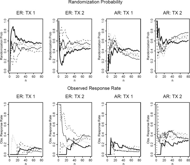
Randomization probability and observed response rate plotted over sequentially enrolled patients under the equal randomization (ER) and adaptive randomization (AR) designs. The probabilities of response in treatment 1 (TX1) and treatment 2(TX2) are 0.1 and 0.3, respectively. For the AR design, AR starts after the first 20 patients are equally randomized.

Table 1 shows the operating characteristics for four designs with 5,000 simulation studies using the Adaptive Randomization program developed at M. D. Anderson Cancer Center. (http://biostatistics.mdanderson.org/SoftwareDownload/). The four designs are (1) ER with N=200 without early stopping, (2) AR with N=200 without early stopping, (3) AR with N_max=200 and early stopping, and (4) AR with N_max=250 and early stopping. We evaluate the treatment effect by comparing the posterior distribution of the probability of response, e.g., treatment 1 is claimed to be better if Pr(p₁> p₂) > τ, where τ is an cutoff of the probability treatment 1 being better than treatment 2. An early stopping rule is implemented using cutoff of 0.999 and at the end of study a cutoff of 0.975 is used to make inference of the treatment efficacy. The performance of each method under the null hypothesis of p₁= p₂=0.3, and the alternative hypothesis of p₁=0.3, p₂=0.5 are studied. Without early stopping, ER yields 5% type I error rate and 83% power under the null and alternative hypotheses, respectively. With AR, the type I error rate is slightly higher (8%) and the power is a bit lower (75%) due to the imbalance of treatment assignment. Under H₁, the averaged numbers of patients randomized into treatment 1 and 2 are 46 and 154, respectively. The result illustrates the trade off between individual ethics and group ethics. AR enhances the individual ethics by assigning 77% of patients to the better treatment comparing to 50% by ER. However, due to imbalance in treatment allocation, the power is reduced from 83% to 75%.

Table 1.

Operating characteristics for two-arm Bayesian equal and adaptive randomization designs with and without early stopping. H₀: p₁= p₂= 0.3; H₁: p₁= 0.3, p₂= 0.5

	ER		AR		AR w/Early Stopping (Nmax=200)		AR w/Early Stopping (Nmax=250)
	H0	H1	H0	H1	H0	H1	H0	H1
N1	100	100	100	46	98	42	122	46
N2	100	100	100	154	97	125	121	150
N	200	200	200	200	195	167	243	196
P(declare TX1 better)	0.02	0	0.04	0	0.05	0	0.05	0
P(declare TX2 better)	0.03	0.83	0.04	0.75	0.05	0.76	0.05	0.85
P(early stopping)	0	0	0	0	0.04	0.34	0.04	0.44
P(randomized in arm 2)	0.50	0.50	0.50	0.77	0.50	0.75	0.50	0.77

One way to increase the study efficiency is to incorporate early stopping rules. Based on the interim result, if there is convincing evidence that one treatment is better than another, there is no need to continue the study. One can stop the trial early and announce the study result. Therefore, early stopping not only saves the sample size, but can also allow better treatment to be adopted earlier in the general population. With AR and early stopping, the type I error rate rises again slightly to 10%. There is a 4% chance of stopping the trial early under the null hypothesis. Under the alternative hypothesis, 34% of the time the trial will be stopped early. The averaged sample size is reduced from 200 to 167. The power and proportion of patients assigned to treatment 2 are comparable to AR without early stopping. To remedy the lower power resulting from imbalance due to AR, one can increase the maximum sample size. When the maximum sample size is increased to 250, the power is raised to 85%. The expected sample size is 196 with 77% of the patients receiving better treatment. Comparing to ER, the averaged number of patients treated in the trial is comparable. However, under the alternative hypothesis, AR with early stopping can result in both higher power and treating more patients with effective treatment, i.e., getting the best from both worlds. We can also add early futility stopping rules to further reduce the expected sample size under the null hypothesis.

Bayesian adaptive randomization and Frequentist’s designs applied in designs within two treatments, one marker

In the targeted agent development, putative markers play a role in guiding the selection of treatment. By convention, markers can be broadly classified as prognostic or predictive. A prognostic marker is a marker which is associated with the patient’s disease outcome regardless of treatment or in patients receiving standard care. For example, early stage patients tend to do better than late stage patients in cancer no matter what treatment is given. Patients with good performance status are likely to do better than patients with poor performance status, etc. In contrast, a predictive marker for a treatment is a marker which can predict the treatment outcome based on the marker status. For example, it is well established that lung cancer patients with EGFR mutation tend to do better than patients without mutation if they are given tyrosine kinase inhibitor such as gefinitib or erlotinib. The treatment does not work well in patients without mutation because they do not have the “target” for the targeted agent to work on. [27]

In the case with two treatments, one binary marker with a binary outcome, we illustrate that the Bayesian adaptive randomization (BAR) can be applied to achieve the following three goals: 1) test whether the marker is prognostic or predictive, 2) test whether the new treatment works better than the standard treatment in all patients or in patients within certain marker subsets, and 3) treat patients better in the trial by assigning more patients to the most effective treatment based on the patients’ marker status. Most of the standard frequentist designs can also achieved the first two goals.

Table 2 depicts five illustrative scenarios. Assume treatment 1 (TX1) is the standard treatment and treatment 2 (TX2) is a new targeted agent. All patients are evaluated for their marker status (− or +) before randomization. We assume that there are no measurement errors in marker status, and the outcome is binary and the result can be observed quickly. Scenario 1 shows the null case in which regardless of the patients’ marker status or the treatment assignment, the response rate (p) is 0.2 in all cases. Scenario 2 shows that the marker is prognostic where p = 0.4 in M+ patients, which is better than p = 0.2 in M− patients regardless of treatments. On the other hand, Scenario 3 shows the case where there is a treatment effect but no marker effect. Scenario 4 gives an example that the marker is predictive but not prognostic. The new treatment does not work in M− patients (p = 0.2), but works very well in M+ patients (p = 0.6). Lastly, Scenario 5 shows the case where the marker is both prognostic and predictive. Comparing to the standard treatment, the new treatment works slightly better in the M− patients but much better in M+ patients. (p = 0.2 vs. 0.1 and 0.6 vs. 0.3, respectively)

Table 2.

Response rates for two treatments and one marker in five scenarios.

	Scenario 1		Scenario 2		Scenario 3		Scenario 4		Scenario 5
	MK		MK		MK		MK		MK
TX	−	+	−	+	−	+	−	+	−	+
1	0.2	0.2	0.2	0.4	0.2	0.2	0.2	0.2	0.1	0.3
2	0.2	0.2	0.2	0.4	0.4	0.4	0.2	0.6	0.2	0.6

Several designs have been proposed in the literature for evaluating targeted agent in this setting. We compare the operating characteristics of five recently proposed designs, namely, the simple randomization design, the marker stratified design, the marker strategy design, [28] the efficient targeted design [24–25] and the Bayesian adaptive randomization design. The schematic diagram of these designs is given in Figure 2. In the simple randomization design, patients are randomized equally into the standard or the targeted treatment without the knowledge of the marker status. Simple randomization design can be used to test the overall treatment effect in the whole patient population. Conditional on the post-hoc analysis by patients’ marker status, it can also be used to test treatment effect in the M− and M+ patients separately. However, the marker distribution may not be balanced between the two treatment groups for small samples. If markers are measured retrospectively, a higher missing rate could occur. On the other hand, the marker stratified design requires that marker values be obtained at baseline. Upon stratifying on marker status, patients are equally randomization into the standard and targeted treatments. The prognostic effect of the marker can be tested by comparing A vs. C. Testing A vs. B or C vs. D can be used to assess the treatment effects in patients within each marker group. The predictive effect can be tested by comparing the odds of treatment response between M− and M+ patients (A/B vs. C/D). In the marker strategy design, patients are first randomized between strategies. Patients randomized into the non-strategy arm either receive the standard treatment, or can be randomized equally to the standard and targeted treatments. The latter design is used for comparing with other designs. For patients randomized into the marker-strategy arm, the treatment assignment is deterministic. M− patients receive standard treatment while M+ patients receive targeted treatment. The differential effect of the two strategies can be compared by testing A+B vs. C+D. The comparison between A and B can test the treatment effect in the unselected population. Similarly, the treatment effect in the selected population can be tested by the comparison between C and D. Efficient targeted design is an enrichment design which only treats M+ patients in the trial. M− patients are treated off protocol. It can answer the question whether targeted treatment works in the M+ patients, but its effectiveness in M− patients cannot be assessed.

Figure 2.

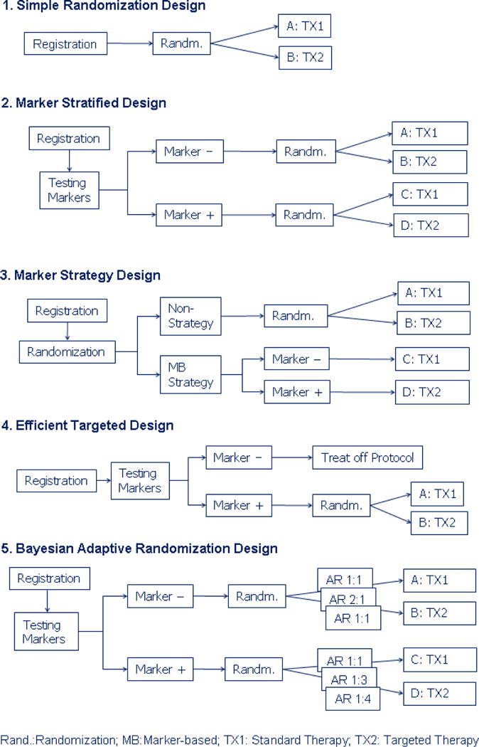
Schematic diagram for the five designs for the development of targeted agents.

BAR design is a model based approach, where the treatment effects are evaluated in marker groups progressively. The design structure is similar to marker stratified design, where randomization is conducted conditionally on marker status. However, instead of using ER, covariate-adjusted AR by marker is applied to allocate more patients to the putatively superior treatment.

With two marker groups and two treatments, logistic regression can be applied to test for the marker effect, the treatment effect, and their interaction. The model can be formulated as follows. For patient i, we assume

$$\begin{array}{l}\text{Pr}\left(Y_i=1\right)={\theta }_i\\ \text{log}\left(\frac{{\theta }_i}{1-{\theta }_i}\right)={\beta }_0+{\beta }_M{M}_i+{\beta }_T{T}_i+{\beta }_I{M}_i\cdot T_i\end{array}$$ (1)

, where Y_i is the response indicator, θ_i is the probability of response, M_i is the marker indicator and T_i is the treatment indicator. For the BAR design, we assume that the parameters follow a multivariate normal distribution with a non-informative prior. Simulation studies are performed to evaluate the operating characteristics of the above designs. We run 5,000 simulations for the frequentist designs and 1,000 simulations for the Bayesian design. We assume that the total sample size is 150 and the M+ probability of 0.5. Table 3 gives the statistical power for testing the marker effect, the treatment effect, and the marker by treatment interaction (i.e., whether the marker is predictive). For the marker strategy design, since patients’ marker status is assumed to be available, we carry out the post-hoc logistic regression analysis to test for the above effects. In addition, we report the results of testing whether the treatment works in patients randomized into non-strategy and strategy approaches, and the power for comparing the two strategies. The last column shows the averaged overall response rate in all patients enrolled in the trial. All the frequentist tests are carried out at a two-sided 5% significance level.

Table 3.

Operating characteristics for five designs in testing the marker effect, treatment effect, and marker by treatment interaction (marker predictive effect). The statistical power and overall response rate are shown in five scenarios.

Scenario	Design	Marker Effect			Treatment Effect						MK × Interaction**	Overall Resp. Rate
		In TX1*	In TX2	Overall	In MK(−)	In MK(+)	Overall	In STR(−)	In STR(+)	STR(−) vs STR(+)
1	Simple Rand.	0.04	0.02	0.06	0.04	0.02	0.06				0.05	0.20
	Marker Stratified	0.04	0.02	0.06	0.03	0.02	0.06				0.05	0.20
	Marker Strategy	0.03	0.00	0.03	0.03	0.00	0.03	0.05	0.05	0.05	0.03	0.20
	Efficient Target					0.04						0.20
	Bayesian AR	0.03	0.02	0.05	0.02	0.04	0.06				0.03	0.20
2	Simple Rand.	0.46	0.45	0.71	0.04	0.02	0.06				0.05	0.30
	Marker Stratified	0.47	0.47	0.72	0.03	0.03	0.06				0.05	0.30
	Marker Strategy	0.40	0.28	0.56	0.03	0.02	0.04	0.06	0.46	0.05	0.04	0.30
	Efficient Target					0.05	0.05					0.40
	Bayesian AR	0.46	0.43	0.71	0.02	0.03	0.05				0.04	0.30
3	Simple Rand.	0.04	0.02	0.06	0.46	0.45	0.70				0.05	0.30
	Marker Stratified	0.04	0.02	0.06	0.46	0.47	0.72				0.04	0.30
	Marker Strategy	0.03	0.02	0.05	0.38	0.25	0.54	0.46	0.46	0.05	0.04	0.30
	Efficient Target					0.47						0.30
	Bayesian AR	0.02	0.03	0.05	0.36	0.38	0.62				0.02	0.34
4	Simple Rand.	0.04	0.95	0.95	0.04	0.95	0.95				0.64	0.30
	Marker Stratified	0.04	0.95	0.95	0.03	0.94	0.95				0.62	0.30
	Marker Strategy	0.03	0.86	0.86	0.03	0.84	0.84	0.46	0.95	0.25	0.46	0.35
	Efficient Target					0.95						0.40
	Bayesian AR	0.02	0.98	0.98	0.04	0.87	0.87				0.50	0.35
5	Simple Rand.	0.54	0.95	0.98	0.15	0.75	0.79				0.08	0.30
	Marker Stratified	0.54	0.95	0.98	0.15	0.74	0.78				0.08	0.30
	Marker Strategy	0.52	0.86	0.93	0.19	0.60	0.66	0.46	1.00	0.10	0.05	0.33
	Efficient Target					0.75						0.45
	Bayesian AR	0.40	0.98	0.99	0.19	0.66	0.71				0.06	0.34

^*: Testing whether marker is prognostic.

^**: Testing whether marker is predictive.

TX: Treatment; MK: Marker: STR: Strategy; Overall Resp. Rate: overall response rate.

For the BAR design, we let the first 50 patients to be equally randomized so we can obtain initial estimates of the parameters. Starting from the 51st patient, patients are randomized to treatment 1 with probability ${\widehat{p}}_1/({\widehat{p}}_1+{\widehat{p}}_2)$ where ${\widehat{p}}_i$ is the current estimate of the response rate in treatment i, i=1, 2. At the end of study, a parameter β is considered significantly different from 0 if Prob(β>0) >τ, where β represents for β_T in testing treatment effect in M− patients, for β_T + β_I in testing treatment effect in M+ patients, for β_M in testing marker effect in TX1, and for β_M + β_I in testing marker effect in TX2. An overall treatment effect is defined as TX2 is better either M− or M+ patients. Similar definition is applied for the overall marker effect. The cutoff, τ is selected to correspond to 5% type I error rate under the null hypothesis.

In Scenario 1, when there is no marker effect nor treatment effect, the statistical power (type I error) is between 0 and 0.06 in all settings. The overall response rate is indeed 0.2 in all settings. In our case with the M+ proportion being 0.5, the performance of the simple randomization design and the marker stratified design (both are ER designs) is essentially identical.

For Scenario 2, ER design shows the power for testing the marker effect is about 46% in each treatment subgroups and about 71% in all patients. Due to the imbalanced allocation in the marker strategy design (approximately 37.5% in the M−, TX1 and M+, TX2 and 12.5% in M−,TX2 and M+, TX1), the corresponding powers are reduced. Since there is no treatment effect, the powers for testing the treatment effect are around the levels of type I error rates of null case in all designs.

In scenario 3, when there is a treatment effect but no marker effect, all designs show the power for testing the marker effect is hovering around the 5% type I error rate. The power for testing the overall treatment effect is higher in the ER design (about 71%) than the marker strategy design (54%) as shown earlier. The power for testing the treatment effect using the efficient targeted design is only 47% because it screens out the M− patients.

In Scenario 4, when marker is predictive but not prognostic, the type I errors for testing the marker’s prognostic effect and the treatment effect in M− patients are all less than 5% for all designs. The power for testing the marker effect in TX2 patients or treatment effect in M+ patients are greater than 90% for the ER design and the efficient targeted design but in the mid-80% range for the marker strategy design. The power for testing the marker’s predictive effect (i.e., marker by treatment interaction) is about 63% for the ER designs and only 46% for the marker strategy design.

In Scenario 5, when the marker is both prognostic and predictive, the powers for testing the marker effect and the treatment effect are all greater than the nominal significance level. The performance of the efficient targeted design is similar to the ER designs and is better than the marker strategy design.

For the marker strategy design, we also evaluate the treatment effect in patients assigned to non-strategy arm, strategy arm, and the power for comparing strategy versus non-strategy arm. For Scenario 2, the power for testing the treatment effect in patients assigned to the strategy approach arm is 46%. This means that taking the marker strategy approach, patients assigned to the targeted agent fare better when patients are assigned to the standard treatment. Hence, it may lead to an erroneous conclusion that the targeted agent works better than the standard treatment. The difference is, in fact, due to the marker effect and not the treatment effect. The strategy approach leads to a total confounding between marker and treatment. Hence, when difference is observed, it is not known whether it is attributed to the marker or the treatment. One other important observation is that, for the marker strategy design, the power for testing strategy versus no-strategy approaches is consistently low in all scenarios. Even in Scenarios 4 and 5, when the marker is predictive, the powers are only 25% and 10%, respectively. The low power is a result of a significant overlap in treatment assignments between the two.

For the BAR design, we choose the cutoff value τ = 0.983 to control the type I error rate to 0.05. For Scenario 2, the powers of the BAR design for testing the marker effect are comparable to the ER design. For Scenario 3, the power of the BAR design for testing the treatment effect is slightly lower than the ER design (62% versus 70% for testing overall treatment effect). Due to AR, the slight loss of power can also be seen in Scenarios 4 and 5 (87% versus 95% and 71% versus 79%, respectively).

We also compare the overall response rate in all designs. For Scenario 2, efficient targeted design has 40% response rate because only M+ patients are enrolled. In Scenario 3, BAR gave the best result with a response rate of 34%. For Scenario 4, efficient targeted design yields a response rate of 40% while the marker strategy design and BAR give a response rate of 35%. Likewise, in Scenario 5, efficient targeted design has the highest overall response rate (45%), followed by BAR (34%), marker strategy design (33%), and ER (30%). ER design has the lowest response rate in all scenarios.

Bayesian adaptive randomization applied in designs with multiple treatments and multiple markers

Bayesian adaptive randomization design can be applied to settings when multiple markers are involved in evaluating the effect of multiple treatments. To illustrate its use, we give an example when two markers are used for evaluating four treatments. Specifically, we recently designed a biomarker-based clinical trial in advanced staged lung cancer patients. Building upon a similar trial called BATTLE (Biomarker-integrated approaches of targeted therapy of lung cancer elimination),[28] our BATTLE-2 trial is to test four treatments with multiple biomarkers. The primary endpoint is the 8-week disease control rate (DCR) defined as patients without progression by the end of 8 weeks after randomization.[29] The trial was designed with a total sample size of 320 in two stages (160 patients per stage). There are four treatments, namely, erlotinib, erlotinib + an AKT inhibitor, erlotinib + an IGFR-inhibitor, and an AKT-inhibitor + a MEK-inhibitor. In stage 1, two well established markers (EGFR mutation and K-ras mutation) are used to guide the patient allocation. Patients will be adaptively randomized in stage 1 based on the two markers. From stage 1, more putative and discovery markers are identified to refine the predictive model which will then be used in adaptively randomizing patients in stage 2.

We use only the stage 1 part to illustrate how BAR can be applied in this setting. The design has one more complication: two types of patients are recruited – erlotinib naïve who have not been exposed with erlotinib and erlotinib resistant who had prior erlotinib treatment but failed. Per design, erlotinib naïve patients can be randomized in any one of the four treatments but erlotinib resistant patients can only be randomized into one of the three combination treatments.

The statistical model is given below. Let X_i be a n×q design matrix, n = total numbers of patients, q = total numbers of parameter including intercept, J = total number of treatments, and K = total number of markers. Under the framework of the logistic model, the disease control rate p_i for the ith patient can be expressed as

$$\begin{array}{l}\text{logit}\left(p_i\right)=X_i\beta ={\alpha }_1+{\displaystyle \sum _{j=2}^J{\alpha }_j{T}_{ij}+{\displaystyle \sum _{k=1}^K{\beta }_k{M}_{ik}+{\displaystyle \sum _{j=2}^J{\displaystyle \sum _{k=1}^K{\gamma }_{kj}{M}_{ik}{T}_{ij}}}}}\\ +\left({{\alpha }_1}^{\prime }+{\displaystyle \sum _{j=2}^J{{\alpha }_j}^{\prime }{T}_{ij}+{\displaystyle \sum _{k=1}^K{{\beta }_k}^{\prime }{M}_{ik}+{\displaystyle \sum _{j=2}^J{\displaystyle \sum _{k=1}^K{{\gamma }_{kj}}^{\prime }{M}_{ik}}{T}_{ij}}}}\right)\cdot Z_i\end{array}$$ (2)

where T_ij is the indicator for the experimental treatments (TX2, TX3, or TX4), M_ik is the indicator for positive marker status, and Z_i is the indicator for erlotinib-resistant patient.

For erlotinib-naïve patients, the probability of patient being assigned to the jth treatment is proportional to $\text{Pr}(p_j>p_{j\prime },j\prime \in \{1,2,3,4|j\prime \ne j\})$. For erlotinib-resistant patients, allocation to TX1 is prohibited, and the probability of patient being assigned to TX2, TX3, or TX4 is proportional to $\text{Pr}(p_j>p_{j\prime },j\prime \in \{2,3,4|j\prime \ne j\})$.

Our main interest is to test for the effect of new treatments (TX2, 3, 4) versus the standard treatment (TX1) in the following settings.

1. Evaluation of the marginal treatment effect in all patients

The marginal treatment effect will be tested using model (3) with only treatment and marker main effect present.

$$\text{logit}\left(p_i\right)+{\alpha }_1+{\alpha }_2{T}_{i2}+{\alpha }_3{T}_{i3}+{\alpha }_4{T}_{i4}+{\beta }_1{M}_{i1}+{\beta }_2{M}_{i2}$$ (3)

Experimental treatment, TX j (j =2, 3, 4) will be claimed as having a significant marginal treatment effect in all patients if Pr(α_j > 0) >τ, where τ is the threshold cutoff value for posterior inference. That is, we call the experimental treatment better than the standard if the probability of the DCR in the experimental treatment being greater than the DCR in the standard treatment is greater than τ.

2. Evaluation of the marginal treatment effect in erlotinib resistant and in erlotinib naïve patients

The marginal treatment effect in the erlotinib resistant and in the erlotinib naïve patients will be tested using model (4) which including Z_i.

$$\begin{array}{l}\text{logit}\left(p_i\right)={\alpha }_1+{\alpha }_2{T}_{i2}+{\alpha }_3{T}_{i3}+{\alpha }_4{T}_{i4}+{\beta }_1{M}_{i1}+{\beta }_2{M}_{i2}\\ +\left({{\alpha }^{\prime }}_1+{{\alpha }^{\prime }}_2{T}_{i2}+{{\alpha }^{\prime }}_3{T}_{i3}+{{\alpha }^{\prime }}_4{T}_{i4}+{{\beta }^{\prime }}_1{M}_{i1}+{{\beta }^{\prime }}_2{M}_{i2}\right)\cdot Z_i\end{array}$$ (4)

TX j (j =2, 3, 4) will be claimed as having a significant marginal treatment effect in naïve patients if Pr(α_j > 0) >τ and in resistant patients if $\text{Pr}({\alpha }_j+{{\alpha }^{\prime }}_j>0)>\tau$.

3. Evaluation of the treatment effects in erlotinib resistant and in erlotinib naïve patients in different marker groups

It is assume that, among erlotinib-naïve patients, M1+ patients will have a better response to the experimental treatments than M1− patients. If there are no marginal treatment effects in either the overall patient population or erlotinib naïve or resistant patients, we will further evaluate the treatment effect in erlotinib naive patients expressing particular markers using the full model in equation (2).

Experimental treatment j (j =2, 3, 4) will be claimed as having a significant treatment effect in erlotinib naïve and marker k positive patients if Pr(α_j +γ_kj > 0) >τ and in erlotinib resistant and marker k positive patients if $\text{Pr}({\alpha }_j+{\gamma }_{kj}+{\alpha }_j^{\prime }+{\gamma }_{kj}^{\prime }>0)>\tau$.

Simulations are conducted with 2000 runs for each scenario to evaluate the operating characteristics. For each run, a total of 5000 Markov chain Monte Carlo (MCMC) iterations after 5000 burn-in draws are used to make posterior inferences. We assume 44% of the 160 patients are erlotinib resistant and the remaining 56% are erlotinib naïve based on our prior data. We also assume that the EGFR mutation rate and K-ras mutation rate are both at 20% and they are independent to each other. Two priors were used to evaluate the operating characteristics: 1) A non-informative (NI) independent Normal (0,100) prior is used for all parameters; 2) Same as in 1) but an informative beta prior for the erlotinib only treatment in the erlotinib resistant patients. Since no erlotinib resistant patients are assigned to the erlotinib only arm, when testing the treatment efficacy in resistant patients with the NI prior option, the inference is essentially based on comparing the treatment effects of experimental arms to a very diffuse prior centered at 0.5, which could yield a very low power. Therefore, the use of a non-informative prior may not be reasonable. The very reason that we do not assign erlotinib resistant patients into the erlotinib only arm is because the treatment does not work in this setting. Sim et al. (30) reported data from 16 patients who were treated with gefitinib first, followed by erlotinib upon gefitinib failure. The disease control rate was 69% in the gefitinib treatment and 25% in the subsequent erlotinib treatment. We implement this information through our second prior option, the beta prior. To discount the weight of the historical data, we assume that the DCRs for the erlotinib treatment in the erlotinib resistant patients follow beta prior distributions with an effective sample size of 5 and the mean corresponding to each of the marker groups in Table 4, our assumed treatment effect in the simulation. The order of magnitude of treatment effect in the literature is similar to that is shown in Table 4.

Table 4.

Assumed 8-week disease control rate under the null and alternative hypotheses for erlotinib resistant and naïve patients by marker status in the BATTLE-2 design

Under Null Hypothesis
Markers		Erlotinib Naïve				Erlotinib Resistant
M1	M2	TX1	TX2	TX3	TX4	TX2	TX3	TX4
−	−	0.3	0.3	0.3	0.3	0.1	0.1	0.1
+	−	0.6	0.6	0.6	0.4	0.2	0.2	0.1
−	+	0.1	0.1	0.1	0.1	0.1	0.1	0.1
Under Alternative Hypothesis
Markers		Erlotinib Naïve				Erlotinib Resistant
M1	M2	TX1	TX2	TX3	TX4	TX2	TX3	TX4
−	−	0.3	0.6	0.6	0.6	0.5	0.5	0.5
+	−	0.6	0.9	0.9	0.7	0.6	0.6	0.6
−	+	0.1	0.3	0.3	0.5	0.3	0.3	0.5

The total numbers of patients randomized into each marker by treatment combinations are given in Table 5. Under the null hypothesis, the numbers of patients treated in each arm are very similar to each other as expected. Under the alternative hypothesis, for naïve patients, the numbers of patients in the erlotinib arm is smaller than the combination arms because the combination arms have higher DCRs.

Table 5.

Observed averaged number of patients under the null and alternative hypotheses for erlotinib resistant and naïve patients by marker status in the BATTLE-2 design

Under Null Hypothesis
Markers		Erlotinib Naïve				Erlotinib Resistant
M1	M2	TX1	TX2	TX3	TX4	TX2	TX3	TX4
−	−	15.2	14.0	14.5	13.3	14.9	15.6	14.6
+	−	3.9	3.9	3.3	3.4	3.7	3.5	4.1
−	+	2.9	5.1	3.6	2.8	4.5	3.7	2.9
+	+	0.8	1.1	0.8	0.8	1.0	0.9	0.9
Under Alternative Hypothesis
Markers		Erlotinib Naïve				Erlotinib Resistant
M1	M2	TX1	TX2	TX3	TX4	TX2	TX3	TX4
−	−	10.0	15.9	15.9	15.7	14.8	14.8	15.4
+	−	3.3	4.1	3.6	3.4	4.0	3.8	3.5
−	+	2.1	4.9	3.3	4.0	3.9	3.2	4.0
+	+	0.7	1.1	0.8	0.9	1.0	0.9	0.9

Table 6 shows the statistical power for testing the treatment effect under various settings. A significant overall treatment effect is defined as significant if the effect is shown in either marginal effect (for all patients or for subgroup of patients) or in any marker positive patients. If any of TX 2, 3, and 4 have significant effect, the trial will be claimed as a success. For the Bayesian design, a cutoff value τ, is chosen to declare the test result being “significant”. We chose τ such that the type I error rate under the null hypothesis for testing treatment effect of experimental arm versus erlotinib only arm is 10%. For noninformative prior, τ=0.982 and for the beta prior, τ=0.984.

Table 6.

Statistical power for testing the treatment effect under the null and alternative hypotheses for erlotinib resistant and naïve patients by marker status in the BATTLE-2 adaptive randomization design using the Bayesian logistic regression. Cut-off values for posterior probability were chosen to control the type I error rates for comparing TX 2, 3, 4 to TX 1 under the null hypothesis to 10%.

Prior	Scenario	Cut-off	TX	Margin	Naïve. Margin	Resist. Margin	Naïve. MK(−,−)	Naïve. MK(+,−)	Naïve. MK(−,+)	Resist. MK(−,−)	Resist. MK(+,−)	Resist. MK(−,+)	Overall	All TX
NI	Null	0.982	2	0.004	0.040	0.000	0.035	0.046	0.014	0.000	0.000	0.000	0.098	0.184
			3	0.004	0.034	0.000	0.034	0.052	0.011	0.001	0.001	0.001	0.093
			4	0.004	0.018	0.000	0.033	0.010	0.002	0.000	0.000	0.000	0.044
	Alt.		2	0.302	0.463	0.003	0.348	0.293	0.083	0.004	0.004	0.000	0.632	0.865
			3	0.316	0.442	0.001	0.358	0.263	0.098	0.003	0.009	0.000	0.592
			4	0.375	0.440	0.002	0.348	0.102	0.244	0.003	0.004	0.011	0.622
Beta5	Null	0.984	2	0.003	0.038	0.000	0.033	0.041	0.013	0.000	0.001	0.000	0.091	0.174
			3	0.003	0.033	0.010	0.030	0.049	0.009	0.000	0.001	0.001	0.095
			4	0.004	0.016	0.000	0.030	0.009	0.001	0.000	0.000	0.001	0.039
	Alt.		2	0.291	0.447	0.277	0.336	0.277	0.071	0.271	0.211	0.039	0.787	0.987
			3	0.299	0.432	0.579	0.338	0.243	0.087	0.299	0.230	0.050	0.861
			4	0.357	0.423	0.040	0.337	0.096	0.225	0.311	0.208	0.207	0.801

With the noninformative prior, the powers for testing TX2, 3, and 4 being better than TX1 are 0.632, 0.592, and 0.622, respectively. The power gains are mainly from the erlotinib naïve patients as it is evident that the power gain from the erlotinib resistant patients is essentially nil. This is due to the nature of the noninformative prior and no resistant patients is assigned to the erlotinib only arm to update information. In contrast, even with a weak informative beta prior (with an effective sample size of 5), we gain power for testing the treatment effect in the resistant patients. The power for testing TX 2, 3, and 4 being effective increased to 0.787, 0.861, and 0.801, respectively. The overall family-wise type I error rate is 0.184 and 0.174 for the non-informative and beta prior respectively. The corresponding overall power is 0.865 and 0.987.

To compare the performance of the Bayesian design with frequentist’s design, Table 7 shows the corresponding statistical power using the Fisher’s exact test. Because there is no data in the erlotinib resistant group treated with erlotinib, we show the results based on the whole group (margin) and for the naïve patients only. Fisher’s exact test is chosen because the maximum likelihood estimators from logistic regressions often failed due to the small sample size and no events in biomarker subgroups. The overall power is 0.923 which is higher than the Bayesian design with a non-informative prior but lower than the Bayesian design with an informative prior.

Table 7.

Statistical power for testing the treatment effect under the null and alternative hypotheses for all patients and for erlotinib naïve patients by marker status in the frequentist’s equal randomization design. A p-value cut-off of 0.108 for the Fisher’s exact test was chosen to control the type I error rates for comparing TX 2, 3, 4 to TX 1 under the null hypothesis to 10%.

Scenario	TX	Margin	Naïve Margin	Naïve MK(−,−)	Naïve MK(+,−)	Naïve MK(−,+)	Overall	All TX
Null	2	0.007	0.054	0.044	0.018	0.003	0.097	0.200
	3	0.006	0.058	0.053	0.018	0.001	0.099
	4	0.004	0.036	0.050	0.004	0.001	0.071
Alt.	2	0.579	0.644	0.487	0.076	0.031	0.741	0.923
	3	0.593	0.651	0.495	0.081	0.035	0.756
	4	0.639	0.650	0.495	0.021	0.135	0.758

Discussion

For developing targeted agents, it is indeed challenging to ask for a design which is accurate, efficient, ethical, and flexible. Through simulation studies, we have compared the performance of various frequentist designs and the Bayesian adaptive randomization design. For the frequentist designs, simple randomization design and marker stratified design have similar operating characteristics, but the marker stratified design can ensure that treatments are equally assigned in each marker group, and the prospective evaluation of markers can improve the completeness and accuracy of the marker data. Efficient targeted design only tests the treatment efficacy in selected marker group(s), hence, it reduces the trial sample size. It is most efficient when there is sufficient evidence that the treatment is most likely to work only in the selected marker groups and unlikely to work in the other groups. However, in most settings, the answers to these questions remain unknown. This is the exact reason why we need to conduct clinical trials in the first place. Although the efficient targeted design can test the treatment effect in the selected group, the effect in other marker groups cannot be assessed. Marker strategy design may sound like a reasonable approach but due to the confounding between the marker effect and the treatment effect, the design cannot accurately attribute the difference in outcomes to marker, treatment, or their combinations. The design also has very little power in comparing the strategy versus non-strategy approaches.

Bayesian adaptive randomization design allocates more patients in more effective treatments as the trial progresses and information accumulates. It continues to learn about the effects of markers, treatments, and their interactions along the trial and adjusts the randomization proportion accordingly. By carefully calibrating the design parameters, type I and type II errors can be controlled for the Bayesian designs. AR can result in mild loss in statistical power due to imbalance allocation between treatment groups. It, however, gains efficiency through modeling and the appropriate use of the prior information. Furthermore, adding futility or efficacy early stopping rules can reduce the sample size. Although the BAR designs yield only incremental improvements over the frequentist’s counterparts, Bayesian approach provides a uniform way of setting up complex problems, parameter estimation, and inference making. Bayesian framework also allows more flexible study conduct, such as dropping ineffective treatments and adding new treatments, because the inference is based on the data (conformed with the likelihood principle) and does not depend on a fixed sampling plan.

The validity of the Bayesian models we have discussed, however, depends on the proper model specification and the assumed parameters. Extensive simulations should be conducted to evaluate the operating characteristics of the design under various settings. A conservative approach should be taken in choosing the sample size and in controlling type I errors. Highly complex models may gain efficiency but lack robustness. Model checking and sensitivity analysis are required to ensure that the model provides adequate fit for the data.

Early phase of drug developing is about discovery and learning. Adaptive design provides an ideal platform for learning and enables the investigators to continue to learn about the new agents’ clinical activities during the trial and apply this knowledge to better treat patients in real time. It can increase the study efficiency, allow flexibility in study conduct, and provide better treatment to study participants, which is a step towards personalized medicine. One limitation of the response adaptive randomization is that it requires that the response to be assessed in a relatively short time period. Infrastructure setup needs to allow more frequent monitoring of interim results. Extra steps need to be taken to ensure the integrity of the study conduct, e.g., timely and objective evaluation of endpoints. Due to the large number of tests, the overall false positive rate may increase. Results found in one trial need to be confirmed in other trials, which includes the validation of both the predictive markers and the treatment efficacy. Upon the identification of efficacious treatments and corresponding markers, a more focused confirmatory trial can be designed accordingly.

The success of Bayesian adaptive trials requires an integrated multi-disciplinary research team of clinical investigators, who see patients and perform biopsies, basic scientists who run the biomarker analysis, computer programmers who build web-based database applications, and statisticians who provide the design and implement adaptive randomization.

In summary, Bayesian designs can be more ethical and efficient by incorporating adaptive randomization and early stopping rules. The proposed new designs incorporate rational learning from the interim data for randomization and making decisions on treatment efficacy. Bayesian adaptive randomization designs are distinctively suitable for the development of multiple targeted agents with multiple biomarkers. Although it requires more efforts on trial design, simulation, setting up the infrastructure, trial conduct, analysis, and reporting, Bayesian designs have gain increasing popularity recently and have been implemented in many settings.[23, 28] In reviewing papers demonstrating that Bayesian clinical trials are currently in action, Gonen has aptly titled his editorial: “Bayesian clinical trials: no more excuses.”[31]

References

- 1.Kummar S, Gutierrez M, Doroshow JH, Murgo AJ. Drug development in oncology: classical cytotoxics and molecularly targeted agents. Br J Clin Pharmacol. 2006;62:15–26. doi: 10.1111/j.1365-2125.2006.02713.x. [DOI] [PMC free article] [PubMed] [Google Scholar]
- 2.O’Hare T, Deininger MW. Toward a cure for chronic myeloid leukemia. Clin Cancer Res. 2008;14(24):7971–7974. doi: 10.1158/1078-0432.CCR-08-1486. [DOI] [PMC free article] [PubMed] [Google Scholar]
- 3.Buzdar AU. Role of biologic therapy and chemotherapy in hormone receptor- and HER2-positive breast cancer. Ann Oncol. 2009;20(6):993–999. doi: 10.1093/annonc/mdn739. [DOI] [PubMed] [Google Scholar]
- 4.Chackalamannil S, Desai MC. Personalized medicine - A paradigm for a sustainable pharmaceutical industry? Curr Opin Drug Discov Devel. 2009;12(4):443–445. [PubMed] [Google Scholar]
- 5.Fine BM, Amler L. Predictive biomarkers in the development of oncology drugs: A therapeutic industry perspective. Clin Pharmacol Ther. 2009;85(5):535–538. doi: 10.1038/clpt.2009.9. [DOI] [PubMed] [Google Scholar]
- 6.Tepper RI, Roubenoff R. The role of genomics and genetics in drug discovery and development. In: Willard HF, Ginburg GS, editors. Genomic and Personalized Medicine. Academic Press; San Diego, CA, USA: 2009. pp. 335–356. [Google Scholar]
- 7.Cooley ME, Sarna L, Brown JK, et al. Challenges of recruitment and retention in multisite clinical research. Cancer Nurs. 2003;26(5):376–386. doi: 10.1097/00002820-200310000-00006. [DOI] [PubMed] [Google Scholar]
- 8.Rosenberger WF, Lachin JM. Randomization in Clinical Trials: Theory and Practice. Wiley; New York: 2002. [Google Scholar]
- 9.Hu F, Rosenberger WF. Optimality, Variability, Power: Evaluating Response-Adaptive Randomization Procedures for Treatment Comparisons. J Am Stat Assoc. 2003;98:671–678. [Google Scholar]
- 10.Hu F, Rosenberger WF. The Theory of Response-adaptive Randomization in Clinical Trials. Wiley; Hoboken, New Jersey: 2006. [Google Scholar]
- 11.Thall PF. Ethical issues in oncology biostatistics. Stat Methods Med Res. 2002;11:429–448. doi: 10.1191/0962280202sm301ra. [DOI] [PubMed] [Google Scholar]
- 12.Berry DA. Bayesian statistics and the efficiency and ethics of clinical trials. Stat Sci. 2004;19:175–187. [Google Scholar]
- 13.Show S-C, Chang M. Adaptive Design Methods in Clinical Trials. Chapman and Hall/CRC; Boca Raton, Florida: 2007. [Google Scholar]
- 14.Chang M. Adaptive Design Theory and Implementation Using SAS and R. Chapman and Hall/CRC; Boca Raton, Florida: 2008. [Google Scholar]
- 15.Berry DA. Adaptive trial design. Clin Adv Hematol Oncol. 2007;5(7):522–524. [PubMed] [Google Scholar]
- 16.Biswas A. Adaptive designs for binary treatment responses in phase III clinical trials: controversies and progress. Stat Methods Med Res. 2001;10:353–364. doi: 10.1177/096228020101000504. [DOI] [PubMed] [Google Scholar]
- 17.Biswas S, Liu DD, Lee JJ, Berry DA. Bayesian clinical trials at the University of Texas M. D. Anderson Cancer Center. Clin Trials. 2009;6:205–216. doi: 10.1177/1740774509104992. [DOI] [PMC free article] [PubMed] [Google Scholar]
- 18.Goodman SN. Introduction to Bayesian methods I: Measuring the strength of evidence. Clin Trials. 2005;2:282–290. doi: 10.1191/1740774505cn098oa. [DOI] [PubMed] [Google Scholar]
- 19.Louis TA. Introduction to Bayesian methods II: Fundamental concepts. Clin Trials. 2005;2:291–294. doi: 10.1191/1740774505cn099oa. [DOI] [PubMed] [Google Scholar]
- 20.Berry DA. Introduction to Bayesian methods III: Use and interpretation of Bayesian tools in design and analysis. Clin Trials. 2005;2:295–300. doi: 10.1191/1740774505cn100oa. [DOI] [PubMed] [Google Scholar]
- 21.Spiegelhalter DJ, Abrams KR, Myles JP. Bayesian Approaches to Clinical Trials and Health-Care Evaluation. John Wiley & Sons; Chichester, West Sussex, UK: 2004. [Google Scholar]
- 22.Berry DA. A guide to drug discovery: Bayesian clinical trials. Nat Rev Drug Discov. 2006;5:27–36. doi: 10.1038/nrd1927. [DOI] [PubMed] [Google Scholar]
- 23.Berry DA. Statistical innovations in cancer research. In: Holland J, Frei T, et al., editors. Cancer Medicine. 7th. Decker BC; London: 2005. pp. 411–425. [Google Scholar]
- 24.Simon R, Maitournam A. Perspective evaluating the efficiency of targeted designs for randomized clinical trials. Clin Can Res. 2004;10:6759–6763. doi: 10.1158/1078-0432.CCR-04-0496. [DOI] [PubMed] [Google Scholar]
- 25.Maitournam A, Simon R. On the efficiency of targeted clinical trials. Stat Med. 2005;24:329–339. doi: 10.1002/sim.1975. [DOI] [PubMed] [Google Scholar]
- 26.Sargent DJ, Conley BA, Allegra C, Collette L. Clinical trial designs for predictive marker validation in cancer treatment trials. J Clin Oncol. 2005;23:2020–2027. doi: 10.1200/JCO.2005.01.112. [DOI] [PubMed] [Google Scholar]
- 27.Dahabreh IJ, Linardou H, Siannis F, Kosmidis P, Bafaloukos D, Murray S. Somatic EGFR mutation and gene copy gain as predictive biomarkers for response to tyrosine kinase inhibitors in non-small cell lung cancer. Clinical Cancer Research. 2010;16:291–303. doi: 10.1158/1078-0432.CCR-09-1660. [DOI] [PubMed] [Google Scholar]
- 28.Zhou X, Liu S, Kim ES, Herbst RS, Lee JJ. Bayesian adaptive design for targeted therapy development in lung cancer - A step toward personalized medicine. Clin Trials. 2008;5:181–193. doi: 10.1177/1740774508091815. [DOI] [PMC free article] [PubMed] [Google Scholar]
- 29.Lara PN, Jr, Redman MW, Kelly K, et al. Disease control rate at 8 weeks predicts clinical benefit in advanced non-small-cell lung cancer: Results from Southwest Oncology Group randomized trials. J Clin Oncol. 2008;26:463–467. doi: 10.1200/JCO.2007.13.0344. [DOI] [PubMed] [Google Scholar]
- 30.Sim SH, Han S-W, Oh D-Y, et al. Erlotinib after Gefitinib failure in female never-smoker Asian patients with pulmonary adenocarcinoma. Lung Cancer. 2009;65:204–207. doi: 10.1016/j.lungcan.2008.11.006. [DOI] [PubMed] [Google Scholar]
- 31.Gönen M. Bayesian clinical trials: No more excuses. Clin Trials. 2009;6:203–204. doi: 10.1177/1740774509105374. [DOI] [PubMed] [Google Scholar]