

Abstract
Magnetic Particle Imaging (MPI) is an emerging tomographic imaging technology that detects magnetic nanoparticle tracers by exploiting their non-linear magnetization properties. In order to predict the behavior of nanoparticles in an imager, it is possible to use a non-imaging MPI relaxometer or spectrometer to characterize the behavior of nanoparticles in a controlled setting. In this paper we explore the use of ferrohydrodynamic magnetization equations for predicting the response of particles in an MPI relaxometer. These include a magnetization equation developed by Shliomis (Sh) which has a constant relaxation time and a magnetization equation which uses a field-dependent relaxation time developed by Martsenyuk, Raikher and Shliomis (MRSh). We compare the predictions from these models with measurements and with the predictions based on the Langevin function that assumes instantaneous magnetization response of the nanoparticles. The results show good qualitative and quantitative agreement between the ferrohydrodynamic models and the measurements without the use of fitting parameters and provide further evidence of the potential of ferrohydrodynamic modeling in MPI.
Keywords: Magnetic particle imaging (MPI), x-space MPI, ferrohydrodynamics, relaxation
1. Introduction
Magnetic Particle Imaging (MPI) [1] is capable of imaging biocompatible iron-oxide magnetic nanoparticle tracers with sub-millimeter resolution without using ionizing radiation. This technology exploits the non-linear magnetization response of the particles to obtain images where signal intensity is linearly proportional to nanoparticle concentration. Applications in real-time cardiovascular imaging [2] and cell tracking [3, 4] have been demonstrated and others are currently in development. There are currently two principal approaches to signal reconstruction used in MPI, based on System Function [1, 5] or x-space [6, 7] formulations, which have very different approaches to converting the signal generated by the nonlinear magnetization response of the nanoparticles into an image.
Goodwill and Conolly [6] introduced the use of an x-space relaxometer to characterize the behavior of nanoparticles in MPI scanners based on the x-space reconstruction formulation. The instrument consists of a set of concentric solenoid coils. The outermost coil, called the bias coil, delivers a ramping DC magnetic field. A drive coil (also referred to as the excitation coil), located inside the bias coil, generates an alternating magnetic field. Finally, the innermost coil, called the receive or pickup coil, surrounds the sample and detects the nanoparticle signal. The bias coil typically produces a bias field of up to ±180 mT and the drive coil generates an alternating sinusoidal magnetic field of up to 40 mT (80 mT peak-to-peak) at frequencies of up to 25 kHz. [8] The nanoparticle sample is held in an Eppendorf tube and placed at the center of the pickup coil. The bias coil and drive coil are run simultaneously to produce a ramping sinusoidal field. The change in particle magnetization with time induces a voltage (signal) in the receive coil and this signal is processed further to obtain a 1-D point spread function (PSF). This PSF forms an integral part in the evaluation of particle quality for use in x-space MPI.
Mathematical models developed so far to model the response of magnetic particles for use in x-space MPI have either relied on the Langevin function, [6] which assumes an instantaneous response of particles to the applied field, or have been based on an effective relaxation time. [9] Recent work by Conolly et al. [8, 9] illustrates the use of an effective relaxation time model, achieving a good fit between model and experiments and capturing the asymmetric shape of the PSF. This asymmetric shape of the PSF is believed to be introduced by the relaxation properties of the particles, as it is absent in the predictions of models based on the Langevin function. Although this effective relaxation time model provides a reasonable fit to experimental measurements, it does not take into consideration the dependence of relaxation time on the magnitude of the applied magnetic field and, being ad hoc, does not provide a direct link between nanoparticle properties and their MPI performance. There has been a growing interest to understand the effect of relaxation in MPI [8, 10–19] and our earlier work [20] made use of rotational Brownian dynamics simulations to show the effect of relaxation in x-space MPI. Here we make use of the phenomenological magnetization relaxation equation by Martsenyuk, Raikher and Shliomis (herein referred to as MRSh), [21] which takes into account the field-dependent relaxation time, applicable in the case of high fields encountered in MPI. In contrast to our previous work [22] in which we modeled the harmonic spectra of the nanoparticles in a Magnetic Particle Spectrometer (MPS), here we use the x-space reconstruction method to make comparisons between predictions using the Langevin function, the Shliomis equation [23] (herein referred to as Sh), and the MRSh equation and measurements from experiments conducted in a Berkeley x-space relaxometer.
2. Experimental methods
Cobalt ferrite nanoparticles coated with oleic acid were synthesized by the thermal decomposition method at 320 °C.[24] A Brookhaven Instruments ZetaPALS/BI-MAS was used to measure the hydrodynamic diameter of the particles using dynamic light scattering (DLS). The core diameter of the particles was obtained from transmission electron microscopy (TEM) images using a JEOL 200CX transmission electron microscope. Dynamic magnetic susceptibility (DMS) measurements were carried out to determine the relaxation mechanism of the particles using a calibrated ac susceptometer (DynoMag, Acreo), in a frequency range of 10 Hz to 100 kHz at an applied field amplitude of 0.5 mT (5 G). Then, the particles were suspended in toluene and tested in the Berkeley relaxometer at a bias field magnitude of 75 mT, which was ramped from −75 mT to +75 mT in 0.25 seconds. The drive field amplitude was kept in the range of 10–40 mT while the frequency of the drive field was varied in the range of 1.6 kHz–25 kHz. The temperature during these measurements was maintained at 293K.
3. Theory
In a non-interacting magnetic nanoparticle suspension, the magnetic dipoles are randomly oriented and the net magnetization for the suspension is equal to zero. When the suspension is subjected to a magnetic field, the magnetization magnitude of the particles at equilibrium is well described by the Langevin function [25]
| (1) |
where is the Langevin parameter, M0 is the magnetization at equilibrium, Ms is the saturation magnetization, μ0 is the vacuum permeability, m is the magnetic dipole moment, H is the magnetic field, kB is the Boltzmann constant and T is the absolute temperature. Eq. (1) expresses the magnetization of the suspension at equilibrium, however, this equation has been commonly used to model the behavior of magnetic nanoparticles in MPI, where the fields are time-varying and the magnetization is not at equilibrium [6]. This is tantamount to assuming that the particles respond instantaneously to the dynamic magnetic field. Recently it has been observed that finite particle relaxation affects the performance of magnetic nanoparticles in MPI, [8–10] thus it has become clear that incorporating finite relaxation into models of nanoparticle behavior in MPI is necessary.
Magnetic nanoparticles respond to the change in magnetic field either by rotation of the particle so that the fixed dipole moment aligns with the field, through internal rotation of the dipole moment with the particle remaining fixed, or by a combination of both. The mechanism by which the particles with fixed dipole moment rotate is called the Brownian relaxation mechanism, with a characteristic time τB given by [25]
| (2) |
where η is the viscosity of the solution and Vh is the hydrodynamic volume. If the dipole rotates internally to align with the field, the particles are said to relax by the Néel mechanism, with a characteristic time τN given by [25]
| (3) |
where f0 is a characteristic attempt frequency, K is the uniaxial anisotropy constant and Vc is the core volume. It should be noted that Eqs. (2) and (3) are only applicable in the case of negligibly small applied fields and for non-interacting particles.
Shliomis [23] developed a phenomenological governing equation to take into account finite magnetic relaxation, which we refer to here as the Sh equation. Of interest here are cases where there is no bulk flow of the suspension and for which the magnetization is collinear with the magnetic field, in which case the Sh equation reduces to
| (4) |
For definiteness we use the Brownian relaxation time (τB), which in this equation remains constant and is independent of field amplitude. Soon after, Martsenyuk, Raikher and Shliomis [21] developed another magnetization equation (referred to as MRSh equation) involving the use of an effective-field method. For the case of nanoparticles in suspension in the absence of bulk flow and for magnetization that is collinear with the magnetic field, this equation reduces to
| (5) |
where is the parallel relaxation time.
In this study, Eqs. (1), (4) and (5) were solved numerically using the MATLAB ODE45 function to obtain the magnetization as a function of time. The unidirectional field was modeled as the summation of bias (H ) and drive (H ) fields, illustrated in figure 1 and given by
Figure 1.

Profile for the applied field, obtained by the summation of the ramping bias field and an oscillating drive field. [left] The applied offset field, corresponding to a slowly moving field free point in a MPI imager, [middle] the drive field and [right] the field experienced by a nanoparticle is the summation of the bias field and the drive field.
| (6) |
where and Hd (t)= Hd sin(2π ft). Here, tscan is the scan time for a measurement, t is the instantaneous time and f is the drive field frequency. The nanoparticle signal picked up by an x-space relaxometer is given by negative of the rate change of magnetization with time. Whether derived through experimentation or simulation, this signal was processed using algorithms [6, 7, 26] developed in the Berkeley MPI lab to obtain the point spread function. The basic components of the x-space algorithm include phase correction and alignment for the drive field and received signals, filtering of the raw data, gridding of the time-domain signal to the image domain using the known trajectory of the field-free region, recovery of spatial DC information through use of a continuity algorithm and overlapping partial fields-of-view (pFOVs), and stitching of the DC-recovered pFOVs into a single output image.
4. Results
The properties of the nanoparticles used in the x-space relaxometer measurements were the same as those reported in our previous work [22] and were the properties used in the simulations (that is, the simulations contained no fitting parameters). The core diameter determined using transmission electron microscopy was 14 nm, with a geometric deviation of ln σ = 0.12 (standard deviation of ln σ = 0.53) according to fitting to a lognormal size distribution. Dynamic light scattering (DLS) indicated a volume-weighted hydrodynamic diameter of 18 nm with geometric deviation of ln σ = 0.07 (standard deviation of ln σ = 0.24). Dynamic magnetic susceptibility (DMS) measurements confirmed the presence of particles relaxing by the Brownian mechanism based on the presence of the out-of-phase susceptibility peak at the frequency predicted based on the calculated Brownian relaxation time for the particles, according to the Debye model. [27] The hydrodynamic diameter estimated from DMS measurements was approximately 17 nm, in good agreement with the hydrodynamic diameter determined using DLS. The saturation magnetization of the particles was considered to be 425 kA/m, the same as the domain magnetization. These particles were suspended in toluene (η=0.00078 Pa.s). We note that our choice of magnetically-blocked cobalt ferrite nanoparticles in our experiments stems from an interest in evaluating the role of finite magnetic relaxation on MPI properties and a desire to make quantitative comparisons to the ferrohydrodynamic equations. As such, it is desirable to use particles with a single, well-defined magnetic relaxation mechanism.
Simulations were carried out under the same magnetic field conditions used in the experiments. Figure 2 summarizes representative predictions for the magnetization as a function of time according to the various models for situations of a) strong bias, b) moderate bias and c) low bias field. In all cases the Langevin predictions are in-phase with the oscillating component of the applied field but the MRSh and Sh predictions show a distinct delay. The delay in the response is due to finite particle relaxation. It is seen that the magnetization predicted by the MRSh model catches up to the applied field faster than the magnetization predicted by the Sh model. In figure 2(a), the presence of a strong bias field orients the particle dipoles in the direction of the bias field and the particles reach a saturation magnetization. We observe oscillations due to the presence of an alternating field, but these oscillations are restricted to a short range of change in magnitude of magnetization. As the bias field magnitude decreases, the particles begin to respond more freely to the alternating field but we still observe a jagged magnetization response, rather than a smooth sinusoidal shape. This is due to the combination of the bias and drive field torques either accelerating or decelerating the dipole alignment process depending on the direction of the fields (i.e. both either acting in the same or opposite direction along the same axis). Ultimately, when the bias field is low, the particles respond freely to the alternating magnetic field. A particularly important observation with regards to the Langevin magnetization is that the magnetization curve reaches zero magnetization when the field is zero. We expect this from the theory as the Langevin function assumes that particles respond instantaneously to the applied field and is independent of the relaxation time.
Figure 2.

Magnetization response of particles to the applied field (25 kHz, 20 mT) in the regions of (a) strong bias, (b) moderate bias and (c) low bias. The Langevin predictions show in-phase oscillations with the applied field but there is a delay in the MRSh and Sh predictions due to relaxation. The symbols are a guide to the eye.
To facilitate comparisons with experiments we analyzed the signal obtained from the dynamic magnetization in simulations using the same algorithm used to obtain PSFs from experimental measurements. Representative PSFs comparing simulations with experiments under different field conditions are shown in figure 3. The processed signal is normalized so as to represent the simulation predictions and experiments on the same scale and facilitate comparison. Figure 3(a) shows evidence that at frequencies on the order of 1.6 kHz relaxation does not have a significant effect on the PSF. This is to be expected because at these frequencies particles are able to follow the drive field without significant delay. As the drive field frequency increases, one observes in figure 3(b) a change in the shape of the PSF for the experiments as well as for the Sh and MRSh models, which take into account finite magnetic relaxation. This relaxation leads to a shift in the peak position of the PSF as compared to the peak position of the PSF predicted using the Langevin function. Further increasing the frequency to 25 kHz, a frequency commonly employed in MPI scanners, figure 3(c) shows an increased shift in peak location and better agreement between the PSF obtained by analyzing the predictions of the MRSh model and that from the experiment. These observed changes in the PSF shape and position were for constant field amplitude of 20 mT. On increasing the field amplitude to 40 mT and keeping the frequency the same, we see excellent agreement between the MRSh model predictions and the experiments, as shown in figure 3(d). It appears that the MRSh equation, which accounts for the dependence of relaxation time on the magnitude of the applied magnetic field, is able to predict the behavior of the particles more accurately than the other models.
Figure 3.

Representative PSFs showing comparison between models predictions and experiments for field conditions of (a) 1.6 kHz, 20mT, (b) 12.2 kHz, 20 mT, (c) 25 kHz, 20mT and (d) 25 kHz, 40mT. The symbols are a guide to the eye to differentiate between the models while the lines represent the entire positive scan PSF.
In order to better understand the role of field dependent relaxation, we determined the peak position for various field amplitudes at a drive field frequency of 25 kHz. Figure 4 shows a comparison of the peak position between the ferrohydrodynamic models and experiments at different field amplitudes. Since in the Langevin model the particles respond instantaneously to the field, we would expect that the peak position to be at zero bias field for that model and for it not to shift with change in field amplitude. From figure 4 we see that indeed the peak position for the Langevin model does not shift with change in field amplitude because the corresponding time dependent magnetization, shown in figure 2, is exactly in phase with the applied field. We see a very small offset in the simulated Langevin data due to discretization during gridding and pFOV DC recovery in the x-space processing algorithm employed. The Sh model predictions show a gradual shift in peak position as an effect of relaxation. The shift in peak position in the experimental measurements is much greater, with the MRSh model showing excellent agreement with the experimental observations. Because the Sh equation does not account for field dependent relaxation time, we believe the agreement between the MRSh equation and the experiments indicates that field dependence of the relaxation time can become relevant under the field conditions used in MPI.
Figure 4.

Position of the PSF peak for a drive field frequency of 25 kHz at various drive field amplitudes, showing excellent agreement between the predictions of the MRSh equation and experimental measurements. Here, the symbols are the actual data points while the lines serve as a guide to the eye.
Next we consider the effect of variation in frequency at constant field amplitude of 20 mT on peak position. As shown in figure 5 there is no change in peak position for the predictions of the Langevin model with change in frequency, which is again due to the model assuming instantaneous response of the particles. It can also be seen that the shift in peak position for the experimental measurements is less than 3 mT for frequencies smaller than 6 kHz. However, the peak position increases gradually, i.e., the peak moves away from zero, as the field frequency is increased to 25 kHz where the effect of relaxation is observed to be most prominent. The peak position for experiments shows a trend similar to the predictions using the Sh and MRSh models and good quantitative agreement is observed between the MRSh model and the experiments. These results further support the use of this field-dependent relaxation model to predict the behavior of particles.
Figure 5.
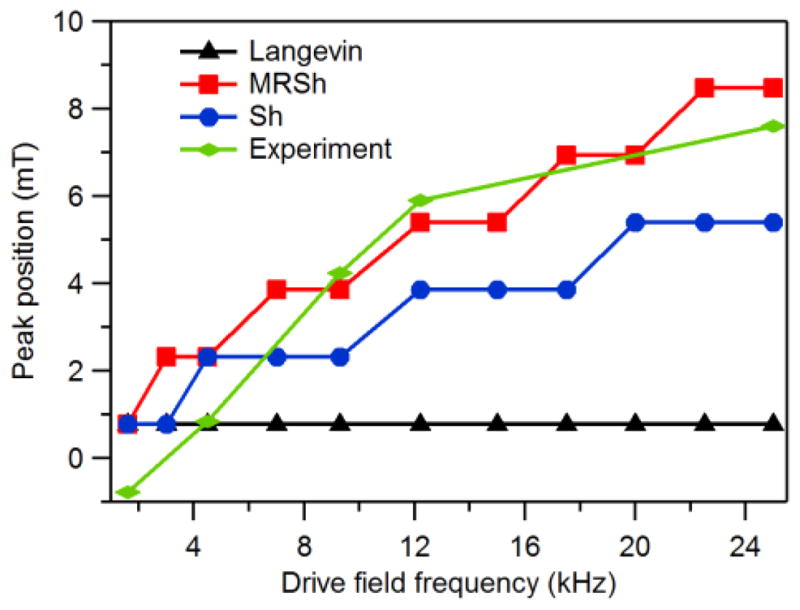
Experimental peak position as a function of drive field frequency is accurately predicted by the MRSh model.
Apart from the peak position, another important piece of information that can be obtained from the PSF is the full width at half maximum (FWHM). The PSF FWHM is one common way to define resolution attainable with a given magnetic nanoparticle for a given field gradient in a MPI scanner. Figure 6 shows the effect of field amplitude on the FWHM for a field frequency of 25 kHz. The experiment predicts the FWHM to decrease at 20 mT and increase thereafter with increasing field amplitude. Interestingly, this feature of the experimental observations was accurately captured by all three models, and thus cannot be used to differentiate among them. The apparent minimum in the FWHM predictions of the Langevin function is attributed to changes in the shape of the signal (illustrated in figures S1 and S2 in the Supplementary Information file) with increasing drive field amplitude at constant frequency. Also, we observed that there is no apparent difference in FWHM between the MRSh and Sh models.
Figure 6.
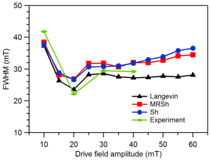
Effect of field amplitude on the full width at half-maximum (FWHM) at a field frequency of 25 kHz.
Finally, to assess the effect of relaxation on the FWHM due to variation in the frequency, we made comparisons between the predictions from models and experiments at constant drive field amplitude of 20 mT, as shown in figure 7. The trend in FWHM for the Langevin function shows slight fluctuations and we believe that they are introduced because of the PSF reconstruction process. Here as well we do not see a significant difference between the predictions of the MRSh and Sh models, with both showing relatively good agreement with the experimentally observed trend. Even though there is a lack of quantitative agreement between the models and experiments on the basis of the FWHM, the agreement between the MRSh model and experiments is quite remarkable in terms of PSF shape and peak position without the need of fitting parameters. According to predictions in our earlier work [22], a significant difference between the MRSh and Sh model would be observed with particles having a core diameter greater than 20 nm. Also, we believe that further improvement in the reconstruction algorithm would improve the FWHM predictions.
Figure 7.
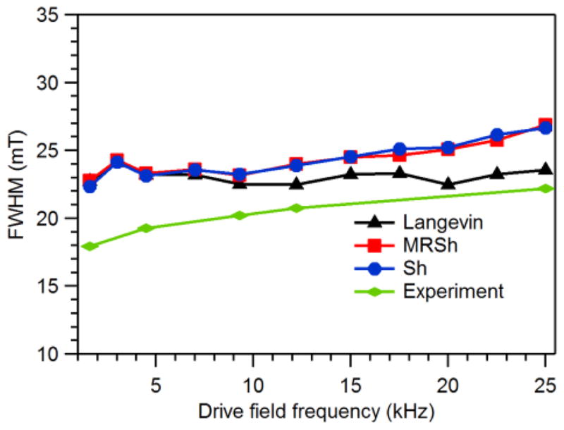
Comparison between the predictions using models and experiments for different field frequencies at an amplitude of 20 mT to assess the effect of relaxation on the FWHM.
5. Conclusions
The experiments and model predictions presented herein demonstrate the potential of the ferrohydrodynamic equations in predicting the performance of magnetic nanoparticles for use in MPI. Particularly, excellent agreement was obtained between the PSFs obtained from predictions of the dynamic magnetization given by the MRSh model and the experimental PSF of magnetic nanoparticles with no fitting parameters used in the model (that is, all magnetic particle properties used in the simulations were independently measured). Of note, only the MRSh model, which incorporates the field-dependence of the magnetic relaxation time, was capable of reproducing the shift in peak position of the PSF, whereas both the MRSh model and the Sh model were able to reproduce the trend in FWHM with changing magnetic field amplitude and frequency. The results presented in this work enable prediction of magnetic nanoparticle behavior in MPI prior to manufacture because the models do not make use of fitting parameters. The models also serve as a platform to better understand the effect of field-dependent relaxation on the performance of particles.
Acknowledgments
This work was supported by the National Institutes of Health (1R21EB018453-01A1). We also gratefully acknowledge funding from the National Science Foundation Graduate Research Fellowship Program, UC Discovery Grant, NIH R01 EB013689, CIRM RT2-01893, Keck Foundation 009323, NIH 1R24 MH106053 and NIH 1R01 EB019458, and ACTG 037829. Steven M. Conolly is a stockholder of Magnetic Insight, Inc, which develops MPI imaging hardware. Patrick W. Goodwill is an employee and stockholder of Magnetic Insight, Inc.
Footnotes
PACS: 47.65.Cb, 41.20.-q, 41.20.Gz
References
- 1.Gleich B, Weizenecker J. Nature. 2005;435:1214–7. doi: 10.1038/nature03808. [DOI] [PubMed] [Google Scholar]
- 2.Weizenecker J, Gleich B, Rahmer J, Dahnke H, Borgert J. Phys Med Biol. 2009;54:L1–L10. doi: 10.1088/0031-9155/54/5/L01. [DOI] [PubMed] [Google Scholar]
- 3.Rahmer J, Antonelli A, Sfara C, Tiemann B, Gleich B, Magnani M, Weizenecker J, Borgert J. Phys Med Biol. 2013;58:3965–77. doi: 10.1088/0031-9155/58/12/3965. [DOI] [PubMed] [Google Scholar]
- 4.Zheng B, von See MP, Yu E, Gunel B, Lu K, Vazin T, Schaffer DV, Goodwill PW, Conolly SM. Theranostics. 2016;6:291–301. doi: 10.7150/thno.13728. [DOI] [PMC free article] [PubMed] [Google Scholar]
- 5.Gleich B, Weizenecker J, Borgert J. Phys Med Biol. 2008;53:N81–4. doi: 10.1088/0031-9155/53/6/N01. [DOI] [PubMed] [Google Scholar]
- 6.Goodwill PW, Conolly SM. IEEE Trans Med Imag. 2010;29:1851–9. doi: 10.1109/TMI.2010.2052284. [DOI] [PubMed] [Google Scholar]
- 7.Goodwill PW, Conolly SM. IEEE Trans Med Imag. 2011;30:1581–90. doi: 10.1109/TMI.2011.2125982. [DOI] [PMC free article] [PubMed] [Google Scholar]
- 8.Croft LR, Goodwill PW, Conolly SM. IEEE Trans Med Imag. 2012;31:2335–42. doi: 10.1109/TMI.2012.2217979. [DOI] [PMC free article] [PubMed] [Google Scholar]
- 9.Goodwill PW, Tamrazian A, Croft LR, Lu CD, Johnson EM, Pidaparthi R, Ferguson RM, Khandhar AP, Krishnan KM, Conolly SM. Appl Phys Lett. 2011;98:262502. [Google Scholar]
- 10.Weizenecker J, Gleich B, Rahmer J, Borgert J. Magnetic nanoparticles : particle science, imaging technology, and clinical applications; proceedings of the First International Workshop on Magnatic Particle Imaging (Institute of Medical Engineering, University of Lübeck, Germany); Singapore ; Hackensack, N.J: World Scientific; 2010. [Google Scholar]
- 11.Goodwill PW, Saritas EU, Croft LR, Kim TN, Krishnan KM, Schaffer DV, Conolly SM. Adv Mater. 2012;24:3870–7. doi: 10.1002/adma.201200221. [DOI] [PubMed] [Google Scholar]
- 12.Weizenecker J, Gleich B, Rahmer J, Borgert J. Phys Med Biol. 2012;57:7317–27. doi: 10.1088/0031-9155/57/22/7317. [DOI] [PubMed] [Google Scholar]
- 13.Reeves DB, Weaver JB. J Appl Phys. 2012;112:124311. doi: 10.1063/1.4770322. [DOI] [PMC free article] [PubMed] [Google Scholar]
- 14.Saritas EU, Goodwill PW, Croft LR, Konkle JJ, Lu K, Zheng B, Conolly SM. J Magn Reson. 2013;229:116–26. doi: 10.1016/j.jmr.2012.11.029. [DOI] [PMC free article] [PubMed] [Google Scholar]
- 15.Ruckert MA, Vogel P, Jakob PM, Behr VC. Biomed Tech. 2013;58:593–600. doi: 10.1515/bmt-2013-0015. [DOI] [PubMed] [Google Scholar]
- 16.Ludwig F, Kuhlmann C, Wawrzik T, Dieckhoff J, Lak A, Kandhar AP, Ferguson RM, Kemp SJ, Krishnan KM. IEEE Trans Magn. 2014;50:5101804. doi: 10.1109/TMAG.2014.2329772. [DOI] [PMC free article] [PubMed] [Google Scholar]
- 17.Enpuku K, Bai S, Hirokawa A, Tanabe K, Sasayama T, Yoshida T. Jpn J Appl Phys. 2014;53:103002. [Google Scholar]
- 18.Bente K, Weber M, Graeser M, Sattel TF, Erbe M, Buzug TM. IEEE Trans Med Imag. 2015;34:644–51. doi: 10.1109/TMI.2014.2364891. [DOI] [PubMed] [Google Scholar]
- 19.Croft LR, Goodwill PW, Konkle JJ, Arami H, Price DA, Li AX, Saritas EU, Conolly SM. Med Phys. 2016;43:424–35. doi: 10.1118/1.4938097. [DOI] [PMC free article] [PubMed] [Google Scholar]
- 20.Dhavalikar R, Rinaldi C. J Appl Phys. 2014;115:074308. [Google Scholar]
- 21.Martsenyuk MA, Raikher YL, Shliomis MI. Sov Phys JETP. 1974;38:413–6. [Google Scholar]
- 22.Dhavalikar R, Maldonado-Camargo L, Garraud N, Rinaldi C. J Appl Phys. 2015;118:173906. doi: 10.1063/1.4935158. [DOI] [PMC free article] [PubMed] [Google Scholar]
- 23.Shliomis MI. Sov Phys JETP. 1972;34:1291–4. [Google Scholar]
- 24.Park J, An KJ, Hwang YS, Park JG, Noh HJ, Kim JY, Park JH, Hwang NM, Hyeon T. Nature Mater. 2004;3:891–5. doi: 10.1038/nmat1251. [DOI] [PubMed] [Google Scholar]
- 25.Rosensweig R. Ferrohydrodynamics. New York: Dover; 1997. [Google Scholar]
- 26.Lu K, Goodwill PW, Saritas EU, Zheng B, Conolly SM. IEEE Trans Med Imag. 2013;32:1565–75. doi: 10.1109/TMI.2013.2257177. [DOI] [PMC free article] [PubMed] [Google Scholar]
- 27.Calero-DdelC VL, Santiago-Quiñonez DI, Rinaldi C. Soft Matter. 2011;7:4497. [Google Scholar]