On the Restricted Mean Survival Time Curve in Survival Analysis

Summary

For a study with an event time as the endpoint, its survival function contains all the information regarding the temporal , stochastic profile of this outcome variable. The survival probability at a specific time point, say t, however, does not transparently capture the temporal profile of this endpoint up to t. An alternative is to use the restricted mean survival time (RMST) at time t to summarize the profile. The RMST is the mean survival time of all subjects in the study population followed up to t, and is simply the area under the survival curve up to t. The advantages of using such a quantification over the survival rate have been discussed in the setting of a fixed-time analysis. In this article, we generalize this approach by considering a curve based on the RMST over time as an alternative summary to the survival function. Inference, for instance, based on simultaneous confidence bands for a single RMST curve and also the difference between two RMST curves are proposed. The latter is informative for evaluating two groups under an equivalence or non-inferiority setting, and quantifies the difference of two groups in a time scale. The proposal is illustrated with the data from two clinical trials, one from oncology and the other from cardiology.

1. Introduction

In a longitudinal study, often the primary endpoint is the time T to a specific event. The corresponding survival function contains all the information about the stochastic features of this endpoint. Empirically this function can be estimated consistently with the Kaplan-Meier (KM) curve with censored event time data (Kaplan and Meier, 1958). When the event rate is low, the empirical cumulative distribution function, which is one minus the KM estimate of the survival function, is generally utilized to display observed event occurrence probabilities over time. The survival/event probability at a specific time point t is a summary measure, which does not contain information regarding the event time distribution profile during the time interval (0, t).

A useful alternative, which summarizes the survival process using information beyond the survival probability only at a single time t, is the restricted mean survival time (RMST) (Irwin, 1949; Zhao and Tsiatis, 1997, 1999; Murray and Tsiatis, 1999; Chen and Tsiatis, 2001; Andersen et al., 2004; Royston and Parmar, 2011; Schaubel and Wei, 2011; Zhao et al., 2012; Tian et al., 2014; Uno et al., 2014). The RMST up to time t is defined as RMST(t) = E(min(T, t)), which is the area under the survival curve of T up to time t. Thus the RMST(t) can be estimated well with the area under the corresponding KM curve up to time t. Note that the area above the survival curve up to time t is the restricted mean time lost, RMTL(t), which is t − RMST(t). With the RMST(t) or RMTL(t) summary measure, one can then construct the corresponding mean survival time curve RMST(·) or RMTL(·) over time, which provides a temporal, stochastic profile of T, expressed in units of time, for evaluating, for example, the benefit or safety of a new therapy. To the best of our knowledge, inference procedures for the RMST curve based on both pointwise and simultaneous confidence intervals and their application have not been discussed in the literature.

For illustration, we use the data from a recent study conducted by the Eastern Cooperative Oncology Group (ECOG) for comparing two groups of patients treated by low- and high-dose dexamethasone for newly diagnosed multiple myeloma (Rajkumar et al., 2010). For this trial, there were 445 enrolled patients: 222 were assigned to the low-dose and 223 to the high-dose group. Figure 1(a) shows the Kaplan-Meier (KM) curves of overall survival based on the data collected by November 2008. The survival curve for the low-dose group (dashed line) is always above the one for the high-dose group (solid line), except at the end of the follow-up. In Figure 1(b), for the KM curve of the low dose group, the area under the curve (darker shaded region) up to t = 40 months is 35.4. That is, on average, the future patients are expected to be alive for 35.4 out of the 40 months of followup. The corresponding estimated RMTL is 40 − 35.4 = 4.6 (months). Figures 1(c) and 1(d) show the corresponding estimated processes RMST(·) and RMTL(·), say, $\widehat{\mathit{RMST}}(\cdot )$ and $\widehat{\mathit{RMTL}}(\cdot )$, respectively, for both the low and high dose groups. This type of the curve provides an interesting alternative to the KM counterpart using a time scale on the y-axis instead of the event or event-free probability. This time scale may be clinically appealing to practitioners with respect to the cost-risk-benefit perspectives for evaluating different treatments. For example, in Figure 1(d), through month 40, the empirical average loss times are 4.6 and 6.7 (months) for the low and high dose groups, respectively, and the difference is 2.1 months with 0.95 confidence interval of (0.1, 4.2) months. That is, with this followup duration, on average, a patient in the high dose group is alive for 2.1 fewer months. On the other hand, the survival rate difference at this time point is -0.04 with a 0.95 confidence interval of (−0.14, 0.06); indicating that there is no significant difference between the two groups. This conclusion, based on survival probabilities, may not reflect the treatment difference appropriately, especially when the study followup time is long and the disease is lethal, such that the two survival curves meet at the end of study.

Figure 1.

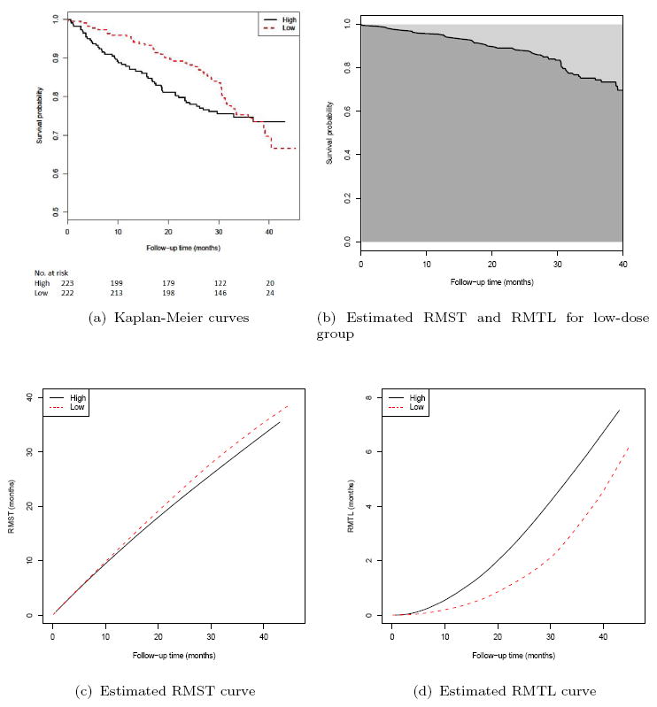
Results based on the data from ECOG (E4A03): (a) Kaplan-Meier curves for high-dose (solid line) and low-dose (dashed line) groups; (b) The estimated RMST (darker shaded region below the solid line) and RMTL (lighter shaded region above the solid line) up to 40 months for the low-dose group; (c) The estimated RMST curve for high-dose (solid line) and low-dose (dashed line) groups; (d) The estimated RMTL curve for high-dose (solid line) and low-dose (dashed line) groups.

In Section 2, we present the inference procedures for the RMST(·) and RMTL(·). Specifically, the pointwise and simultaneous confidence interval estimation procedures for the difference of the two RMSTs over a specific time interval are proposed and illustrated with the data from the above oncology study. This type of analytic tool is quite useful for evaluating the between-group differences under the equivalence/non-inferiority setting. In Section 3, we use the data from a large cardiovascular study to illustrate such an application. Although using a single summary measure for quantifying the group difference is useful for designing the study (for instance, for estimating the study size) and for evaluating the relative merits between treatments under a cost-risk-benefit perspective, a simultaneous inference procedure for the difference of two survival curves or their RMST counterparts can be quite informative. More discussion is provided in the Remarks section.

2. Pointwise and Simultaneous Confidence Interval Estimates

First we consider the case using event time data from a single group, followed by the case for the comparison of two groups. Let T be the time to an event of interest, which may be censored by an independent variable C. For each individual, the observable quantities are (X, Δ), where X = min(T, C) and Δ = I(T ≤ C). The data, {(X_i, Δ_i); i = 1,…, n}, consist of n independent copies of (X, Δ).

Now, let S(t) and Ŝ(t) be the survival function for T and the corresponding KM estimate at time t, respectively. The corresponding RMST(t) and $\widehat{\mathit{RMST}}(t)$ are the areas under S(·) and Ŝ(·) up to t, respectively. It follows from the uniform consistency property of the KM estimator (Gill, 1983) that $\widehat{\mathit{RMST}}(t)$ is uniformly consistent for RMST(t). To derive an approximation to the distribution of $\widehat{\mathit{RMST}}(t)$, we first use the following approximation (Fleming and Harrington, 1991, Page 98):

$$\sqrt{n}\{\widehat{S}(t)-S(t)\}=-\sqrt{n}S(t)\sum _{i=1}^n{\int }_0^t\frac{d{M}_i(u)}{\overline{Y}(u)}+o_p(\mathrm{l}),$$

where $M_i(t)=N_i(t)-{\int }_0^t{Y}_i(u)\lambda (u)\mathit{du}$, $N_i(t)=I\{X_i\le t,{\mathrm{\Delta }}_i=1\}$, $Y_i(t)=I\{X_i\ge t\}$, $\overline{Y}(t)={\sum }_{i=1}^n{Y}_i(t)$ and λ(t) is the hazard function for T. Note that due to right censoring, this approximation is only valid for the interval t ∊ [0, τ], where pr(X > τ) > 0. It follows from the martingale central limit theorem (Fleming and Harrington, 1991, Chapter 5) that $\sqrt{n}\{\widehat{S}(t)-S(t)\}$ converges weakly to a Gaussian process over the interval [0, τ].

With the functional δ-method, the distribution of $\sqrt{n}\left\{\widehat{\mathit{RMST}}(\cdot )-\mathit{RMST}(\cdot )\right\}$ can be approximated asymptotically by that of a mean-zero Gaussian process G(·). When the sample size is large, this limiting distribution can be approximated well via a perturbation-resampling method (Lin et al., 1993; Parzen et al., 1997; Zhao et al., 2012). Specifically, let {Z_i, i = 1, ….n} be n random samples from N(0, 1), which are independent of the data. Then the distribution of $\sqrt{n}\{\widehat{S}(t)-S(t)\}$ can be approximated by the distribution (conditional on the data) of

$$L^{\ast }(t)=\sqrt{n}\widehat{\mathbb{S}}(t)\sum _{i=1}^n{Z}_i{\int }_0^t\frac{d{\mathbb{N}}_i(u)}{\mathbb{Y}(u)},$$

where Ŝ(·), Ȳ(·) and ℕ_i(·) denote the observed quantities from the data for Ŝ(·), Ȳ(·) and N_i(·), respectively. That is, the distribution of $\sqrt{n}\{\widehat{S}(t)-S(t)\}$ can be approximated using a large number of sets for the perturbation weights {Z_i, i =1, ⋯, n} given the observed data. This technique has been successfully utilized in many applications in survival analysis (Park and Wei, 2003; Tian et al., 2005; Cai et al., 2010).

Now, to approximate G(·), the limiting Gaussian process, one can simply consider the random process over t ∊ [0, τ]:

$${\int }_0^t{L}^{\ast }(s)\mathit{ds}.$$ (1)

Note that the conditional asymptotic distribution of (1) is G(·). Such a conditional distribution can be approximated by its empirical counterpart based on realizations from M different sets of random perturbation weights {Z_i : i = 1, …, n} Let the corresponding standard deviation estimate for the distribution of G(·) be denoted by σ̂_R(·). The pointwise confidence interval estimate for the RMST(·) can be constructed based on the standard normal approximation to $\sqrt{n}\left(\widehat{\mathit{RMST}}(t)-\mathit{RMST}(t)\right)/{\widehat{\sigma }}_R(t)$. Specifically, for any α ∊ (0, 1), a two-sided 1 − α confidence interval for RMST(t) is

$$\left(\widehat{\mathit{RMST}}(t)-z_{(1-\alpha /2)}{n}^{-1/2}{\widehat{\sigma }}_R(t),\widehat{\mathit{RMST}}(t)+z_{(1-\alpha /2)}{n}^{-1/2}{\widehat{\sigma }}_R(t)\right),$$

where z_(1−α/2) is the 100(1−α/2)-th percentile of the standard normal distribution. Note that in theory, the above confidence interval estimation procedure is valid for t ∊ [η, τ], where pr(T < η) > 0 and pr(X > τ) > 0. The corresponding simultaneous, equal precision confidence interval (Nair, 1984) estimate for RMST(t) over [η, τ] would be

$$\left(\widehat{\mathit{RMST}}(t)-c_{\alpha }{n}^{-1/2}{\widehat{\sigma }}_R(t),\widehat{\mathit{RMST}}(t)+c_{\alpha }{n}^{-1/2}{\widehat{\sigma }}_R(t)\right),$$

where the cutoff value c_α is chosen such that

$$\mathrm{p}\mathrm{r}\left(\underset{t\in [\eta ,\tau ]}{\sup }\mid \frac{{\int }_0^t{L}^{\ast }(s)\mathit{ds}}{{\widehat{\sigma }}_R(t)}\mid \le c_{\alpha }\right)\ge 1-\alpha .$$

In practice, the time interval [η, τ] can be chosen by requiring that the estimated probabilities for both pr(T < η) and pr(X > τ), which can be obtained from the KM estimates for the distributions of T and the empirical cumulative distribution function of X, respectively, are greater than a small positive number d. This truncation is to ensure the positivity of σ̂_R(t) and the statistical validity of the interval estimation procedure. Note that this requirement is satisfied as long as η is greater than the smallest observed event time and τ is less than the maximum follow up time (Gill, 1983). The pointwise and simultaneous confidence intervals for RMTL(t) can be similarly constructed using the fact that RMTL(t) = t − RMST(t).

As an example, with the data from the low dose group from the cancer study and with M = 1000 realizations of {Z_i : i = 1,…, n} from the standard normal distribution, the 0.95 pointwise (dashed lines) and simultaneous (shaded area) confidence intervals for the RMTL(·) are given in Figure 2(a). Here, the time interval for the simultaneous confidence intervals is [η, τ] = [0.2, 40] months, where the choice of η = 0.2 is the smallest time satisfying the condition that the estimated probability of pr(T < η) is positive, and the choice of η = 40 satisfies the condition that the estimated probability of pr(X < τ) is positive and was considered by Uno et al. (2014). These confidence bands are quite informative. For instance, at Month 40, the possible values for RMTL are between 3.1 months and 6.1 months based on the 0.95 simultaneous confidence band. Note that the simultaneous confidence band quantifies the uncertainty in estimating the entire RMST curve over [0.2, 40]. Thus no single time point t needs to be pre-specified.

Figure 2.

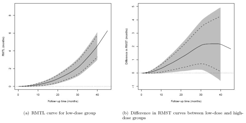
Results based on the data from ECOG (E4A03): (a) RMTL curve for lowdose group; (b) Difference in RMST curves between low-dose and high-dose groups. Solid lines: point estimates, dashed lines: pointwise 0.95 confidence intervals, shaded region: simultaneous 0.95 confidence intervals, dotted line: zero reference line.

Now, suppose that we are interested in estimating the difference of two RMST curves. Let all the aforementioned random variables and observed quantities be indexed by k = 1, 2 for the two treatment groups. The data are {(X_1i, Δ_1i); i = 1, …, n₁} for group 1 and {(X_2j, Δ_2j); j = 1, …, n₂} for group 2. Let D(t) = RMST₂(t) − RMST₁(t). Then, it follows that $\widehat{D}(t)={\widehat{\mathit{RMST}}}_2(t)-{\widehat{\mathit{RMST}}}_1(t)$ is uniformly consistent for D(t), for t ∊ [0, τ], where pr(X₁₁ > τ)pr(X₂₁ > τ) > 0. Moreover, n^−1/2(D̂(·) − D(·)) converges weakly to the Gaussian G₂(·) − G₁(·), whose distribution can be approximated by the realizations of the differences of the two corresponding process (1) for the two treatment groups.

Let the standard deviation estimate for G₂(·)−G₁(·) be denoted by σ̂_D(t) via the perturbation method with M independent sets of random weights {Z_1i, i = 1, …, n₁; Z_2j, j = 1, ⋯, n₂}. Then the pointwise confidence interval estimate for D(t) is

$$\left(\widehat{D}(t)-z_{(1-\alpha /2)}{n}^{-1/2}{\widehat{\sigma }}_D(t),\widehat{D}(t)+z_{(1-\alpha /2)}{n}^{-1/2}{\widehat{\sigma }}_D(t)\right),$$

and the corresponding simultaneous, equal precision confidence interval estimate over the range [η, τ] is

$$\left(\widehat{D}(t)-{\stackrel{\sim }{c}}_{\alpha }{n}^{-1/2}{\widehat{\sigma }}_D(t),\widehat{D}(t)+{\stackrel{\sim }{c}}_{\alpha }{n}^{-1/2}{\widehat{\sigma }}_D(t)\right),t\in [\eta ,\tau ],$$

where pr(T₁₁ < η)pr(T₂₁ < η) > 0, and the cutoff point c̃_α satisfies that

$$\mathrm{Pr}\left(\underset{t\in [\eta ,\tau ]}{\sup }\mid \frac{{\int }_0^t\left[L_2^{\ast }(s)-L_1^{\ast }(s)\right]\mathit{ds}}{{\widehat{\sigma }}_D(t)}\mid \le {\stackrel{\sim }{c}}_{\alpha }\right)\ge 1-\alpha .$$

Empirically, [η, τ] can be chosen such that the estimated probabilities of both pr(T₁₁ < η)pr(T₂₁ < η) and pr(X₁₁ > τ)pr(X₂₁ > τ) are greater than a small positive number d.

As an example, with the data from the cancer study, Figure 2(b) shows the 0.95 pointwise and simultaneous confidence interval estimates for D(t). Here, the time interval for simultaneous confidence intervals is [η, τ] = [0.7, 40] months, where the choice of η = 0.7 is the smallest time satisfying the condition that the estimated probability of pr(T₁₁ < η)pr(T₂₁ < η) is positive. Note that for this study, the hazard ratio estimate is 0.87 in favor of the low dose, but with a 0.95 confidence interval of (0.60, 1.27) that does not detect a significant difference between groups, possibly due to the fact that the two hazard functions are crossed. On the other hand, except for the small time interval near 40 months, the lower bounds of the 0.95 simultaneous confidence intervals are above the null value of zero, indicating that the patients in the low dose group tend to live longer than those in the high dose group. For example, at month 20, the difference in RMST is 1.1 months with a 0.95 pointwise confidence interval of (0.4, 2.0) and the corresponding simultaneous confidence interval of (0.1, 2.2) months. Note that in this example the low dose group is still significantly better than the high dose group in RMST at month 20, after adjusting for the multiple comparisons over the entire time interval [0.7, 40] months using the simultaneous confidence band.

As suggested by a referee, it is interesting to note that using the simultaneous confidence band for the difference of two survival curves may give us different perceptions of the relative merits of the two dose groups. Figure 3 shows the 0.95 pointwise amd simultaneous confidence intervals for the difference of two survival curves with the data from the above cancer study. For this case, the lower bounds of the pointwise confidence interval are well below the null value of zero beyond 30 months, and the lower bounds of the simultaneous confidence interval are below the null value of zero for almost the entire time interval of [0.7, 40] months.

Figure 3.

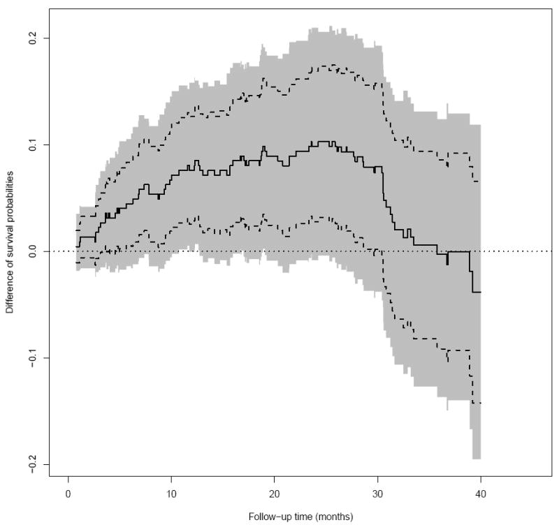
The difference in survival probability at different time points between lowdose and high-dose groups of patients in the ECOG (E4A03) study (Solid: point estimate; Dashed: 0.95 pointwise confidence interval; Shaded: 0.95 simultaneous confidence interval; dotted: zero reference line).

We also present a hazard ratio plot in Figure 4, where at each time point t, the hazard ratio estimate (y-axis) is obtained via all the survival data censored at time t. The hazard ratio estimate is unstable for small t due to too few events. Here, we chose a narrower time interval of [4.5, 40] to explore the profile of the confidence band. Note that the 0.95 simultaneous confidence band is quite wide and contains the null value of zero for almost the entire time interval of [4.5, 40] months.

Figure 4.

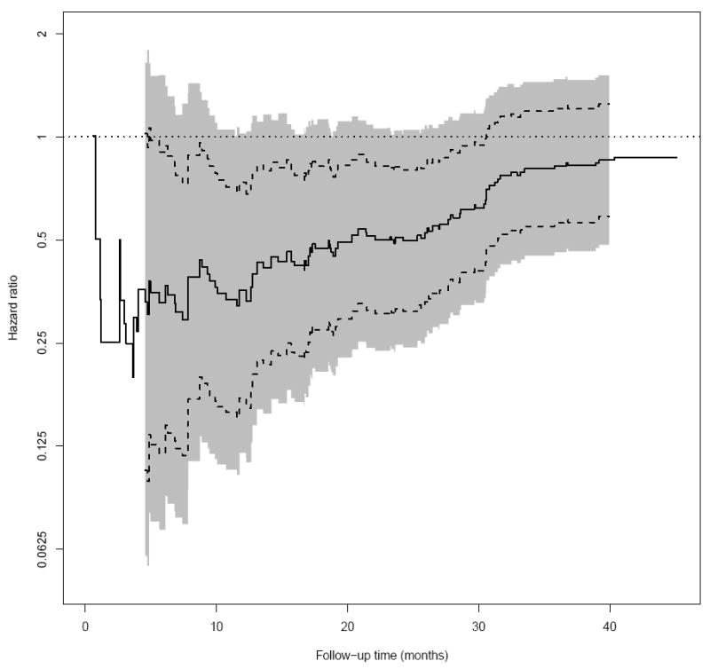
The hazard ratio for different censoring cutoff time points between low-dose and high-dose groups of patients in the ECOG (E4A03) study (Solid: point estimate; Dashed: 0.95 pointwise confidence interval; Shaded: 0.95 simultaneous confidence interval; dotted: one reference line).

In this example, while the survival time in low dose group is stochastically greater than that in the high dose group, the difference in survival probability at a single point or hazard ratio may fail to reflect this difference due to the crossing hazard functions. The RMST appears to be a more appropriate summary in this setting. On the other hand, any single summary measure, including RMST at a fixed time point, still may fail to provide an adequate summary of the treatment effect under a particular alternative hypothesis and we recommend to examine the RMST process over the entire time span of interest.

3. An application of the simultaneous confidence band estimation procedure for comparative studies under an equivalence/non-inferiority setting

In this section, we use the data from a cardiovascular trial: “Valsartan In Acute Myocardial Infarction (VALIANT) Study” (Pfeffer et al., 2003) to illustrate our inference proposal for evaluating equivalence of two treatment groups with respect to the patient’s survival. There were three arms for the study, the patients in the first group were treated by valsartan, the second group was with captopril and the third one was with a combination of these two drugs. One of the study goals was to investigate if the two mono-therapies were equivalent with respect to the overall survival. The study was conducted from 1999 to 2003 with a total of 9818 patients equally assigned to the above two mono-therapy groups. The median follow-up time is 24.7 months after randomization. Figure 5 shows the KM curves for two arms with mono-therapies, which visually are overlapped with each other over 46 months of follow-up. The hazard ratio estimate is 1.02 with a 0.95 confidence interval of (0.93, 1.11). Using the technique discussed in Section 2, the 0.95 pointwise and simultaneous confidence intervals for two RMST functions are given in Figure 6. Note that the confidence bands are constructed using M = 1000 realizations of the standard normal random sample for the resampling method and [η, τ] = [0.1, 45.5] months, which is the maximum-length time interval such that the estimated probabilities for both pr(T₁₁ < η)pr(T₂₁ < η) and pr(X₁₁ > τ)pr(X₂₁ > τ) are positive empirically. With this simultaneous confidence band, one can assess an equivalence or non-inferiority claim for two treatment groups over the entire study time period of interest, not only via the treatment difference at a single specific time point or a single summary measure of the treatment difference curve. This quantitative procedure provides an alternative way for an equivalence/non-inferiority evaluation. For instance, at 10, 20, 30 and 40 months, with 0.95 confidence level, the true RMST differences between the two groups would be simultaneously in a rectangular region of (−0.1, 0.2)×(−0.2, 0.4)×(−0.4, 0.6)×(−0.7, 0.7) in the unit of months. The tight confidence band in Figure 6 suggests that there is no clinically meaningful difference between two mono-therapies with respect to the patient’s survival over the entire study time period of interest.

Figure 5.

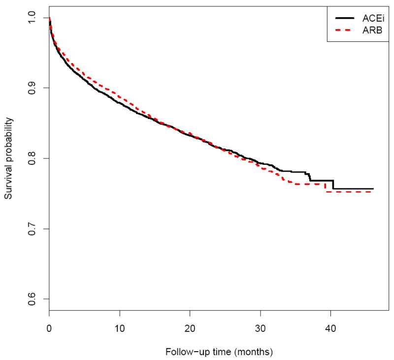
The Kaplan-Meier estimates for the survival functions of patients taking ARB or ACEi in the VALIANT study.

Figure 6.

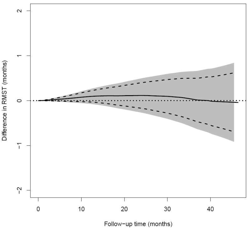
The difference in RMST curves between ARB and ACEi in RMST up to time t of patients in the VALIANT study (Solid: point estimate; Dashed: 0.95 pointwise confidence interval; Shaded: 0.95 simultaneous confidence interval; dotted: zero reference line).

4. Remarks

The survival curve estimate in Figure 1(a) contains all the information empirically regarding the temporal profile of the survivorship of patients in each dose group for the ECOG study. On the other hand, the corresponding RMTL curve estimates presented in 1(c) may provide a different perspective to visually characterizing the difference in survival distributions. For instance, the observed survival probability for the low dose group at month 40 is numerically smaller than that for the high dose group (0.70 vs. 0.74). However, this could also be equally true under a scenario where 30% of low-dose patients died on day 1 of the study as well as the scenario where all low-dose patients survive until month 39. These two scenarios can be distinguished by either examining the entire survival curves or RMST evaluated at month 40. Note that the RMST curve for the low dose group is above that of the high dose group almost over the entire 40 month follow-up. Both types of curve estimates can be useful, depending on the clinical question of interest, and may complement each other to describe and interpret the survivorship patterns associated with the intervention(s) of interest.

The choice of the time interval [η, τ] is crucial since the resulting confidence bands for the difference of RMST curves depend on the choice of this time interval. This issue also applies to the case for the simultaneous inference about the difference of two survival curves or hazard ratio. Empirically one may choose the largest possible time interval for which a valid inference claim for the difference of two curses can be made as discussed in Section 3. If a time interval is pre-specified in the study protocol based on the clinical interest, the final choice of the interval may be the intersection of these two intervals.

For the purpose of evaluating whether two regimens are equivalent with respect to an event time outcome, the conventional approach is to utilize an event-driven study and summarize the comparison via, for example, an estimated confidence interval for the hazard ratio. This approach is not ideal and may be misleading. For example, for the cancer study example, a 0.95 confidence interval for the hazard ratio between two dose groups is (0.60, 1.27), which includes the null value one. One may interpret this result to indicate that there is not enough information to make a decision or that there is no difference statistically. The concerns and issues regarding the use of the hazard ratio as a between-group difference measure in survival analysis in the superiority and non-inferiority study settings have been discussed (Uno et al., 2014, 2015). The simultaneous confidence band for the difference of two RMST (RMTL) curves presented in this article, expressed in units of time, would be a useful addition to address the equivalence or non-inferiority question via a time scale.

References

- Andersen PK, Hansen MG, Klein JP. Regression analysis of restricted mean survival time based on pseudo-observations. Lifetime Data Analysis. 2004;10:335–350. doi: 10.1007/s10985-004-4771-0. [DOI] [PubMed] [Google Scholar]
- Cai T, Tian L, Uno H, Solomon SD, Wei LJ. Calibrating parametric subject-specific risk estimation. Biometrika. 2010;97:389–404. doi: 10.1093/biomet/asq012. [DOI] [PMC free article] [PubMed] [Google Scholar]
- Chen PY, Tsiatis AA. Causal inference on the difference of the restricted mean lifetime between two groups. Biometrics. 2001;57:1030–1038. doi: 10.1111/j.0006-341x.2001.01030.x. [DOI] [PubMed] [Google Scholar]
- Fleming TR, Harrington DP. Counting processes and survival analysis. Vol. 8. Wiley Online Library; 1991. [Google Scholar]
- Gill R. Large sample behaviour of the product-limit estimator on the whole line. The Annals of Statistics. 1983;11:49–58. [Google Scholar]
- Irwin JO. The standard error of an estimate of expectation of life, with special reference to expectation of tumourless life in experiments with mice. Journal of Hygiene. 1949;47:188–189. doi: 10.1017/s0022172400014443. [DOI] [PMC free article] [PubMed] [Google Scholar]
- Kaplan EL, Meier P. Nonparametric estimation from incomplete observations. Journal of the American statistical association. 1958;53:457–481. [Google Scholar]
- Lin DY, Wei LJ, Ying Z. Checking the cox model with cumulative sums of martingale-based residuals. Biometrika. 1993;80:557–572. [Google Scholar]
- Murray S, Tsiatis AA. Sequential methods for comparing years of life saved in the two-sample censored data. Biometrics. 1999;55:1085–1092. doi: 10.1111/j.0006-341x.1999.01085.x. [DOI] [PubMed] [Google Scholar]
- Nair VN. Confidence bands for survival functions with censored data: a comparative study. Technometrics. 1984;26:265–275. [Google Scholar]
- Park Y, Wei LJ. Estimating subject-specific survival functions under the accelerated failure time model. Biometrika. 2003;90:717–723. [Google Scholar]
- Parzen MI, Wei LJ, Ying Z. Simultaneous confidence intervals for the difference of two survival functions. Scandinavian Journal of Statistics. 1997;24:309–314. [Google Scholar]
- Pfeffer MA, McMurray JJV, Velazquez EJ, Rouleau J-L, Køber L, Maggioni AP, Solomon SD, Swedberg K, Van de Werf F, White H, Leimberger JD, Henis M, Edwards S, Zelenkofske S, Ann Sellers M, Califf RM. Valsartan, captopril, or both in myocardial infarction complicated by heart failure, left ventricular dysfunction, or both. New England Journal of Medicine. 2003;349:1893–1906. doi: 10.1056/NEJMoa032292. [DOI] [PubMed] [Google Scholar]
- Rajkumar SV, Jacobus S, Callander NS, Fonseca R, Vesole DH, Williams ME, Abonour R, Siegel DS, Katz M, Greipp PR. Lenalidomide plus high-dose dexamethasone versus lenalidomide plus low-dose dexamethasone as initial therapy for newly diagnosed multiple myeloma: an open-label randomised controlled trial. The lancet oncology. 2010;11:29–37. doi: 10.1016/S1470-2045(09)70284-0. [DOI] [PMC free article] [PubMed] [Google Scholar]
- Royston P, Parmar MKB. The use of restricted mean survival time to estimate the treatment effect in randomized clinical trials when the proportional hazards assumption is in doubt. Statistics in medicine. 2011;30:2409–2421. doi: 10.1002/sim.4274. [DOI] [PubMed] [Google Scholar]
- Schaubel DE, Wei G. Double inverse-weighted estimation of cumulative treatment effects under nonproportional hazards and dependent censoring. Biometrics. 2011;67:29–38. doi: 10.1111/j.1541-0420.2010.01449.x. [DOI] [PMC free article] [PubMed] [Google Scholar]
- Tian L, Zhao L, Wei LJ. Predicting the restricted mean event time with the subject’s baseline covariates in survival analysis. Biostatistics. 2014;15:222–233. doi: 10.1093/biostatistics/kxt050. [DOI] [PMC free article] [PubMed] [Google Scholar]
- Tian L, Zucker D, Wei LJ. On the cox model with time-varying regression coefficients. Journal of the American statistical Association. 2005;100:172–183. [Google Scholar]
- Uno H, Claggett B, Tian L, Inoue E, Gallo P, Miyata T, Schrag D, Takeuchi M, Uyama Y, Zhao L, Skali H, Solomon S, Jacobus S, Hughes M, Packer M, Wei LJ. Moving beyond the hazard ratio in quantifying the between-group difference in survival analysis. Journal of Clinical Oncology. 2014;32:2380–2385. doi: 10.1200/JCO.2014.55.2208. [DOI] [PMC free article] [PubMed] [Google Scholar]
- Uno H, Wittes J, Fu H, Solomon SD, Claggett B, Tian L, Cai T, Pfeffer MA, Evans SR, Wei LJ. Alternatives to hazard ratios for comparing the efficacy or safety of therapies in noninferiority studies. Annals of Internal Medicine. 2015 doi: 10.7326/M14-1741. To appear. [DOI] [PMC free article] [PubMed] [Google Scholar]
- Zhao H, Tsiatis AA. A consistent estimator for the distribution of quality adjusted survival time. Biometrika. 1997;84:339–348. [Google Scholar]
- Zhao H, Tsiatis AA. Efficient estimation of the distribution of quality-adjusted survival time. Biometrics. 1999;55:1101–1107. doi: 10.1111/j.0006-341x.1999.01101.x. [DOI] [PubMed] [Google Scholar]
- Zhao L, Tian L, Uno H, Solomon SD, Pfeffer MA, Schindler JS, Wei LJ. Utilizing the integrated difference of two survival functions to quantify the treatment contrast for designing, monitoring, and analyzing a comparative clinical study. Clinical Trials. 2012;9:570–577. doi: 10.1177/1740774512455464. [DOI] [PMC free article] [PubMed] [Google Scholar]
Associated Data
This section collects any data citations, data availability statements, or supplementary materials included in this article.