A Charge Central Interpretation of the Full Nonlinear PB Equation: Implications to Accurate and Scalable Modeling of Solvation Interactions

Abstract

Continuum solvation modeling based upon the Poisson-Boltzmann equation (PBE) is widely used in structural and functional analysis of biomolecules. In this work we proposed a charge-central interpretation of the full nonlinear PBE electrostatic interactions. The validity of the charge-central framework, as formulated as a vacuum Poisson equation with effective charges, was first demonstrated by reproducing both electrostatic potentials and energies from the original solvated full nonlinear PBE. There are at least two benefits when the charge-central framework is applied. Firstly the convergence analyses show that the use of polarization charges allows a much faster converging numerical procedure for electrostatic energy and forces calculation for the full nonlinear PBE. Secondly the formulation of the solvated electrostatic interactions as effective charges in vacuum allows scalable algorithms to be deployed for large biomolecular systems. Here we exploited the charge-central interpretation and developed a particle-particle particle-mesh (P3M) strategy for the full nonlinear PB systems. We also studied the accuracy and convergence of solvation forces with the charge-view and the P3M methods. It is interesting to note that the convergences of both the charge-view and the P3M methods are more rapid than the original full nonlinear PB method. Given the developments and validations documented here, we are working to adapt the P3M treatment of the full nonlinear PB model to molecular dynamics simulations.

Graphical Abstract

Introduction

Life as we know it occurs in water so that inclusion of water is crucial to model the structures and functions of biomolecules accurately.^1–19 Since the cost of explicitly including water molecules in computer models is very high, approximating water interactions implicitly or in a continuum manner is a widely used strategy in computational studies of biomolecules.^1–18 A key component in such approaches is the electrostatic solvation modeling based on the Poisson-Boltzmann equation (PBE). A number of pioneer works have been published to study the solvation electrostatic effects in biomolecular functions.^{1–18, 20} In these studies, numerical solution of the PBE is crucial because of the irregular shapes of biomolecules.^{3, 21–26} Currently, the finite-difference method,^27–42 finite-element method^43–51 and boundary-element method^52–68 are the most widely used numerical methods.

Due to its numerical nature, there are difficulties to incorporate PBE methods into molecular mechanics simulations, such as interpolating electrostatic forces, removing singular atomic charges,^{35, 43, 69–79} and achieving faster numerical convergence.^80–82 Currently the numerical PBE methods are only applied in situations where a few fixed conformations are involved, limiting the potentials of the methods. Efforts have been invested to improve these numerical issues of the PBE methods^{35, 43, 57, 69–79, 83–90} in order to facilitate the incorporation of the model in molecular mechanics simulations. The “virtual work” method, which computes forces according to the numerical derivative of potential energy, is apparently the benchmark for all analytical methods, but it is only realistic when molecules are treated as rigid bodies. Thus analytical calculation of solvation forces is necessary for in most situations. Two broadly different schemes have been developed to interpolate solvation forces. For the classical abrupt-transitioned two-dielectric models, multiple strategies have been proposed by Davis and McCammon,⁶⁹ Che et al.,⁷⁴ Bo et al.,⁷⁶ Cai et al.⁷⁷ and most recently Li et al.⁷⁹. These formulations were derived following different strategies and were found to be consistent. For the smooth-transitioned dielectric models, we have the ground-breaking strategy by Gilson et al..⁷³ Subsequent works by Im et al.³⁵ and Cai et al.⁷⁵ were shown to be consistent with that of Gilson et al.,⁷³ though different strategies were proposed to enhance numerical stability and convergence in the later works. The numerical methods derived from these formulations are mostly adapted for the numerical solutions by the finite-difference method. Boundary-element method is another promising approach to incorporate the PBE electrostatics into molecular mechanics simulations. The force calculation in a boundary-element calculation was first described by Zauhar.⁷¹ In addition, Cortis et al.⁴³ explored to compute the solvation force for their finite-element method calculations, leading to the same formulation as that of Zauhar.⁷¹

In this study we address this issue in the context of full nonlinear PBE, which is useful in modeling of highly charged systems, i.e. nucleic acids or nucleic acid-binding proteins or ligands. Specifically we explored a charge central interpretation of the full PBE potentials and energies, which is to use the effective charge density to compute all electrostatic potentials, energies, and forces. There are at least two benefits in developing this strategy. Firstly the use of polarization charges allows a much faster converging numerical procedure for electrostatic energy and forces calculation for the Poisson’s equation and linear PBE as we have shown,^{75, 77, 82} and also for the full nonlinear PBE as shown below. Secondly the formulation of the solvated electrostatic interactions as effective charges in vacuum allows scalable algorithms to be deployed for large biomolecular systems. For example, we have explored to adapt the particle-particle particle-mesh (P3M) strategy for fully solvated electrostatic interactions as modeled by the full nonlinear PBE. P3M is a typical method for accurate and efficient calculation of Coulombic interactions of biomolecular systems.^91–93 Apparently P3M cannot be used directly in calculating energy and forces based on the nonlinear PBE because there are heterogeneous dielectrics in the solute and solvent regions. In the following we first present the charge-central strategy to model the full nonlinear PBE potentials, energies, and forces. This is followed by numerical implementations and how to use P3M to balance accuracy and efficiency in applying nonlinear PBE to complex molecular systems.

Theory and Computational Details

A. Effective charge interpretation of Poisson-Boltzmann equation

The full nonlinear PBE for systems with continuum mobile ions can be expressed as

$$\nabla •(\epsilon \nabla \varphi )=-4\pi {\rho }^f-4\pi \sum _i{e}_i{c}_{i}exp\left(-e_i\varphi /k_{B}T\right)\lambda$$ (1)

Where ϕ is the potential, ε is the dielectric constant, e_i is the charge of ion type i, c_i is the bulk number density of ion type i, λ is the ion exclusion function, k_B is the Boltzmann constant and T is the absolute temperature. Following our developments for the Poisson equation^{75, 77, 82}, the solution of the PBE can be cast into a vacuum Poisson equation with effective charges only, as shown in detail in Appendix A. Briefly, consider a solute molecule with dielectric constant ε_i surrounded by a solvent medium with dielectric constant ε_o, the solution of the original PBE satisfies a vacuum Poisson equation in the form of

$${\nabla }^2\varphi =-4\pi \left(\frac{{\rho }^f}{{\epsilon }_i}+\frac{{\rho }^m}{{\epsilon }_o}+{\rho }^{\mathit{pol}}\right),$$ (2)

where

$$\begin{array}{l}\varphi ={\varphi }_C^f+{\varphi }_C^m+{\varphi }_{RF}\hfill \\ {\epsilon }_i{\nabla }^2{\varphi }_C^f=-4\pi {\rho }^f\hfill \\ {\epsilon }_o{\nabla }^2{\varphi }_C^m=-4\pi {\rho }^m\hfill \\ {\nabla }^2{\varphi }_{RF}=-4\pi {\rho }^{\mathit{pol}}\hfill \\ {\rho }^m=\sum _i{e}_i{c}_{i}exp\left(-e_i\varphi /k_{B}T\right)\lambda \hfill \end{array}.$$ (3)

Here ϕ_C is the Coulomb potential generated by solute charges (denoted by superscript f) or mobile ion charges (denoted by superscript m) in their respective uniform dielectric media throughout the whole space and ϕ_RF is the total reaction field potential.

It is worth pointing out that the equivalence of eqn (2) to eqn (1) is not based on the superposition principle, which does not hold for nonlinear partial differential equations in general. In addition the effective source terms ρ^m and ρ^pol cannot be known before solving eqn (1) via standard numerical procedures. A more rigorous presentation is also possible via the integral form utilizing the Green’s theorem.⁹⁴ However, it is more physically intuitive by following the discussion presented here.

There are at least two benefits when the charge-central framework is applied. Firstly the use of polarization charges allows a much faster converging numerical procedure for electrostatic energy and forces calculation for the full nonlinear PBE as shown below. Secondly many efficient numerical algorithms developed to speed up vacuum electrostatic/Coulombic field calculation can now be applied to the full PBE systems if the effective charge sources can be obtained, which will be discussed below.

B. Total electrostatic energy and forces of Poisson-Boltzmann systems

The total electrostatic energy of a Poisson-Boltzmann system can be written as⁸⁷

$$\begin{array}{l}G=\int \left({\rho }^f\varphi -\frac{1}{8\pi }\mathbf{D}•\mathbf{E}-\mathrm{\Delta }\mathrm{\Pi }\lambda \right)dv\\ \mathrm{\Delta }\mathrm{\Pi }=kT\sum _l{c}_l(e^{-q_l\varphi /kT}-1)\end{array}$$ (4)

Substitution of the PBE into eqn (4) leads to

$$G=\int \left(\frac{{\rho }^f\varphi }{2}-\frac{{\rho }^m\varphi }{2}-\mathrm{\Delta }\mathrm{\Pi }\lambda \right)dv.$$ (5)

Eqn (5) suggests that G be decomposed into three parts as G = G^f + G^m + G^Π. Here G^Π is the entropic term due to the excess osmotic pressure, apparently not due to charge-charge interactions so that no further treatment is attempted below. In contrast, G^f and G^m can be reformulated according to the effective charge view presented above.

Substitution of $\varphi ={\varphi }_C^f+{\varphi }_C^m+{\varphi }_{RF}$ into the first term of eqn (5) leads to

$$G^f=\frac{1}{2}\int {\rho }^f({\varphi }_C^f+{\varphi }_C^m+{\varphi }_{RF})dv$$ (6)

Apparently G^f can be decomposed into three parts:

$$\begin{array}{l}{G}^f=G_C^f+G_m^f+G_{\mathit{pol}}^f\\ G_C^f=\frac{1}{2}\int {\rho }^f{\varphi }_C^{f}dv\\ G_m^f=\frac{1}{2}\int {\rho }^f{\varphi }_C^{m}dv\\ G_{\mathit{pol}}^f=\frac{1}{2}\int {\rho }^f{\varphi }_{RF}dv\end{array}$$ (7)

Thus the electrostatic energy associated with the fixed charges on the atoms is due to interactions with other atomic charges, mobile ion charges, and overall induced polarization charges.

Similarly the second term of eqn (5) can be written as follows upon the substitution of $\varphi ={\varphi }_C^f+{\varphi }_C^m+{\varphi }_{RF}$

$$\begin{array}{ll}{G}^m\hfill & =G_C^m+G_m^m+G_{\mathit{pol}}^m\hfill \\ G_C^m\hfill & =-\frac{1}{2}\int {\rho }^m{\varphi }_C^{f}dv=-\frac{{\epsilon }_o}{2{\epsilon }_i}\int {\rho }^f{\varphi }_C^{m}dv\hfill \\ G_m^m\hfill & =-\frac{1}{2}\int {\rho }^m{\varphi }_C^{m}dv\hfill \\ G_{\mathit{pol}}^m\hfill & =-\frac{1}{2}\int {\rho }^m{\varphi }_{RF}dv\hfill \end{array}$$ (8)

Thus the electrostatic energy associated with the mobile ion charges is due to interactions with atomic charges, other mobile ion charges, and overall induced polarization charges. Overall the conclusions in eqn (7) and (8) are consistent with the Coulomb’s law once the effective charge view of the PBE system is used.

We now turn to the formulation of electrostatic forces. Given the discussion in Refs ^{75, 77}, the force density is the divergence of the Maxwell stress tensor⁹⁵ for systems without singularities or discontinuities

$$\begin{array}{l}\nabla •\mathbf{P}=\frac{\partial }{\partial x}(\mathit{i}•\mathbf{P})+\frac{\partial }{\partial y}(\mathit{j}•\mathbf{P})+\frac{\partial }{\partial z}(\mathit{k}•\mathbf{P})\\ ={\rho }^f\mathbf{E}-\frac{1}{8\pi }{\mathbf{E}}^2\nabla \epsilon -\mathrm{\Delta }\mathrm{\Pi }\nabla \lambda \end{array}$$ (9)

which is consistent with the formulation derived by the variational strategy by Gilson et. al.⁷³ Relying on an integral approach, Li et al. derived the total electrostatic forces throughout a system with singularities. For the solute region with or without singularity, it can be shown that the force density is universally

$$\mathbf{f}={\rho }^f\mathbf{E}$$ (10)

The ionic boundary force (IBF) can also be computed using the integral approach, which is simply the difference in ionic pressure, expressed as

$$f_{\mathit{IDF}}=({\mathbf{P}}_o-{\mathbf{P}}_i)•\mathbf{n}=-\mathrm{\Delta }{\mathrm{\Pi }}_i,$$ (11)

where P_o and P_i are the corresponding outside and inside stress tensors, respectively, on the surfaces parallel the Stern layer. The integral approach can also be applied to compute the dielectric boundary force (DBF) for the piece-wise constant dielectric model as⁷⁷

$${\mathbf{f}}_{\mathit{DBF}}=({\mathbf{P}}_o-{\mathbf{P}}_i)•\mathbf{n}=\frac{1}{4\pi }[({\epsilon }_o{E}_{o\mathbf{n}}^2-\frac{1}{2}{\epsilon }_o{\mathbf{E}}_o^2)-({\epsilon }_i{E}_{i\mathbf{n}}^2-\frac{1}{2}{\epsilon }_i{\mathbf{E}}_i^2)]\mathbf{n},$$ (12)

where n is the outward-directed normal unit vector of the molecular surface, and P_i and P_o are the inside and outside stress tensors, respectively, on the surfaces parallel to the dielectric interface. E_o and E_i are the electric fields on the two sides of the solute, respectively, and E_in and E_on, are the electric field components on the n direction of E_o and E_i, respectively. This agrees with the conclusion by Davis and McCammon.⁶⁹

We next turn to the electrostatic forces on atoms based on the charge-central interpretation. Similar to the expression of electrostatic energies, it is the summation of the Coulomb and reaction field forces, so that it can also be written as the pairwise charge-charge (eqn (10)) can interaction format. For the same reason as in the discussion of energies, ∫fdv be decomposed into three parts as following, given $\mathbf{E}={\mathbf{E}}_C^f+{\mathbf{E}}_C^m+{\mathbf{E}}_{RF}$

$$\begin{array}{ll}\hfill \int {\rho }^f\mathbf{E}dv& ={\mathbf{F}}_C^f+{\mathbf{F}}_m^f+{\mathbf{F}}_{\mathit{pol}}^f\hfill \\ \hfill {\mathbf{F}}_C^f& =\int {\rho }^f{\mathbf{E}}_C^{f}dv\hfill \\ \hfill {\mathbf{F}}_m^f& =\int {\rho }^f{\mathbf{E}}_C^{m}dv\hfill \\ \hfill {\mathbf{F}}_{\mathit{pol}}^f& =\int {\rho }^f{\mathbf{E}}_{RF}dv\hfill \end{array}$$ (13)

This shows that both Coulomb and reaction field forces can be grouped into interactions with atomic charges, mobile ion charges, and overall induced polarization charges. In summary the conclusions in eqn (13) are consistent with the Coulomb’s law once the effective charge view of the Poisson-Boltzmann system is used.

Cai et al. proposed a new DBF formulation based on the concept of boundary polarization charges as

$${\mathbf{f}}_{\mathit{DBF}}=\frac{1}{2}{\rho }^{\mathit{pol}}\frac{{\left|\mathit{D}\right|}^2}{D_n}\mathbf{n}$$ (14)

where ρ^pol is the boundary polarization charge density, D is the electric displacement vector, and D_n is the normal component of D. This “charge-central” method was designed for smooth-transitioned dielectric models. Nevertheless, the charge-central method appears to be in the highly similar mathematical form for the abrupt-transitional dielectric models.⁷⁷ Due to the typical high value of dielectric constant of water versus that of the solute in molecular mechanics force fields, the tangential surface field is often extremely small when compared with the normal surface field. When we apply this normal field approximation, D = D_n. Thus the DBF force for both smooth-transitioned and abrupt-transitioned dielectric models can be approximated as

$${\mathbf{f}}_{\mathit{DBF}}=\frac{1}{2}{\rho }^{\mathit{pol}}{D}_n\mathbf{n}$$ (15)

The ionic boundary force (IBF) is simply as

$${\mathbf{f}}_{\mathit{IBF}}=-\mathrm{\Delta }{\mathrm{\Pi }}_i\mathbf{n}$$ (16)

where $\mathrm{\Delta }{\mathrm{\Pi }}_i=kT{\displaystyle \sum _l}{c_l(e^{-q_l\varphi /kT}-1)\mid }_i$ is the osmotic pressure outside of the Stern layer.

C. Numerical calculation of electrostatic energy and forces

Discretized Charges

According to eqn (2), the effective charges are composed of ρ^f, ρ^m and ρ^pol. ρ^f is simply atomic charges. Since it is usually singular point charges, we denote it as q^f. ${\rho }^m={\displaystyle \sum _i}{q}_i{c}_{i}exp\left(-q_i\varphi /k_{B}T\right)\lambda$ is the ionic charge density according to eqn (3). Finally ρ^pol is the polarization charge density at the dielectric boundaries, which can be computed as ${\rho }^{\mathit{pol}}=\frac{1}{4\pi }\nabla ·\mathbf{E}$⁷⁵ for the smooth-transition dielectric treatment, assuming there is no atomic charges in any dielectric boundary region. For the abrupt-transition dielectric treatment, the surface charge density can be computed as ${\sigma }^{\mathit{pol}}=\frac{1}{4\pi }\left(E_{o\xi }-E_{i\xi }\right)$, where E_oζ, E_iζ are the normal component of the electric field on the solvent and solute side, respectively.⁷⁷

Next we introduce Q^f, Q^m and Q^pol to denote the charges mapped onto the grid from ρ^f, ρ^m and ρ^pol, respectively. The following notations are introduced to accommodate the use is used to denote the solute grids with all of their of different potentials in different regions. Ω_i is used to denote the solvent grids with all six neighbor grids also within the solute region. Ω_o is used to denote the solute grids with of their six neighbor grids within the solvent region. Γ_i is used to denote the solvent one or more of their six neighbor grids in the solvent region. Γ_o grids with one or more of their six neighbor grids in the solute region.

1. Q^f is obtained by a standard tri-linear mapping of atomic charges⁹⁶

   $$Q_{i,j,k}^f=Q^f(x_i,y_j,z_k)=\sum W(x_{\alpha }-x_i,y_{\alpha }-y_j,z_{\alpha }-z_k)q_{\alpha }^f$$ (17)
   which is a sum over all the charged particles within the adjacent cubic grid (i, j, k), (x_α, y_α, z_α) and $q_{\alpha }^f$ are the position and charge of atom α and W(x_α − x_i, y_α − y_j, z_α − z_k) is defined as

   $$W(x-x_i,y-y_j,z-z_k)=\{\begin{array}{ll}\left(1-\frac{\mid x-x_i\mid }{h}\right)\left(1-\frac{\mid y-y_j\mid }{h}\right)\left(1-\frac{\mid z-z_k\mid }{h}\right),\hfill & \hfill max(\mid x-x_i\mid ,\mid y-y_j\mid ,\mid z-z_k\mid )\le h\\ 0,\hfill & \hfill \mathit{otherwise}\end{array}$$ (18)
2. Q^m is directly derived from the charge density from the grid point

   $$Q_{i,j,k}^m={\rho }^m{h}^3=kT{h}^3\sum _l{e}_l{c}_l(e^{-e_l{\varphi }_{i,j,k}/kT}-1)$$ (19)
3. Q^pol represents the induced charge on grid points nearby dielectric boundaries defined by eqn (3)., which can be obtained as

   $$Q_{i,j,k}^{\mathit{pol}}=\frac{h}{4\pi }(6{\varphi }_{i,j,k+1}-({\varphi }_{i+1,j,k}+{\varphi }_{i-1,j,k}+{\varphi }_{i,j-1,k}+{\varphi }_{i,j+1,k}+{\varphi }_{i,j,k-1}+{\varphi }_{i,j,k+1}))-Q_{i,j,k}^f/{\epsilon }_i-Q_{i,j,k}^m/{\epsilon }_o$$ (20)

where the subtraction of atomic charges and mobile ion charges in the last two terms is necessary because it is possible to observe mapped atomic charges/mobile ion charges on boundary grid points in the process of the finite-difference discretization.

Finite-Difference Energies

We now turn to numerical computation of electrostatic energies via the finite-difference method, i.e. the particle-mesh method. For the sake of clear presentation, we assume all individual potentials (ϕ^f, ϕ^m, ϕ^RF) on the grid are already known. The detailed procedures are presented in Computational Details below. According to eqn (5), the total electrostatic energy can be computed as

$$G=\frac{1}{2}(\sum _{i,j,k}{Q}_{i,j,k}^f{\varphi }_{i,j,k}-\sum _{i,j,k}{Q}_{i,j,k}^m{\varphi }_{i,j,k})+G^{\mathrm{\Pi }}$$ (21)

As discussed in section B, the total electrostatic energy can be computed in an alternative way as a charge-view method if we focus on each of the first two terms in eqn (21).

For the first term, i.e. energies due to interactions with the fixed atomic charges, our analysis in Section B shows that $G^f=G_C^f+G_m^f+G_{\mathit{pol}}^f$. Since ${\varphi }_C^f$ satisfies eqn eqn (3)., Coulombic energy $G_C^f$ can be computed as

$$G_C^f=\{\begin{array}{ll}\frac{1}{2{\epsilon }_i}\sum _{i,j,k}{Q}_{i,j,k}^f{\varphi }_{i,j,k}^f\hfill & \hfill \text{particle}\text{mesh}\\ \frac{1}{2{\epsilon }_i}\sum _{i,j,k}\sum _{i^{\prime },j^{\prime },k^{\prime }}{Q}_{i,j,k}^{f}g(\mathrm{\Delta }x,\mathrm{\Delta }y,\mathrm{\Delta }z)Q_{i^{\prime },j^{\prime },k^{\prime }}^f\hfill & \hfill \text{charge}\text{view}\end{array}$$ (22)

where ε_i is the solute interior dielectric constant, $Q_{i,j,k}^f$ and $Q_{i^{\prime },j^{\prime },k^{\prime }}^f$ are grid charges interpolated by atoms on grid (i, j, k) and (i′, j′, k′), respectively, (Δx,Δy,Δz) is the distance vector between two grid charges in the grid unit and $g(\mathrm{\Delta }x,\mathrm{\Delta }y,\mathrm{\Delta }z)=\frac{1}{{\pi }^2}\underset{0}{\overset{\pi }{\int }}\underset{0}{\overset{\pi }{\int }}\underset{0}{\overset{\pi }{\int }}\frac{cos(w\mathrm{\Delta }x)\text{cos}(u\mathrm{\Delta }y)\text{cos}(v\mathrm{\Delta }z)}{{sin}^2(w/2)+{sin}^2(u/2)+{sin}^2(v/2)}\times \mathit{dwdudv}$ is the finite-difference Green’s function as shown by Luty and McCammon.⁸⁷ According to eqn (7) and eqn (8), $G_m^f$ can be computed together with the term $G_C^m$ in G^m, i.e. $G_m^f+G_C^m=(1-\frac{{\epsilon }_o}{{\epsilon }_i})G_m^f$ , and ${\varphi }_C^m$ satisfies eqn (3).. $G_m^f+G_C^m$ can then be computed in the following way

$$G_m^f+G_C^m=\{\begin{array}{ll}\frac{1}{2}(\frac{1}{{\epsilon }_o}-\frac{1}{{\epsilon }_i})\sum _{i,j,k}{Q}_{i,j,k}^f{\varphi }_{i,j,k}^m\hfill & \hfill \text{particle}\text{mesh}\\ \frac{1}{2}(\frac{1}{{\epsilon }_o}-\frac{1}{{\epsilon }_i})\sum _{i,j,k}\sum _{i^{\prime },j^{\prime },k^{\prime }}{Q}_{i,j,k}^{f}g(\mathrm{\Delta }x,\mathrm{\Delta }y,\mathrm{\Delta }z)Q_{i^{\prime },j^{\prime },k^{\prime }}^m\hfill & \hfill \text{charge}\text{view}\end{array}$$ (23)

As for $G_{\mathit{pol}}^f$, we have

$$G_{\mathit{pol}}^f=\{\begin{array}{ll}\frac{1}{2}\sum _{i,j,k}{Q}_{i,j,k}^f{\varphi }_{i,j,k}^{RF}\hfill & \hfill \text{particle}\text{mesh}\\ \frac{1}{2}\sum _{i,j,k}\sum _{i^{\prime },j^{\prime },k^{\prime }}{Q}_{i,j,k}^{f}g(\mathrm{\Delta }x,\mathrm{\Delta }y,\mathrm{\Delta }z)Q_{i^{\prime },j^{\prime },k^{\prime }}^{\mathit{pol}}\hfill & \hfill \text{charge}\text{view}\end{array}$$ (24)

since ϕ^RF satisfies eqn (3).

For the second term, i.e. energy due to interactions with the mobile ionic charges, our analysis in Section B shows that $G^m=G_C^m+G_m^m+G_{\mathit{pol}}^m$. Note that $G_C^m$, the atom-ion interaction energy, has been taken care of in eqn (23) along with energies associated with atomic charges. Since ${\varphi }_C^m$ satisfies eqn(3), $G_m^m$ can be computed in the following way

$$G_m^m=\{\begin{array}{ll}-\frac{1}{2{\epsilon }_0}\sum _{i,j,k}{Q}_{i,j,k}^m{\varphi }_{i,j,k}^m\hfill & \hfill \text{particle}\text{mesh}\\ -\frac{1}{2{\epsilon }_o}\sum _{i,j,k}\sum _{i^{\prime },j^{\prime },k^{\prime }}{Q}_{i,j,k}^{m}g(\mathrm{\Delta }x,\mathrm{\Delta }y,\mathrm{\Delta }z)Q_{i^{\prime },j^{\prime },k^{\prime }}^m\hfill & \hfill \text{charge}\text{view}\end{array}$$ (25)

As for $G_{\mathit{pol}}^m$, we have

$$G_{\mathit{pol}}^m=\{\begin{array}{ll}-\frac{1}{2}\sum _{i,j,k}{Q}_{i,j,k}^m{\varphi }_{i,j,k}^{RF}\hfill & \hfill \text{particle}\text{mesh}\\ -\frac{1}{2}\sum _{i,j,k}\sum _{i^{\prime },j^{\prime },k^{\prime }}{Q}_{i,j,k}^{m}g(\mathrm{\Delta }x,\mathrm{\Delta }y,\mathrm{\Delta }z)Q_{i^{\prime },j^{\prime },k^{\prime }}^{\mathit{pol}}\hfill & \hfill \text{charge}\text{view}\end{array}$$ (26)

since ϕ^RF satisfies eqn (3).

Thus the total electrostatic energy in the Poisson-Boltzmann’s equation is finally written in pairwise charge-charge interactions except G^Π. In summary the total electrostatic energy is given by

$$G=G_C^f+G_m^f+G_{\mathit{pol}}^f+G_C^m+G_m^m+G_{\mathit{pol}}^m+G^{\mathrm{\Pi }}$$ (27)

after computing all energy terms in eqns (22) – (26).

Finite-Difference Forces

As shown above, the total energy can be decomposed into several charge-charge interaction terms by using effective charges, and each term can then be computed by either particle mesh or charge view methods. The same strategy can also be used to compute the electrostatic forces.

As shown in eqn (13), since ${\mathbf{E}}_C^f$ satisfies eqn (3), it can be computed in the following way

$${\mathbf{F}}_{C,i,j,k}^f=\{\begin{array}{ll}\frac{Q_{i,j,k}^f{\mathbf{E}}_{i,j,k}^f}{{\epsilon }_i}\hfill & \hfill \text{particle}\text{mesh}\\ \frac{1}{{\epsilon }_i}\sum _{(i,j,k)\ne (i^{\prime },j^{\prime },k^{\prime })}{Q}_{i^{\prime },j^{\prime },k^{\prime }}^f\mathbf{G}(\mathrm{\Delta }x,\mathrm{\Delta }y,\mathrm{\Delta }z)Q_{i,j,k}^f\hfill & \hfill \text{charge}\text{view}\end{array}$$ (28)

where ε_i is the solute interior dielectric constant, $Q_{i,j,k}^f$ and $Q_{i^{\prime },j^{\prime },k^{\prime }}^f$ are grid charges interpolated by atoms on grid (i,j,k) and (i′,j′,k′), respectively, G(Δx,Δy,Δz) is the finite-difference gradient of g(Δx,Δy,Δz). As for ${\mathbf{F}}_m^f$, since ${\mathbf{E}}_C^m$ satisfies eqn (3). we have

$${\mathbf{F}}_{m,i,j,k}^f=\{\begin{array}{ll}\frac{Q_{i,j,k}^f{\mathbf{E}}_{i,j,k}^m}{{\epsilon }_o}\hfill & \hfill \text{particle}\text{mesh}\\ \frac{1}{{\epsilon }_o}\sum _{(i^{\prime },j^{\prime },k^{\prime })}{Q}_{i^{\prime },j^{\prime },k^{\prime }}^m\mathbf{G}(\mathrm{\Delta }x,\mathrm{\Delta }y,\mathrm{\Delta }z)Q_{i,j,k}^f\hfill & \hfill \text{charge}\text{view}\end{array}$$ (29)

where ε_o is the solvent exterior dielectric constant. As for ${\mathbf{F}}_{\mathit{pol}}^f$, since E_RF satisfies eqn (3) we have

$${\mathbf{F}}_{\mathit{pol},i,j,k}^f=\{\begin{array}{ll}{Q}_{i,j,k}^f{\mathbf{E}}_{i,j,k}^{RF}\hfill & \hfill \text{particle}\text{mesh}\\ \sum _{i^{\prime },j^{\prime },k^{\prime }}{Q}_{i^{\prime },j^{\prime },k^{\prime }}^{\mathit{pol}}\mathbf{G}(\mathrm{\Delta }x,\mathrm{\Delta }y,\mathrm{\Delta }z)Q_{i,j,k}^f\hfill & \hfill \text{charge}\text{view}\end{array}$$ (30)

Combining eqn (28) to (30), the total electrostatic force on grid (i,j,k) is given by

$${\mathbf{F}}_{i,j,k}^f={\mathbf{F}}_{C,i,j,k}^f+{\mathbf{F}}_{m,i,j,k}^f+{\mathbf{F}}_{\mathit{pol},i,j,k}^f$$ (31)

Finally the grid force is then interpreted onto the atoms as

$${\mathbf{F}}^f(x_{\alpha },y_{\alpha },z_{\alpha })=\sum W(x_{\alpha }-x_i,y_{\alpha }-y_j,z_{\alpha }-z_k){\mathbf{F}}_{i,j,k}^f$$ (32)

Finally, according to eqn (15) and eqn(16), the dielectric boundary forces can be computed as

$${\mathbf{F}}_{\mathit{DBF},i,j,k}=\frac{1}{2}{Q}_{i,j,k}^{\mathit{pol}}{D}_{n,i,j,k}\mathbf{n}=\frac{1}{2}{Q}_{i,j,k}^{\mathit{pol}}{\epsilon }_{i,j,k}{E}_{n,i,j,k}\mathbf{n}$$ (33)

and the ionic boundary force (IBF) is simply discretized as

$${\mathbf{F}}_{\mathit{IBF},i,j,k}=kT\sum _{l,i,j,k}{c}_{l,i,j,k}(e^{-q_{l,i,j,k}{\varphi }_{i,j,k}/kT}-1)\mathbf{n}$$ (34)

at grid edges flanked by one ion excluded grid node and one ion occupied grid node.

D. P3M implementation in calculations of energy and forces

In most current PBE implementations, the particle-mesh method is used to compute the system electrostatic energies, at least for the reaction field energies, i.e. the solvation electrostatic energies. Since particle-mesh methods involve mapping a system of particles onto grid nodes, the procedure apparently introduces discretization error in energy calculations, particularly for interaction energies between particles/charges that are close to each other. Besides the apparent issue of discretizing atomic charges onto a finite-difference grid (i.e. displace of charges from their analytical positions), another major reason behind the discretization error is due to the difference between analytical Green’s function and finite-difference Green’s function⁸⁷ as we analyzed previously.⁹³ A simple solution to reduce the discretization error is to use the analytic Green’s function (1/r) to replace finite-difference Green’s function (g(Δx,Δy,Δz)) and to keep the particle charges at their original positions for eqn (22)–(26) and eqn (28)–(30). However, a brute-force pairwise summation approach is highly inefficient except for very simple/small systems due to the scaling of pairwise sums. This is the same problem that the particle-simulation community has addressed in the past. On the other hand, the difference becomes extremely small when the charges are separated by long distance (in terms of grid spacing). This motivated us to introduce the particle–particle particle–mesh (P3M) strategy method, initially in the computation of Coulomb interactions in the Poisson equation.⁹³ Given the theoretical and numerical developments presented above, we are in the position to extend the method to the total electrostatic energy (i.e. both Coulomb and reaction field energies) in the full nonlinear PBE method.

According to eqn (27), the full PBE electrostatic energy can be split into six terms with each formulated as a pairwise summation of relevant effective charges, or its equivalent finite-difference (FD) summation. This is equivalent to the original full PBE finite-difference electrostatic energy, eqn (21). Apparently the FD electrostatic energy (denoted as G^FD below to highlight it is its particle-mesh nature) is an accurate approximation of pairwise summation at long distance, but not at short distance. Thus to reduce the FD discretization error, we can replace the particle-mesh method with the particle-particle method for short-range interactions, with a predefined cutoff distance.⁹³ This suggests that a P3M strategy can be used in computing the pairwise sums in eqn (27) to balance accuracy and efficiency. Given our use of pairwise sums of effective charge interactions, G^FD, can be split into three parts as

$$G^{FD}=G_{\mathit{self}}^{FD}+G_{\mathit{short}}^{FD}+G_{\mathit{long}}^{FD}$$ (35)

Here $G_{\mathit{self}}^{FD}$ is the self-energy, i.e., the energy due to interactions of grid charges within the grid charges of one single atom, a pure artifact of the FD approach and must be removed.⁹³ $G_{\mathit{short}}^{FD}$ is the electrostatic energy for short-range interactions, and $G_{\mathit{long}}^{FD}$ is the electrostatic energy for long-range interactions. The partition of these two groups of interactions apparently needs a cutoff distance (R_cut).

The FD self-energy and short-range FD energy can be computed by summing up all relevant pairwise interactions, i.e. G_{i, j,k/i′, j′,k′}, among all grid charges involved, as

$$G_{i,j,k/i^{\prime },j^{\prime },k^{\prime }}(\mathrm{\Delta }x,\mathrm{\Delta }y,\mathrm{\Delta }z)=f{Q}_{i,j,k}g(\mathrm{\Delta }x,\mathrm{\Delta }y,\mathrm{\Delta }z)Q_{i^{\prime },j^{\prime },k^{\prime }},$$ (36)

where Q_i,j,k is the grid charge at grid (i, j, k), and Q_{i′, j′,k′} is the grid charge at grid (i′, j′, k′). f is the coefficient defined in eqn (22)–(26) depending on if Q is atomic charge, polarization charge, or ionic charge. Here the distance (r) between any pair of charges satisfies

$$r=\sqrt{{(x-x^{\prime })}^2+{(y-y^{\prime })}^2+{(z-z^{\prime })}^2}\le R_{\mathit{cut}}$$ (37)

(x,y,z) and (x′,y′,z′) are the coordinates of two charges at (i,j,k) and (i′, j′, k′). When grid charges are from the same atom, eqn (36) gives the FD self energy.

Therefore the full PBE electrostatic energy, G, can be computed via the P3M strategy by subtracting the FD self energy ( $G_{\mathit{self}}^{FD}$) and FD short-range energy ( $G_{\mathit{short}}^{FD}$) from the FD electrostatic energy and adding back the analytical short-range energy ( $G_{\mathit{short}}^{\mathit{ana}}$) by using the Coulomb’s law for the short-range charge-charge pairs

$$\begin{array}{ll}\hfill G& \simeq G^{FD}-G_{\mathit{self}}^{FD}-G_{\mathit{short}}^{FD}+G_{\mathit{short}}^{\mathit{ana}}\hfill \\ \hfill G_{\mathit{self}}^{FD}+G_{\mathit{short}}^{FD}& =\sum _{i,j,k}\sum _{i^{\prime },j^{\prime },k^{\prime }}{f}_{i,j,k/i^{\prime },j^{\prime },k^{\prime }}{Q}_{i,j,k}g(\mathrm{\Delta }x,\mathrm{\Delta }y,\mathrm{\Delta }z)Q_{i^{\prime },j^{\prime },k^{\prime }}\hfill \\ \hfill G_{\mathit{short}}^{\mathit{ana}}& =\frac{1}{2{\epsilon }_i}\sum _l\sum _{n\ne l}\frac{q_l{q}_n}{r_{ln}}+\frac{1}{2}(\frac{1}{{\epsilon }_o}-\frac{1}{{\epsilon }_i})\sum _l\sum _{i,j,k}\frac{q_l{Q}_{i,j,k}^m}{r_{l/i,j,k}}+\frac{1}{2}\sum _l\sum _{i,j,k}\frac{q_l{Q}_{i,j,k}^{\mathit{pol}}}{r_{l/i,j,k}}-\frac{1}{2{\epsilon }_o}\sum _{i,j,k}\sum _{i^{\prime },j^{\prime },k^{\prime }}\frac{Q_{i,j,k}^m{Q}_{i^{\prime },j^{\prime },k^{\prime }}^m}{r_{i,j,k/i^{\prime },j^{\prime },k^{\prime }}}-\frac{1}{2}\sum _{i,j,k}\sum _{i^{\prime },j^{\prime },k^{\prime }}\frac{Q_{i,j,k}^m{Q}_{i^{\prime },j^{\prime },k^{\prime }}^{\mathit{pol}}}{r_{i,j,k/i^{\prime },j^{\prime },k^{\prime }}}\hfill \end{array}$$ (38)

where the double summation in $G_{\mathit{short}}^{\mathit{ana}}$ includes only pairs within the preset cutoff distance R_cut; q_l and q_n are atomic charges of atom l and n, respectively; ε_i is the solute interior dielectric constant ε_o is the solvent dielectric constant; and r is the distance between and charge positions defined in eqn (37).

It is worth mentioning that for a pair longer than the cutoff the relative error between g(Δx,Δy,Δz) and $1/\sqrt{\mathrm{\Delta }{x}^2+\mathrm{\Delta }{y}^2+\mathrm{\Delta }{z}^2}$ is often not trivially small. For example, if we choose a cutoff distance as 14 grids, the relative error between the two is 1.1×10⁻³. However, since pairs in shorter distance contribute the dominant part of energy and forces, the errors are usually much smaller than the error as shown here. Otherwise, a cutoff distance much longer would have to be used and lead to a very inefficient P3M method.

E. Treatment of salt-related terms

According to eqn (6) to (26), the total electrostatic energy in the full Poisson-Boltzmann’s equation can be written as

$$G^{\mathit{tot}}=G_C^f+G_m^f+G_{\mathit{pol}}^f+G_C^m+G_m^m+G_{\mathit{pol}}^m+G^{\mathrm{\Pi }}$$ (39)

The first six terms on the right-hand side are all pairwise charge-charge interactions except the last term, G^Π. Now considering the salt-related term $G_m^f+G_C^m+G_m^m+G_{\mathit{pol}}^m+G^{\mathrm{\Pi }}$, Notice that computation of $G_m^m$ with the charge view method needs a pair-wise summation of all grid points (N), so that the time scales quadratically with the grid points as O(N²), which is very computationally demanding, while with the original finite-difference method (particle mesh method) the time scales only linearly with the grid nodes as O(N). As shown later, salt-related energy is only a small portion of the total electrostatic energy and it also converges very rapidly with reducing grid spacing. Therefore in this development, the original finite-difference approach is used for the ionic energy terms for all tested methods. Only $G_C^f$ and $G_{\mathit{pol}}^f$ are treated with P3M. eqn (38) finally becomes

$$\begin{array}{ll}\hfill G& \simeq G^{FD}-G_{\mathit{self}}^{FD}-G_{\mathit{short}}^{FD}+G_{\mathit{short}}^{\mathit{ana}}\hfill \\ \hfill G_{\mathit{self}}^{FD}+G_{\mathit{short}}^{FD}& =\frac{1}{2{\epsilon }_i}\sum _{i,j,k}\sum _{i^{\prime },j^{\prime },k^{\prime }}{Q}_{i,j,k}^{f}g(\mathrm{\Delta }x,\mathrm{\Delta }y,\mathrm{\Delta }z)Q_{i^{\prime },j^{\prime },k^{\prime }}^f+\frac{1}{2}\sum _{i,j,k}\sum _{i^{\prime },j^{\prime },k^{\prime }}{Q}_{i,j,k}^{f}g(\mathrm{\Delta }x,\mathrm{\Delta }y,\mathrm{\Delta }z)Q_{i^{\prime },j^{\prime },k^{\prime }}^{\mathit{pol}}\hfill \\ \hfill G_{\mathit{short}}^{\mathit{ana}}& =\frac{1}{2{\epsilon }_i}\sum _l\sum _{n\ne l}\frac{q_l{q}_n}{r_{ln}}+\frac{1}{2}\sum _l\sum _{i,j,k}\frac{q_l{Q}_{i,j,k}^{\mathit{pol}}}{r_{l/i,j,k}}\hfill \end{array}$$ (40)

Finally, according to eqn (13) and eqn (28)–(31), the force term F = ∫ρ^fEdv can also be computed by the P3M strategy, the force on a given atom l

$$\begin{array}{ll}\hfill {\mathbf{F}}_l& \simeq {\mathbf{F}}_l^{FD}-{\mathbf{F}}_{\mathit{short},l}^{FD}+{\mathbf{F}}_{\mathit{short},l}^{\mathit{ana}}\hfill \\ \hfill {\mathbf{F}}_{\mathit{short},l}^{FD}& =\frac{1}{{\epsilon }_i}\sum _{(i,j,k)\in l}\sum _{i^{\prime },j^{\prime },k^{\prime }}{Q}_{i,j,k}^f\mathbf{G}(\mathrm{\Delta }x,\mathrm{\Delta }y,\mathrm{\Delta }z)Q_{i^{\prime },j^{\prime },k^{\prime }}^f+\sum _{(i,j,k)\in l}\sum _{i^{\prime },j^{\prime },k^{\prime }}{Q}_{i,j,k}^f\mathbf{G}(\mathrm{\Delta }x,\mathrm{\Delta }y,\mathrm{\Delta }z)Q_{i^{\prime },j^{\prime },k^{\prime }}^{\mathit{pol}}\hfill \\ \hfill {\mathbf{F}}_{\mathit{short},l}^{\mathit{ana}}& =\frac{1}{{\epsilon }_i}\sum _{n\ne l}\frac{q_l{q}_n}{r_{ln}^3}{\mathbf{r}}_{l\mathrm{n}}+\sum _{i,j,k}\frac{q_l{Q}_{i,j,k}^{\mathit{pol}}}{r_{l/i,j,k}^3}{\mathbf{r}}_{l/i,j,k}\hfill \end{array}$$ (41)

Here in ${\mathbf{F}}_{\mathit{short},l}^{FD}$, (i, j, k) is looping over all the grid charges maps from atom l, and ${\mathbf{F}}_{\mathit{short},l}^{FD}$ and ${\mathbf{F}}_{\mathit{short},l}^{\mathit{ana}}$ include only pairs within the preset cutoff distance R_cut.

III. Results and Discussion

A. Consistency of charge-view equation and original full nonlinear PB equation

In the following we first demonstrate that the vacuum Poisson equation in the effective charges, eqn (2) and eqn (17)–(20), can reproduce the potential from the original full PBE, Fig. 1 shows the correlation between the charge-view potentials computed by eqn (2) and eqn (17)–(20) and the potential computed by eqn (1) for a single polyAT DNA with or without salt. Particularly, the full PB or Poisson equation was first solved for the polyAT system with given dielectric constants distribution and ion concentrations. The effective charges on all grid grids were then computed according to according to eqn (17)–(20). We then used the effective grid charges to compute the potential distribution by solving the Poisson equation in vacuum as eqn (2). Apparently the same finite-volume discretization and numerical solver was used. In this comparison, we purposely used different combination of solute/solvent dielectrics to highlight that the formulation is independent of the exact dielectrics used in modeling the original system in the full PB equation. Overall it can be seen that the charge-view method agrees with the original full PB equation, with relative error < 10⁻⁹ for all grid potentials.

Figure 1. Correlations between grid potentials (kcal/mol-e) computed by the charge view and the full Poisson or PBE methods.

A polyAT DNA was modeled with the full PB or the Poisson equations. The charge view potentials were computed with Poisson with effective charges. The grid spacing is 0.5 Angstrom. Top: Poisson equation. The inside relative dielectric constant is 1.0 (epsin=1.0) and outside relative dielectric constant is 80.0 (epsout=80.0). The root-mean-squared (rms) relative deviation is 9.8×10^−11. Bottom: PB equation with ionic strength of 1M (istrng=1000). The inside relative dielectric constant is 4.0 (epsin=4.0), and the outside relative dielectric constant is 80.0 (epsout=80.0). The rms relative deviation is 1.0×10^−9.

B. Consistency between pairwise charge-view energies and the full nonlinear PB energies

Given that the charge-view equation reproduces the full PBE potential, we next investigated the possibility to reproduce the full PBE electrostatic energy (eqn (21)) with the pairwise summation as outlined by eqn (22)–(26) with the charge-view framework. Fig. 2 shows the correlation between the finite-difference charge-view energies and the original finite-difference electrostatics energies using both Poisson equation and full PBE for a large set of nucleic acid PDB structures.³⁷ Overall the charge-view energies reproduce both Poisson and full PBE energies very well with relative errors < 2×10⁻⁷.

Figure 2. Correlations between electrostatic energies (kcal/mol) computed by the charge view and the full Poisson or PBE methods.

A test set of 283 different nucleic acids was modeled with the full PB or the Poisson equations. The charge view energies were computed with the finite-difference Green’s function as eqn (22) – (26). The grid spacing is 1.0 Angstrom. No cutoff is used. Left: Energies from the two methods. Right: Relative Error between this two methods. Top: Poisson equation with the same set up as in Figure 1. The rms relative deviation is 4.0×10^−8. Bottom: PB equation with the same set up as in Figure 1. The rms relative deviation is 1.7×10^−7.

C. Convergence of charge-view energies

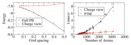
Next we tested the convergence behavior of the pairwise charge-view strategy comparing with the original full PBE for total electrostatic energy calculation. Here we focus on the convergence behavior of the solvation free energy only since it is the component most susceptible to discretization errors. As shown in Fig. 3, the charge-view and the full PBE energies are compared in two different situations: (1) the polarization charges are mapped onto the molecular surface (top) and (2) the polarization charges remain on the grid points. And we also used a nonlinear function y = a + bh^c to fit the convergence data. Thus y|_h=0 is regarded as the “converged” energy. Table 1 shows the fitted coefficients for different strategies. For the original full PBE energies, the convergent value (in kcal/mol) is −7.7915 with relative RMS error of (in kcal/mol) 0.0011.

Figure 3. Convergence of the reaction field energies (kcal/mol) versus grid spacing (Ångstrom).

The AT base dimer was modeled with the full PBE (epsout=80.0, epsin=4.0, istrng=1000). Reaction field energies are computed with the full PBE (black), charge-view (red) strategies. Top: the polarization charges are mapped onto the molecular surface. Bottom: the polarization charges remain on the boundary grid points. For the full PBE and the charge-view methods, the convergence trend lines are fitted with respect to grid spacing in the form of y = a + bx^c. Since the deviation of the field view and charge view without charge mapping (bottom) are large at course grids, only data with grid spacing equal or less than 0.3 Å were used when fitting those curves. See Table 2 for all fitted parameters.

Table 1.

Fitted nonlinear trend lines for the full PBE electrostatic solvation energy (kcal/mol) versus grid spacing using different methods. The nonlinear model to be fitted is y = a + bx^c where x is the grid spacing. RMSrD: root-mean squared relative residue between the fitted values and input values. map: polarization charges are mapped onto the atomic surface. nomap: polarization charges are not mapped onto the atomic surface.

Coefficient	a	b	c	r2	RMSrD
Full PBE	−7.7915	−1.9369	1.4284	0.9966	0.0011
Charge view (map)	−7.7935	0.8683	3.5828	0.9768	0.00062
Charge view (nomap)	−7.7838	−1.6670	1.3078	0.9976	0.00087

In the top figure, the polarization charges are mapped onto the atomic surface, the fitted “converged” energy by the charge-view method is −7.7935 kcal/mol, which is within the RMS error of the converged energy for the full PBE method, indicating that the charge-view method and the full PBE method converge to the same value within fitting uncertainty. In addition, it is apparent that the convergence curve of the charge-view energy is almost flat, indicating that this method offers a good estimation of the full PBE energy at tested coarse grid spacing. This supports our conclusion that the use of polarization charges allows a much faster converging numerical procedure for electrostatic energy calculation as we have shown for the Poisson’s equation and linear PB equation.^{75, 77, 82}

In the bottom figure, the polarization charges are set to remain at the grid points. It can be seen that the fitted “converged” energy by the charge-view method is −7.7838 kcal/mol, which is also within the RMS error of the converged energy for the FDPB method. However, the charge-view energy also converges similarly as the full PBE energy, so that its energy is no longer a good approximation of the converged energy at coarse grid spacing if the polarization charges remain at the grid points.

D. Convergence and treatment of ionic energy terms

The full PBE electrostatic energy is composed of the reaction field energy and the salt-related energy. As discussed in the subsection E of Theory and Computational Details, salt-related energy is only a small portion of the total electrostatic energy and it also converges very rapidly. We studied a typical-sized nucleic acid (PDBID: 420D), a 1026-atom solute. The convergence of salt-related energy of 420D by the full PBE method is shown in Fig. 4. The data was first fitted by nonlinear curve y = a + bh^c, given a predicted energy y=1.865 kcal/mol at h=0, which is less than 10⁻³ of the total electrostatic solvation free energy of 4.7×10³ kcal/mol. Fig. 4 also shows that the salt-related energy converges very well at typical grid spacing values (1/16 to 1/2 Angstrom). The convergence error is <10⁻⁴ of the total electrostatic solvation free energy at grid spacing values less than 1/2 Angstrom and is <10⁻⁵ at grid spacing values less than 1/4 Angstrom.

Figure 4. Convergence of salt-related energy term (kcal/mol) versus grid spacing (Ångstrom).

The nucleic acid 420D was modeled with the full PBE (epsout=80.0, epsin=1.0, istrng=1000). The salt energy is the sum of the ionic energy term and the entropy term in the full PB electrostatic free energy. Top: The salt energy versus grid spacing. The convergence trend lines are fitted with respect to grid spacing in the form of y = a + bx^c. Bottom: The deviation between the salt energies and predicted energy at h=0 according to the curve fitting. The deviation is relative and is respect to predicted total solvation free energy.

On the other hand, as shown in eqn (25), calculation of the ionic energy with the charge view method needs a pair-wise summation of all grid points (N), scaling quadratically with the number of grid points, O(N²), which is very computationally demanding, while the original finite-difference full PBE method (particle mesh) scales only linearly with the number of grid points, O(N). Therefore in the development of an efficient P3M method, the original finite-difference approach is used for the salt-related terms.

E. Accuracy and Efficiency of P3M method

As presented in Theory and Computational Details (subsection D), the essence of the P3M strategy is to use the more accurate charge-based treatments of energy and forces for short-range interactions and keep the long-ranged interactions from the finite-difference full PBE treatment. Our discussion in Theory and Computational Details (subsection E) and the testing data above show that the ionic terms can generally be treated as in the finite-difference full PBE treatment without introducing much error, so the charge-based method is only applied to Coulomb and reaction field interactions to balance accuracy and efficiency.

The pairwise cutoff for the short-range interactions in the P3M strategy apparently influences the accuracy of energy and forces calculation. In general, a larger cutoff leads to more accurate results but is more computationally demanding. Worth noting is that the total electrostatic energy converges very rapidly: the relative error is already less than 10⁻⁴ when a very short cutoff distance of six grids is used. This is already within the convergence errors of the pairwise charge view method at typical coarse grid spacing used, i.e. 1/2 or 1/4 Angstrom as shown in Fig. 3 and Table 1. For example, at 1/4 Angstrom, the charge view energy is −7.7962 kcal/mol, the relative error is 6×10⁻⁴ compares to the fitted value of the full PB equation, the relative error is larger when grid spacing is 1/2 Angstrom.

However the accuracy of atomic forces is more sensitive to cutoff. Table 2 summarizes the accuracy of atomic reaction forces for the tested nucleic acid 420D. The errors in forces by the P3M strategy with different cutoffs were analyzed with the charge-view method set as the benchmark. The grid spacing was set as 1/2 Angstrom and 1/4 Angstrom. It is clear that the errors of forces decrease when the cutoff distance increases. And the force errors at the 1/4 Angstrom grid spacing are also smaller than those at the 1/2 Angstrom grid spacing. In the following analysis, the short-range cutoff distance is set as 14 grid spacing, with which the RMS error of the forces is < 5×10⁻⁴.

Table 2.

Root-mean-squared relative deviations in P3M reaction field forces on DNA 420D with absolute values greater than 1 kcal/mol-Å for the P3M strategy with different cutoff (in grid spacing) compared to the charge view method. Both grid spacing of 0.25 Å and grid spacing of 0.50 Å are computed. Polarization charges are mapped onto the atomic surface.

Cutoff	RMSrD force components (0.50 Å)	RMSrD force components (0.25 Å)
6	2.7×10−3	1.1×10−3
8	1.3×10−3	5.6×10−4
10	9.4×10−4	4.3×10−4
12	6.2×10−4	3.2×10−4
14	4.4×10−4	2.4×10−4
16	3.4×10−4	1.9×10−4

Next the consistency of the P3M method and the pairwise charge-based method was systematically validated with a large set of PDB structures of nucleic acids. Fig. 5 shows the electrostatic energy correlation between the charge view method and the P3M method for non-linear PB equations. It can be seen that these two sets of data are highly consistent with each other, with relative error less than 5×10⁻⁴.

Figure 5. Correlations between full PBE electrostatic energies (kcal/mol) computed by the charge view and the P3M methods.

A test set of 283 different nucleic acids was modeled with the full PBE (epsout=80.0, epsin=4.0, istrng=1000). The charge view energies were computed with the analytical Green’s function, i.e. Coulomb’s law. P3M cutoff is 14. The rms relative deviation is 3.3×10⁻⁴.

Finally a timing analysis was conducted on the tested nucleic acids and is shown in Fig. 6, which plots the correlation of CPU times of energy/force computation versus the system sizes (no. of atoms). It is clear that the P3M time scales with system size much better than the pairwise charge view strategy, with the difference becomes significantly larger when the no. of atoms approaching 1,000’s.

Figure 6. CPU time versus no. of solute atoms for the pairwise charge view method and the P3M method.

The same test set of nucleic acids was modeled with the full PB equation (epsout=80.0, epsin=4.0, istrng=1000) as in Figure 5. The x-axis is the number of atoms in each nucleic acids, the y-axis is the cost of CPU time for computing the energies. The trend lines are fitted functions in the form of y = ax² + bx + c.

F. Accuracy and convergence of electrostatic forces

The accuracy and convergence of electrostatic forces are important issues if we want to use the new method for dynamics simulations. A comparison of the original PBE method, pairwise charge view method, and the P3M method is shown in Fig. 7–Fig. 10 and Table 3–4. We first studied the performance of the new methods with all polarization charges mapped to molecular surface as shown to improve the convergence of energies (Fig. 3).

Figure 7. Self-convergence of reaction field forces (kcal/mol-Å).

The AT base dimer was modeled with the full PBE. (epsout=80.0, epsin=4.0, istrng=1000). Left: field-view method. Center: charge-view method. Right: P3M method. The polarization charges are mapped onto the molecular surface. See Table 4 for correlation analyses.

Figure 10. Consistency of reaction field forces (kcal/mol-Å) among different force interpretation methods at tested fine grid spacing.

Same as Figure 8, except that the polarization charges remain on the boundary grid points. Top: the rms relative deviation is 0.0002. Bottom: the rms relative deviation is 0.0002.

Table 3.

Root-mean-squared relative deviations in reaction field forces with absolute values greater than 1 kcal/mol-Å between strategy y and strategy x. Polarization charges are mapped onto the atomic surface.

x	y	RMSrD
0.0625 full PBE	0.5 full PBE	0.084
0.0625 full PBE	0.25 full PBE	0.038
0.0625 full PBE	0.125 full PBE	0.0092
0.0625 charge view	0.5 charge view	0.025
0.0625 charge view	0.25 charge view	0.0077
0.0625 charge view	0.125 charge view	0.0023
0.0625 P3M	0.5 P3M	0.025
0.0625 P3M	0.25 P3M	0.0076
0.0625 P3M	0.125 P3M	0.0023
0.0625 charge view	0.0625 full PB	0.0053
0.0625 charge view	0.0625 P3M	0.00020

Table 4.

Root-mean-squared relative deviations in reaction field forces with absolute values greater than 1 kcal/mol-Å between strategy y and strategy x. Polarization charges are not mapped onto the atomic surface.

x	y	RMSrD
0.0625 full PBE	0.5 full PBE	0.084
0.0625 full PBE	0.25 full PBE	0.038
0.0625 full PBE	0.125 full PBE	0.0092
0.0625 charge view	0.5 charge view	0.078
0.0625 charge view	0.25 charge view	0.035
0.0625 charge view	0.125 charge view	0.0090
0.0625 P3M	0.5 P3M	0.077
0.0625 P3M	0.25 P3M	0.035
0.0625 P3M	0.125 P3M	0.0092
0.0625 charge view	0.0625 full PB	0.00024
0.0625 charge view	0.0625 P3M	0.00024

Fig. 7 plots the correlations of forces computed at different grid spacing values with the benchmark data set obtained at the finest grid spacing used (1/16 Angstrom). It is clear that the correlation becomes better as the grid spacing decreases. Table 3 shows the RMS relative errors for the dominant force components (here chosen to be larger than 1 kcal/mol-Å) at tested grid spacing values with respect to the benchmark data set. The analysis shows that the RMS relative error becomes significantly smaller for all three tested strategies as the grid spacing is reduced. As the grid spacing reduces from 0.5 Angstrom to 0.125 Angstrom, the RMS relative error for the original full PB method is reduced from 0.084 to 0.0092, while for the charge view method and P3M method, the error is reduced from 0.025 to 0.0023. It is also interesting to notice that the RMS relative errors of the both the charge-view method and the P3M method are significantly smaller than those of the original finite-difference method at all tested grid spacing values (1/8 to 1/2 Angstrom). Finally, the consistency among the three different methods at 1/16 Angstroms is also shown in Fig. 8 and Table 3. The RMS relative error between the charge view method and the full PBE method is 0.0053. This is similar to the convergence error of the full PBE energy (Fig. 3) at 1/16 Angstrom, around 0.0047, assuming the charge-view method converges much earlier as shown in Fig. 3 (top panel). The RMS relative error between the charge view method and the P3M method is 0.0002, which is consistent with the accuracy of the P3M method for energies as shown in Fig. 5.

Figure 8. Consistency of reaction field forces (kcal/mol-Å) among different force interpretation methods at the tested fine grid spacing.

Polarization charges are mapped onto the molecular surface. (epsout=80.0, epsin=4.0, istrng=1000). Top: The full PBE versus charge view. The rms relative deviation is 0.0052 for nontrivial force components (absolute values > 1 kcal/mol-Å). Bottom: P3M versus charge view. The rms relative deviation is 0.0002 for nontrivial force components. The fine grid spacing is set at 1/16 Angstrom as in Figure 7.

In Fig. 9 and 10 and Table 4 the same analysis was conducted but with the polarization charges set to remain on the grid points for charge-view and P3M methods. Fig. 9 shows that the correlation becomes better as the grid spacing decreases, similar to Fig. 7. Table 4 shows that for the charge view method and P3M method, the RMS relative errors at all grid spacing values are larger than those with the polarization charges mapped onto the molecular surface (Table 3). Table 4 also shows that the consistency among the three methods is higher at the finest grid spacing (1/16 Angstrom) when charges are set to remain at the grid points. This is also in agreement with the convergence trend of energies as presented in Fig. 3 (bottom panel). Note too the benefits of mapping charges remain to be high at finer grid spacing tested, i.e. 1/4 and 1/8 Angstrom. In summary the two sets of convergence data support the practice of mapping polarization charges onto the molecular surface.

Figure 9. Self-convergence of reaction field forces (kcal/mol-Å).

Same as Figure 7, except that the polarization charges remain on the boundary grid points. See Table 5 for correlation analyses.

G. Net force analysis

In molecular dynamics simulation, the net system force is supposed to be zero given the use of a conservative force field. However, due to numerical error, the net force is in general not zero. Thus this is a simple initial test to assess whether the force interpolation is accurate enough before it is tested in the complex molecular dynamics programs.

Here the analysis was conducted on the 1026-atom nucleic acid (420D) and also a 1389-atom protein (1F81), to demonstrate the performance of the P3M method. As shown in Table 5, the net force is first computed and averaged over each atom, and then the unsigned average of the force components over all the atoms are also computed as references. As shown in Table 5, the averaged net force components are always less than 10⁻³ of the unsigned average force components. This should be viewed in the context of typical continuum dynamics simulations, where Langevin thermostat is often used. Given a small collision frequency (1 ps⁻¹) often used in continuum dynamics simulations, a time step of 0.001 ps, and 300K simulation temperature, the average random forces are ~1.7 kcal/mol-Å on the lightest hydrogen atoms. Thus the nonzero net force plays a less significant role in biasing the dynamics simulations.

Table 5.

Averaged net force and unsigned average of force components in x, y, z directions for nucleic acid 420D and protein 1F81. The unit is kcal/mol-Å.

Biomolecules	420D	1F81
Average net force x	−3.2×10−4	−2.1×10−4
Average unsigned force x	3.4	2.5
Average net force y	−6.2×10−4	−7.7×10−4
Average unsigned force y	3.7	2.5
Average net force z	−9.1×10−4	−9.3×10−5
Average unsigned force z	2.7	2.5

Conclusions

In this work, we proposed a charge-central interpretation of the full nonlinear PBE electrostatic interactions. The validity of this charge-view framework, formulated as a vacuum Poisson equation with effective charges, was first demonstrated by reproducing the electrostatic potentials of the original solvated full nonlinear PBE for a tested DNA molecule with or without salt. In addition the full nonlinear PB electrostatics energy can be reproduced by the pairwise summation of effective charges within the charge-view framework for a large set of tested biomolecules. Finally, the energy convergence analyses show the use of polarization charges allows a much faster converging numerical procedure for electrostatic energy calculation as we have shown for the Poisson’s equation and linear PB equation.

Given the validity of the charge-view framework, we went ahead to propose a full particle-particle particle-mesh treatment for the total electrostatic interactions of full nonlinear PB systems. It is interesting to note that salt-related term is only a small portion of the total electrostatic energy and it also converges very rapidly, with convergence error less than 10⁻⁴ of the total electrostatic free energy at typical grid spacing used for biomolecular applications. This allows us to use the relatively more efficient particle-mesh, i.e. the finite-difference approach, to handle the salt-related terms. We also studied the influence of pairwise cutoff for the short-range interactions in the P3M strategy on the accuracy of energy and forces calculation. In general, a cutoff of 14 grid points can be used to achieve a good balance of accuracy and efficiency, with relative error less than 5×10⁻⁴ with respect to the pure particle-particle based charge-view method. Finally, we analyzed the accuracy and the convergence trend of numerical solvation forces with the P3M strategy. Our analysis shows that the P3M method can reproduce charge-view method well at all tested typical grid spacing values (1/16 to 1/2 Angstrom). In addition both the charge-view and P3M method deliver faster-converging forces with reducing grid spacing. The convergence tests also show that the forces computed by the P3M method, the pairwise charge view method, and the original full nonlinear PB method all converge to the consistent values as grid spacing decreases, demonstrating their mutual consistency.

Given the developments and validations documented here, we are working to adapt the P3M treatment of the full nonlinear PB model to molecular dynamics simulations. To support our ongoing development, we also conducted preliminary analysis to assess the feasibility of the numerical strategy presented here by first analyzing the net system force of the tested nontrivial systems. It is widely known that the net numerical force is in general not zero in the numerical methods due to intrinsic numerical errors. Our tests show that the averaged net force components are always less than 10⁻³ of average atomic force components, and also much smaller than the average atomic random forces on the lightest hydrogen atoms in the widely used Langevin thermo bath, indicating that the influence of error of numerical force is small. Apparently efficiency is also an important issue and we are also working to port the new method to the GPU platforms to further study the effect of the nonlinear PB modeling on nontrivial biomolecular problems.

Appendices

A. Effective charge interpretation of Poisson-Boltzmann equation

Before exploring the general Poisson-Boltzmann’s equation, it is instructive to discuss the more fundamental Poisson’s equation

$$\nabla •(\epsilon \nabla \varphi )=-4\pi {\rho }^f$$ (42)

It is well known that ϕ can be split into Coulombic potential and reaction field potential, i.e., ϕ = ϕ_C +ϕ_RF in eqn (42). To see how this is possible, suppose a solute molecule with dielectric constant ε_i is surrounded by a solvent medium with a uniform dielectric constant ε_o, the Coulombic potential is defined as

$${\epsilon }_i{\nabla }^2{\varphi }_C=-4\pi {\rho }^f$$ (43)

which means that the Coulombic potential (ϕ_C) is generated by atomic charges in a uniform medium with dielectric constant ε_i throughout the whole space. Next introduce its associated electric displacement D_C = −ε_i∇ϕ_C = ε_iE_C. Given D_C = E_C + 4πP_C, where P_C is the polarization vector in the uniform dielectric of ε_i. It is clear that eqn (43) can be rewritten as

$$\nabla •{\mathbf{E}}_C+4\pi \nabla •{\mathbf{P}}_C=4\pi {\rho }^f$$ (44)

With the Coulombic field (E_C) so defined, the reaction field is simply the electrostatic field generated by the charges induced by transferring the environment surrounding the solute from ε_o to ε_i. To obtain an equation for the reaction field potential, we first reformulate eqn (42) with the help of the electric displacement vector for the inhomogeneous dielectric D = −ε∇ϕ = εE

$$\nabla •(\epsilon \mathbf{E})=\nabla •\mathbf{D}=4\pi {\rho }^f$$ (45)

Now define E_RF and P_RF so that they satisfy the following relation between the total electrostatic field/polarization and the Coulombic field/polarization:

$$\begin{array}{l}\mathbf{E}={\mathbf{E}}_C+{\mathbf{E}}_{RF}\\ \mathbf{P}={\mathbf{P}}_C+{\mathbf{P}}_{RF}\end{array}$$ (46)

Thus E_RF and P_RF are the reaction field and polarization, respectively, induced by the inhomogeneous dielectric with respect to the homogeneous dielectric as in eqn (44). Substitution of D = E+ 4πP into eqn (42), we have

$$\nabla •{\mathbf{E}}_C+\nabla •{\mathbf{E}}_{RF}+4\pi \nabla •{\mathbf{P}}_C+4\pi \nabla •{\mathbf{P}}_{RF}=4\pi {\rho }^f$$ (47)

Given eqn (47), it can be simplified to

$$\nabla •{\mathbf{E}}_{RF}=-4\pi \nabla •{\mathbf{P}}_{RF}$$ (48)

Thus the reaction field potential satisfies

$$\begin{array}{l}{\nabla }^2{\varphi }_{RF}=\nabla •{\mathbf{E}}_{RF}=-4\pi {\rho }^{\mathit{pol}}\\ \text{Given}{\rho }^{\mathit{pol}}=-\nabla •{\mathbf{P}}_{RF}\end{array}$$ (49)

Given ϕ = ϕ_C + ϕ_RF and eqn (43) and (49), the Poisson’s eqn (42) can then be reformulated as

$${\nabla }^2\varphi =-4\pi \left(\frac{{\rho }^f}{{\epsilon }_i}+{\rho }^{\mathit{pol}}\right)$$ (50)

Thus the total electrostatic potential can be viewed as the summation of two vacuum Coulombic potentials: ϕ_C from effective charge source $\frac{{\rho }^f}{{\epsilon }_i}$ and reaction field potential ϕ_RF from effective charge source ρ^pol. In reformulating the Poisson’s equation this way, it is possible to explore alternative strategies in solving the equation. Of course, this requires an efficient way to compute the polarization charges, for example, as shown in one of our recent works.⁹⁴

Now consider the more general Poisson-Boltzmann equation for systems with continuum mobile ions

$$\nabla •(\epsilon \nabla \varphi )=-4\pi {\rho }^f-4\pi \sum _i{e}_i{c}_{i}exp(-e_i\varphi /k_{B}T)\lambda$$ (51)

where e_i is the charge of ion type i, c_i is the bulk number density of ion type i, λ is the ion exclusion function, k_B is the Boltzmann constant and T is the absolute temperature. Following the development in the Poisson’s equation, what is needed here is a decomposition of total electrostatic potential when the continuum ion terms present.

To build upon the previous analysis of Poisson’s equation, let us assume that the final state of the system is reached first by charging up the solute without any continuum ions, then by releasing the continuum ions. Thus, the final electrostatic potential for the Poisson-Boltzmann’s equation (ϕ) can be regarded as a perturbation to the electrostatic potential for the Poisson’s equation (ϕ^PE), i.e. ϕ =ϕ^PE + ϕ^m, where ϕ^m is used to denote the perturbation due to the continuum ions. It is straightforward to show that ϕ^m satisfies the following equation

$$\begin{array}{l}\nabla •(\epsilon \nabla {\varphi }^m)=-4\pi {\rho }^m\\ \text{given}{\rho }^m=\sum _i{e}_i{c}_{i}exp\left(-e_i\varphi /k_{B}T\right)\lambda \end{array}$$ (52)

by substituting ϕ = ϕ^PE + ϕ ^m into the Poisson-Boltzmann’s equation. eqn shows that ϕ^m can be viewed as a potential caused by the charge distribution ρ^m in the dielectric environment just as ϕ^PE is caused by ρ^f in the same dielectric environment.

Similar to the treatment of potential by ρ^f, we shall decompose ρ^m into a Coulombic field and reaction field, ${\varphi }^m={\varphi }_C^m+{\varphi }_{RF}^m$. However, the difference from ρ^f is that ρ^m is immersed in the homogenous dielectric of solvent (ε_o), but not that of solute (ε_i). Therefore the equation for ${\varphi }_C^m$is

$${\epsilon }_o{\nabla }^2{\varphi }_C^m=-{\epsilon }_o\nabla •{\mathbf{E}}_C^m=-4\pi {\rho }^m$$ (53)

Similar to ϕ_RF, ${\varphi }_{RF}^m$ can be viewed as generated by a polarization charge density, ρ^pol,m.

$$\begin{array}{l}{\nabla }^2{\varphi }_{RF}^m=-4\pi {\rho }^{\mathit{pol},m}\\ {\rho }^{\mathit{pol},m}=-\nabla •{\mathbf{P}}_{RF}^m\end{array}$$ (54)

Therefore the perturbation potential ${\varphi }^m={\varphi }_C^m+{\varphi }_{RF}^m$ due to the continuum ions can be regarded as being caused by the charge distributions of $\frac{{\rho }^m}{{\epsilon }_o}$ and ρ^pol,m

$${\nabla }^2{\varphi }^m=-4\pi \left(\frac{{\rho }^m}{{\epsilon }_o}+{\rho }^{\mathit{pol},m}\right),$$ (55)

Now it is time to merge what we have derived in the treatment of Poisson’s equation and the perturbation due to the continuum ions. eqn (51) and (55) thus give us

$${\nabla }^2\varphi =-4\pi \left(\frac{{\rho }^f}{{\epsilon }_i}+\frac{{\rho }^m}{{\epsilon }_o}+{\rho }^{\mathit{pol}}\right),$$ (56)

where we have merged ρ^pol,m into ρ^pol. Here ϕ_RF satisfies the revised relation

$${\nabla }^2{\varphi }_{RF}=-\nabla •{\mathbf{E}}_{RF}=-4\pi {\rho }^{\mathit{pol}}$$

B. High precision finite-difference Green’s function values

The finite-difference Green’s function needed for self-energy and short-range Coulombic energy was previously precomputed based on the work of Luty and McCammon.⁸⁷ Due to limited computational resources, only function values up to 20-grid separation in each dimension were precomputed. In this study, finite-difference Green’s function values were computed in a brute-force manner by solving a vacuum Coulomb field of a point charge of 1 unit charge with the standard finite-difference method. The charge was positioned at the center of the finite-difference grids, and the boundary potential was set analytically according to the Coulomb law. As the grid dimension increases, potentials on grid nodes close to the center converge to the values of the finite-difference Green’s function. Table A.1 shows the maximum relative error of Green’s function as the grid dimension increases. The error analysis shows that 8 digits of accuracy can be achieved when Δx,Δy,Δz ≤ 20, and the error of the function values when Δx,Δy,Δz ≤ 40 is also very close, less than 1.4×10⁻⁸.

The updated finite difference Green’s function values along with the documented algorithms are incorporated in the latest Amber simulation package to be released in the spring of 2016.

Table A.1.

Maximum convergence error of finite-difference Green’s function values when Δx, Δy, Δz ≤ 40 or Δx, Δy, Δz ≤ 20.

Grid dimension	Max error (Δx,Δy,Δz ≤ 40)	Max error (Δx,Δy,Δz ≤ 20)
481×481×481	1.1×10−7	5.7×10−8
601×601×601	5.1×10−8	2.5×10−8
721×721×721	2.6×10−8	1.3×10−8
841×841×841	1.4×10−8	7.3×10−9
961×961×961	NA	NA

References

- 1.Davis ME, Mccammon JA. Electrostatics in Biomolecular Structure and Dynamics. Chem Rev. 1990;90:509–521. [Google Scholar]
- 2.Honig B, Sharp K, Yang AS. Macroscopic Models of Aqueous-Solutions - Biological and Chemical Applications. J Phys Chem. 1993;97:1101–1109. [Google Scholar]
- 3.Honig B, Nicholls A. Classical Electrostatics in Biology and Chemistry. Science. 1995;268:1144–1149. doi: 10.1126/science.7761829. [DOI] [PubMed] [Google Scholar]
- 4.Beglov D, Roux B. Solvation of Complex Molecules in a Polar Liquid: An Integral Equation Theory. J Chem Phys. 1996;104:8678–8689. [Google Scholar]
- 5.Cramer CJ, Truhlar DG. Implicit Solvation Models: Equilibria, Structure, Spectra, and Dynamics. Chem Rev. 1999;99:2161–2200. doi: 10.1021/cr960149m. [DOI] [PubMed] [Google Scholar]
- 6.Bashford D, Case DA. Generalized Born Models of Macromolecular Solvation Effects. Annu Rev Phys Chem. 2000;51:129–152. doi: 10.1146/annurev.physchem.51.1.129. [DOI] [PubMed] [Google Scholar]
- 7.Baker NA. Improving Implicit Solvent Simulations: A Poisson-Centric View. Curr Opin Struct Biol. 2005;15:137–143. doi: 10.1016/j.sbi.2005.02.001. [DOI] [PubMed] [Google Scholar]
- 8.Chen JH, Im WP, Brooks CL. Balancing Solvation and Intramolecular Interactions: Toward a Consistent Generalized Born Force Field. J Am Chem Soc. 2006;128:3728–3736. doi: 10.1021/ja057216r. [DOI] [PMC free article] [PubMed] [Google Scholar]
- 9.Feig M, Chocholousova J, Tanizaki S. Extending the Horizon: Towards the Efficient Modeling of Large Biomolecular Complexes in Atomic Detail. Theor Chem Acc. 2006;116:194–205. [Google Scholar]
- 10.Koehl P. Electrostatics Calculations: Latest Methodological Advances. Curr Opin Struct Biol. 2006;16:142–151. doi: 10.1016/j.sbi.2006.03.001. [DOI] [PubMed] [Google Scholar]
- 11.Im W, Chen JH, Brooks CL. Peptide and Protein Folding and Conformational Equilibria: Theoretical Treatment of Electrostatics and Hydrogen Bonding with Implicit Solvent Models. Peptide Solvation and H-Bonds. 2006;72:173–98. doi: 10.1016/S0065-3233(05)72007-6. [DOI] [PubMed] [Google Scholar]
- 12.Lu BZ, Zhou YC, Holst MJ, Mccammon JA. Recent Progress in Numerical Methods for the Poisson-Boltzmann Equation in Biophysical Applications. Commun Comput Phys. 2008;3:973–1009. [Google Scholar]
- 13.Wang J, Tan CH, Tan YH, Lu Q, Luo R. Poisson-Boltzmann Solvents in Molecular Dynamics Simulations. Commun Comput Phys. 2008;3:1010–1031. [Google Scholar]
- 14.Altman MD, Bardhan JP, White JK, Tidor B. Accurate Solution of Multi-Region Continuum Biomolecule Electrostatic Problems Using the Linearized Poisson-Boltzmann Equation with Curved Boundary Elements. J Comput Chem. 2009;30:132–153. doi: 10.1002/jcc.21027. [DOI] [PMC free article] [PubMed] [Google Scholar]
- 15.Chen Z, Baker NA, Wei GW. Differential Geometry Based Solvation Model I: Eulerian Formulation. J Comput Phys. 2010;229:8231–8258. doi: 10.1016/j.jcp.2010.06.036. [DOI] [PMC free article] [PubMed] [Google Scholar]
- 16.Xiao TJ, Song XY. A Molecular Debye-Huckel Theory and Its Applications to Electrolyte Solutions. J Chem Phys. 2011;135:104104. doi: 10.1063/1.3632052. [DOI] [PubMed] [Google Scholar]
- 17.Cai Q, Wang J, Hsieh M-J, Ye X, Luo R. Chapter Six - Poisson–Boltzmann Implicit Solvation Models. In: Ralph AW, editor. Annual Reports in Computational Chemistry. Vol. 8. Elsevier; 2012. pp. 149–162. [Google Scholar]
- 18.Botello-Smith WM, Cai Q, Luo R. Biological Applications of Classical Electrostatics Methods. J Chem Theory Comput. 2014;13:1440008. [Google Scholar]
- 19.Fogolari F, Brigo A, Molinari H. The Poisson-Boltzmann Equation for Biomolecular Electrostatics: A Tool for Structural Biology. J Mol Recognit. 2002;15:377–392. doi: 10.1002/jmr.577. [DOI] [PubMed] [Google Scholar]
- 20.Lwin TZ, Zhou RH, Luo R. Is Poisson-Boltzmann Theory Insufficient for Protein Folding Simulations? J Chem Phys. 2006;124:034902. doi: 10.1063/1.2161202. [DOI] [PubMed] [Google Scholar]
- 21.Warwicker J, Watson HC. Calculation of the Electric-Potential in the Active-Site Cleft Due to Alpha-Helix Dipoles. J Mol Biol. 1982;157:671–679. doi: 10.1016/0022-2836(82)90505-8. [DOI] [PubMed] [Google Scholar]
- 22.Bashford D, Karplus M. Pkas of Ionizable Groups in Proteins - Atomic Detail from a Continuum Electrostatic Model. Biochemistry. 1990;29:10219–10225. doi: 10.1021/bi00496a010. [DOI] [PubMed] [Google Scholar]
- 23.Sharp KA, Honig B. Electrostatic Interactions in Macromolecules - Theory and Applications. Annu Rev Biophys Biomol Struct. 1990;19:301–332. doi: 10.1146/annurev.bb.19.060190.001505. [DOI] [PubMed] [Google Scholar]
- 24.Jeancharles A, Nicholls A, Sharp K, Honig B, Tempczyk A, Hendrickson TF, Still WC. Electrostatic Contributions to Solvation Energies - Comparison of Free-Energy Perturbation and Continuum Calculations. J Am Chem Soc. 1991;113:1454–1455. [Google Scholar]
- 25.Gilson MK. Theory of Electrostatic Interactions in Macromolecules. Curr Opin Struct Biol. 1995;5:216–223. doi: 10.1016/0959-440x(95)80079-4. [DOI] [PubMed] [Google Scholar]
- 26.Edinger SR, Cortis C, Shenkin PS, Friesner RA. Solvation Free Energies of Peptides: Comparison of Approximate Continuum Solvation Models with Accurate Solution of the Poisson-Boltzmann Equation. J Phys Chem B. 1997;101:1190–1197. [Google Scholar]
- 27.Klapper I, Hagstrom R, Fine R, Sharp K, Honig B. Focusing of Electric Fields in the Active Site of Copper-Zinc Superoxide Dismutase Effects of Ionic Strength and Amino Acid Modification. PROTEINS. 1986;1:47–59. doi: 10.1002/prot.340010109. [DOI] [PubMed] [Google Scholar]
- 28.Davis ME, Mccammon JA. Solving the Finite-Difference Linearized Poisson-Boltzmann Equation - a Comparison of Relaxation and Conjugate-Gradient Methods. J Comput Chem. 1989;10:386–391. [Google Scholar]
- 29.Nicholls A, Honig B. A Rapid Finite-Difference Algorithm, Utilizing Successive over-Relaxation to Solve the Poisson-Boltzmann Equation. J Comput Chem. 1991;12:435–445. [Google Scholar]
- 30.Luty BA, Davis ME, Mccammon JA. Solving the Finite-Difference Nonlinear Poisson-Boltzmann Equation. J Comput Chem. 1992;13:1114–1118. [Google Scholar]
- 31.Holst M, Saied F. Multigrid Solution of the Poisson-Boltzmann Equation. J Comput Chem. 1993;14:105–113. [Google Scholar]
- 32.Forsten KE, Kozack RE, Lauffenburger DA, Subramaniam S. Numerical-Solution of the Nonlinear Poisson-Boltzmann Equation for a Membrane-Electrolyte System. J Phys Chem. 1994;98:5580–5586. [Google Scholar]
- 33.Holst MJ, Saied F. Numerical-Solution of the Nonlinear Poisson-Boltzmann Equation-Developing More Robust and Efficient Methods. J Comput Chem. 1995;16:337–364. [Google Scholar]
- 34.Bashford D. An Object-Oriented Programming Suite for Electrostatic Effects in Biological Molecules. Lecture Notes in Comput Sci. 1997;1343:233–240. [Google Scholar]
- 35.Im W, Beglov D, Roux B. Continuum Solvation Model: Computation of Electrostatic Forces from Numerical Solutions to the Poisson-Boltzmann Equation. Comput Phys Commun. 1998;111:59–75. [Google Scholar]
- 36.Wang J, Luo R. Assessment of Linear Finite-Difference Poisson-Boltzmann Solvers. J Comput Chem. 2010;31:1689–1698. doi: 10.1002/jcc.21456. [DOI] [PMC free article] [PubMed] [Google Scholar]
- 37.Cai Q, Hsieh M-J, Wang J, Luo R. Performance of Nonlinear Finite-Difference Poisson-Boltzmann Solvers. J Chem Theory Comput. 2010;6:203–211. doi: 10.1021/ct900381r. [DOI] [PMC free article] [PubMed] [Google Scholar]
- 38.Rocchia W, Alexov E, Honig B. Extending the Applicability of the Nonlinear Poisson-Boltzmann Equation: Multiple Dielectric Constants and Multivalent Ions. J Phys Chem B. 2001;105:6507–6514. [Google Scholar]
- 39.Luo R, David L, Gilson MK. Accelerated Poisson-Boltzmann Calculations for Static and Dynamic Systems. J Comput Chem. 2002;23:1244–1253. doi: 10.1002/jcc.10120. [DOI] [PubMed] [Google Scholar]
- 40.Cai Q, Wang J, Zhao H-K, Luo R. On Removal of Charge Singularity in Poisson-Boltzmann Equation. J Chem Phys. 2009;130:145101. doi: 10.1063/1.3099708. [DOI] [PubMed] [Google Scholar]
- 41.Wang J, Cai Q, Li Z-L, Zhao H-K, Luo R. Achieving Energy Conservation in Poisson-Boltzmann Molecular Dynamics: Accuracy and Precision with Finite-Difference Algorithms. Chem Phys Lett. 2009;468:112–118. doi: 10.1016/j.cplett.2008.12.049. [DOI] [PMC free article] [PubMed] [Google Scholar]
- 42.Botello-Smith WM, Liu X, Cai Q, Li Z, Zhao H, Luo R. Numerical Poisson-Boltzmann Model for Continuum Membrane Systems. Chem Phys Lett. 2012:274–281. doi: 10.1016/j.cplett.2012.10.081. [DOI] [PMC free article] [PubMed] [Google Scholar]
- 43.Cortis CM, Friesner RA. Numerical Solution of the Poisson-Boltzmann Equation Using Tetrahedral Finite-Element Meshes. J Comput Chem. 1997;18:1591–1608. [Google Scholar]
- 44.Holst M, Baker N, Wang F. Adaptive Multilevel Finite Element Solution of the Poisson-Boltzmann Equation I. Algorithms and Examples. J Comput Chem. 2000;21:1319–1342. [Google Scholar]
- 45.Baker N, Holst M, Wang F. Adaptive Multilevel Finite Element Solution of the Poisson-Boltzmann Equation Ii. Refinement at Solvent-Accessible Surfaces in Biomolecular Systems. J Comput Chem. 2000;21:1343–1352. [Google Scholar]
- 46.Shestakov AI, Milovich JL, Noy A. Solution of the Nonlinear Poisson-Boltzmann Equation Using Pseudo-Transient Continuation and the Finite Element Method. J Colloid Interface Sci. 2002;247:62–79. doi: 10.1006/jcis.2001.8033. [DOI] [PubMed] [Google Scholar]
- 47.Chen L, Holst MJ, Xu JC. The Finite Element Approximation of the Nonlinear Poisson-Boltzmann Equation. Siam J Numer Anal. 2007;45:2298–2320. [Google Scholar]
- 48.Xie D, Zhou S. A New Minimization Protocol for Solving Nonlinear Poisson–Boltzmann Mortar Finite Element Equation. BIT Numer Math. 2007;47:853–871. [Google Scholar]
- 49.Lu B, Zhou YC. Poisson-Nernst-Planck Equations for Simulating Biomolecular Diffusion-Reaction Processes Ii: Size Effects on Ionic Distributions and Diffusion-Reaction Rates. Biophys J. 2011;100:2475–2485. doi: 10.1016/j.bpj.2011.03.059. [DOI] [PMC free article] [PubMed] [Google Scholar]
- 50.Lu B, Holst MJ, Mccammon JA, Zhou YC. Poisson-Nernst-Planck Equations for Simulating Biomolecular Diffusion-Reaction Processes I: Finite Element Solutions. J Comput Phys. 2010;229:6979–6994. doi: 10.1016/j.jcp.2010.05.035. [DOI] [PMC free article] [PubMed] [Google Scholar]
- 51.Bond SD, Chaudhry JH, Cyr EC, Olson LN. A First-Order System Least-Squares Finite Element Method for the Poisson-Boltzmann Equation. J Comput Chem. 2010;31:1625–1635. doi: 10.1002/jcc.21446. [DOI] [PubMed] [Google Scholar]
- 52.Miertus S, Scrocco E, Tomasi J. Electrostatic Interaction of a Solute with a Continuum - a Direct Utilization of Abinitio Molecular Potentials for the Prevision of Solvent Effects. Chemical Physics. 1981;55:117–129. [Google Scholar]
- 53.Hoshi H, Sakurai M, Inoue Y, Chujo R. Medium Effects on the Molecular Electronic-Structure.1. The Formulation of a Theory for the Estimation of a Molecular Electronic-Structure Surrounded by an Anisotropic Medium. J Chem Phys. 1987;87:1107–1115. [Google Scholar]
- 54.Zauhar RJ, Morgan RS. The Rigorous Computation of the Molecular Electric-Potential. J Comput Chem. 1988;9:171–187. [Google Scholar]
- 55.Rashin AA. Hydration Phenomena, Classical Electrostatics, and the Boundary Element Method. J Phys Chem. 1990;94:1725–1733. [Google Scholar]
- 56.Yoon BJ, Lenhoff AM. A Boundary Element Method for Molecular Electrostatics with Electrolyte Effects. J Comput Chem. 1990;11:1080–1086. [Google Scholar]
- 57.Juffer AH, Botta EFF, Vankeulen BaM, Vanderploeg A, Berendsen HJC. The Electric-Potential of a Macromolecule in a Solvent - a Fundamental Approach. J Comput Phys. 1991;97:144–171. [Google Scholar]
- 58.Zhou HX. Boundary-Element Solution of Macromolecular Electrostatics - Interaction Energy between 2 Proteins. Biophys J. 1993;65:955–963. doi: 10.1016/S0006-3495(93)81094-4. [DOI] [PMC free article] [PubMed] [Google Scholar]
- 59.Bharadwaj R, Windemuth A, Sridharan S, Honig B, Nicholls A. The Fast Multipole Boundary-Element Method for Molecular Electrostatics - an Optimal Approach for Large Systems. J Comput Chem. 1995;16:898–913. [Google Scholar]
- 60.Purisima EO, Nilar SH. A Simple yet Accurate Boundary-Element Method for Continuum Dielectric Calculations. J Comput Chem. 1995;16:681–689. [Google Scholar]
- 61.Liang J, Subramaniam S. Computation of Molecular Electrostatics with Boundary Element Methods. Biophys J. 1997;73:1830–1841. doi: 10.1016/S0006-3495(97)78213-4. [DOI] [PMC free article] [PubMed] [Google Scholar]
- 62.Vorobjev YN, Scheraga HA. A Fast Adaptive Multigrid Boundary Element Method for Macromolecular Electrostatic Computations in a Solvent. J Comput Chem. 1997;18:569–583. [Google Scholar]
- 63.Totrov M, Abagyan R. Rapid Boundary Element Solvation Electrostatics Calculations in Folding Simulations: Successful Folding of a 23-Residue Peptide. Biopolymers. 2001;60:124–133. doi: 10.1002/1097-0282(2001)60:2<124::AID-BIP1008>3.0.CO;2-S. [DOI] [PubMed] [Google Scholar]
- 64.Boschitsch AH, Fenley MO, Zhou HX. Fast Boundary Element Method for the Linear Poisson-Boltzmann Equation. J Phys Chem B. 2002;106:2741–2754. [Google Scholar]
- 65.Lu BZ, Cheng XL, Huang JF, Mccammon JA. Order N Algorithm for Computation of Electrostatic Interactions in Biomolecular Systems. Proc Natl Acad Sci USA. 2006;103:19314–19319. doi: 10.1073/pnas.0605166103. [DOI] [PMC free article] [PubMed] [Google Scholar]
- 66.Lu B, Cheng X, Huang J, Mccammon JA. An Adaptive Fast Multipole Boundary Element Method for Poisson-Boltzmann Electrostatics. J Chem Theory Comput. 2009;5:1692–1699. doi: 10.1021/ct900083k. [DOI] [PMC free article] [PubMed] [Google Scholar]
- 67.Bajaj C, Chen S-C, Rand A. An Efficient Higher-Order Fast Multipole Boundary Element Solution for Poisson-Boltzmann-Based Molecular Electrostatics. Siam J Sci Comput. 2011;33:826–848. doi: 10.1137/090764645. [DOI] [PMC free article] [PubMed] [Google Scholar]
- 68.Bardhan JP. Numerical Solution of Boundary-Integral Equations for Molecular Electrostatics. J Chem Phys. 2009;130:094102. doi: 10.1063/1.3080769. [DOI] [PubMed] [Google Scholar]
- 69.Davis ME, Mccammon JA. Calculating Electrostatic Forces from Grid-Calculated Potentials. J Comput Chem. 1990;11:401–409. [Google Scholar]
- 70.Sharp K. Incorporating Solvent and Ion Screening into Molecular-Dynamics Using the Finite-Difference Poisson-Boltzmann Method. J Comput Chem. 1991;12:454–468. [Google Scholar]
- 71.Zauhar RJ. The Incorporation of Hydration Forces Determined by Continuum Electrostatics into Molecular Mechanics Simulations. J Comput Chem. 1991;12:575–583. [Google Scholar]
- 72.Niedermeier C, Schulten K. Molecular-Dynamics Simulations in Heterogeneous Dielectrica and Debye-Huckel Media - Application to the Protein Bovine Pancreatic Trypsin-Inhibitor. Mol Simul. 1992;8:361–387. [Google Scholar]
- 73.Gilson MK, Davis ME, Luty BA, Mccammon JA. Computation of Electrostatic Forces on Solvated Molecules Using the Poisson-Boltzmann Equation. J Phys Chem. 1993;97:3591–3600. [Google Scholar]
- 74.Che J, Dzubiella J, Li B, Mccammon JA. Electrostatic Free Energy and Its Variations in Implicit Solvent Models. J Phys Chem B. 2008;112:3058–3069. doi: 10.1021/jp7101012. [DOI] [PubMed] [Google Scholar]
- 75.Cai Q, Ye X, Wang J, Luo R. Dielectric Boundary Force in Numerical Poisson-Boltzmann Methods: Theory and Numerical Strategies. Chem Phys Lett. 2011;514:368–373. doi: 10.1016/j.cplett.2011.08.067. [DOI] [PMC free article] [PubMed] [Google Scholar]
- 76.Li B, Cheng X, Zhang Z. Dielectric Boundary Force in Molecular Solvation with the Poisson-Boltzmann Free Energy: A Shape Derivative Approach. Siam J Appl Math. 2011;71:2093–2111. doi: 10.1137/110826436. [DOI] [PMC free article] [PubMed] [Google Scholar]
- 77.Cai Q, Ye X, Luo R. Dielectric Pressure in Continuum Electrostatic Solvation of Biomolecules. Phys Chem Chem Phys. 2012;14:15917–15925. doi: 10.1039/c2cp43237d. [DOI] [PMC free article] [PubMed] [Google Scholar]
- 78.Xiao L, Wang CH, Luo R. Recent Progress in Adapting Poisson-Boltzmann Methods to Molecular Simulations. J Theor Comput Chem. 2014;13:1430001. [Google Scholar]
- 79.Xiao L, Cai Q, Ye X, Wang J, Luo R. Electrostatic Forces in the Poisson-Boltzmann Systems. J Chem Phys. 2013;139:094106. doi: 10.1063/1.4819471. [DOI] [PMC free article] [PubMed] [Google Scholar]
- 80.Davis ME, Mccammon JA. Dielectric Boundary Smoothing in Finite-Difference Solutions of the Poisson Equation - an Approach to Improve Accuracy and Convergence. J Comput Chem. 1991;12:909–912. [Google Scholar]
- 81.Bruccoleri RE. Grid Positioning Independence and the Reduction of Self-Energy in the Solution of the Poisson-Boltzmann Equation. J Comput Chem. 1993;14:1417–1422. [Google Scholar]
- 82.Wang J, Cai Q, Xiang Y, Luo R. Reducing Grid Dependence in Finite-Difference Poisson-Boltzmann Calculations. J Chem Theory Comput. 2012;8:2741–2751. doi: 10.1021/ct300341d. [DOI] [PMC free article] [PubMed] [Google Scholar]
- 83.Zauhar RJ, Morgan RS. A New Method for Computing the Macromolecular Electric-Potential. J Mol Biol. 1985;186:815–820. doi: 10.1016/0022-2836(85)90399-7. [DOI] [PubMed] [Google Scholar]
- 84.Rashin AA. Electrostatics of Ion Ion Interactions in Solution. J Phys Chem. 1989;93:4664–4669. [Google Scholar]
- 85.Vorobjev YN, Grant JA, Scheraga HA. A Combined Iterative and Boundary Element Approach for Solution of the Nonlinear Poisson-Boltzmann Equation. J Am Chem Soc. 1992;114:3189–3196. [Google Scholar]
- 86.Yoon BJ, Lenhoff AM. Computation of the Electrostatic Interaction Energy between a Protein and a Charged Surface. J Phys Chem. 1992;96:3130–3134. [Google Scholar]
- 87.Luty BA, Davis ME, Mccammon JA. Electrostatic Energy Calculations by a Finite-Difference Method - Rapid Calculation of Charge-Solvent Interaction Energies. J Comput Chem. 1992;13:768–771. [Google Scholar]
- 88.Gilson MK. Molecular-Dynamics Simulation with a Continuum Electrostatic Model of the Solvent. J Comput Chem. 1995;16:1081–1095. [Google Scholar]
- 89.Cortis CM, Friesner RA. An Automatic Three-Dimensional Finite Element Mesh Generation System for the Poisson-Boltzmann Equation. J Comput Chem. 1997;18:1570–1590. [Google Scholar]
- 90.Friedrichs M, Zhou RH, Edinger SR, Friesner RA. Poisson-Boltzmann Analytical Gradients for Molecular Modeling Calculations. J Phys Chem B. 1999;103:3057–3061. [Google Scholar]
- 91.Hockney RW, Eastwood JW. Special student, editor. Computer Simulation Using Particles. A. Hilger; Bristol England ; Philadelphia: 1988. [Google Scholar]
- 92.Darden T, York D, Pedersen L. Particle Mesh Ewald - an N.Log(N) Method for Ewald Sums in Large Systems. J Chem Phys. 1993;98:10089–10092. [Google Scholar]
- 93.Lu Q, Luo R. A Poisson-Boltzmann Dynamics Method with Nonperiodic Boundary Condition. J Chem Phys. 2003;119:11035–11047. [Google Scholar]
- 94.Liu XP, Wang CH, Wang J, Li ZL, Zhao HK, Luo R. Exploring a Charge-Central Strategy in the Solution of Poisson’s Equation for Biomolecular Applications. Phys Chem Chem Phys. 2013;15:129–141. doi: 10.1039/c2cp41894k. [DOI] [PMC free article] [PubMed] [Google Scholar]
- 95.Landau LD, Lifshitz EM, Pitaevskii LP. Electrodynamics of Continuous Media. Pergamon Press; Oxford: 1984. [Google Scholar]
- 96.Edmonds DT, Rogers NK, Sternberg MJE. Regular Representation of Irregular Charge-Distributions Application to the Electrostatic Potentials of Globular-Proteins. Mol Phys. 1984;52:1487–1494. [Google Scholar]