Determination of detection sensitivity for cerebral microbleeds using susceptibility weighted imaging

Abstract

Cerebral microbleeds (CMBs) are small chronic brain hemorrhages which are likely caused by structural abnormalities of the small vessels of the brain. Owing to the paramagnetic properties of blood degradation products, CMBs can be detected in vivo by using specific magnetic resonance imaging (MRI) sequences. Susceptibility weighted imaging (SWI) can be used to not only detect iron changes and CMBs, but also differentiate them from calcifications, both of which may be important MR based biomarkers for neurodegenerative diseases. Moreover, SWI can be used to quantify the iron in CMBs. SWI and gradient echo (GE) imaging are the two most common methods to detect iron deposition and CMBs. This study provides a comprehensive analysis for the number of voxels detected in the presence of a CMB on gradient-echo magnitude, phase and SWI composite images as a function of resolution, signal-to-noise, echo time, field strength and susceptibility using in silico experiments. Susceptibility maps were used to quantify the bias in effective susceptibility value and to determine the optimal echo time (TE) for CMB quantification. We observed a non-linear trend with susceptibility for CMB detection from the magnitude images while a linear trend with that from the phase and SWI composite images. The optimal TE value for CMB quantification was found to be 3ms at 7T, 7ms at 3T and 14ms at 1.5T for a CMB of 1 voxel diameter with an SNR of 20:1. The simulations of signal loss and detectability are used to generate theoretical formulae for predictions.

INTRODUCTION

Cerebral microbleeds (CMBs) are believed to be caused by the resulting hemosiderin deposit after blood has leaked from damaged vessels (1,2). CMBs are defined to be small, round, homogeneous and hypo-intense lesions on T₂*-weighted images acquired with a gradient-recalled echo sequence which is particularly sensitive to magnetic susceptibility effects (3). Generally, CMBs are often not visualized with computed tomography (CT) or conventional spin-echo MRI sequences (4–6). On the other hand, the presence of magnetic susceptibility differences (Δχ) between tissues gives rise to local magnetic field perturbations (ΔB) which have a measurable effect on the signal from gradient echo images (7). Susceptibility contrast has the potential to provide better sensitivity and specificity in recognizing areas with iron deposition (7–9). Based on this new contrast mechanism, susceptibility weighted imaging (SWI) has proven to be one of the more powerful tools to detect veins, in vivo iron content and CMBs. Furthermore, susceptibility mapping utilizes phase information and the inverse Green’s function to reconstruct local susceptibility distributions (10–13).

Although SWI has been widely investigated and applied in several neurovascular disorders, the influence of several factors on radiological and quantitative detection of CMBs have not been fully explored. These factors include: a) underlying pathology such as spatial extent and the magnitude of iron content/susceptibility within CMBs (hemosiderin) and b) the effect of varying the MRI acquisition factors such as field strength, spatial resolution, echo time and SNR. Once these two factors have been studied, it becomes possible to optimize the protocol for a given patient population (3,4,14–17). Sensitive and precise identification and quantification of CMBs is necessary to better understand their involvement in neurological and neurovascular disorders (18) and to improve safety monitoring in clinical trials of new drugs. In our experience and from previous literature on this subject, CMBs are mostly round or, less frequently, oval microstructures composed of blood degradation products (16,19–21). Due to the small size (~50–500microns) and the fact that far from the object everything acts as a dipole, we believe a spherical model is a good approximation to study CMBs. In this paper, our goal is to study and predict the detection sensitivity (radiological and quantitative) of CMBs by simulating the effects of various sized CMBs on magnitude, phase, SWI composite images and susceptibility maps as a function of resolution, signal-to-noise, echo time, field strength and susceptibility.

METHODS

In order to investigate the detection sensitivity and the lower limit of detection and quantification, magnitude and phase data of CMBs were simulated as a function of CMB diameter, assuming that the CMBs are spherical objects, using the procedures and imaging parameters described below (7). The phase images were simulated using the expression of field perturbations described in (7). While for simulating magnitude images, the region outside the CMB was assumed to be white matter (T₂* ≈ 53ms at 3T), and we have assumed that there is no signal inside the CMB since the iron based microbleed is low in signal from reduced spin density and very high local fields. SWI composite (i.e., phase multiplied magnitude) images were simulated by creating a phase mask and multiplying it four times into the simulated magnitude data (8). The simulations were performed using different diameters of the CMBs with respect to voxel size for a given resolution. The simulated images for voxel and sub-voxel sized objects were generated by first finely sampling the sphere in the image domain using a large matrix size (512 × 512 × 512). Then the image was created by Fourier transforming the central 32×32×32 elements of k-space for the resolution being investigated (22).

Choice of simulation parameters

Given that the phase is dependent on the product of echo time and susceptibility, it is in practice only necessary to consider one echo time and one field strength and vary the susceptibility. From these results one can easily predict the effects for any other echo time or field strength, by scaling the susceptibility inversely to the change in echo time. Practically, at 3T we use an echo time of 20ms to detect CMBs. Therefore, we choose this value as our echo time. Based on our past experience with CMB evaluation in traumatic brain injury, the susceptibility value inside the spherical model, representing the CMBs, was varied from 0.1ppm to 3ppm (with an increment of 0.1ppm) for a fixed TE of 20ms. In order to understand the effect of voxel aspect ratio on the CMB detection, the simulations were performed with 1:1:1, 1:1:2 and 1:1:4 aspect ratios for voxel/sub-voxel sized spheres at different field strengths. This range was used for the field strengths of 1.5T, 3T and 7T with the various calculated SNR values based on imaging resolution. For the starting point for choice of SNR, we used the value of 20:1 as estimated from previously acquired SWI images with a resolution of 0.5×0.5×2mm³ at 3T with TE = 20ms. We then scaled the SNR according to its linear behaviour with field strength and square root behaviour with number of data collection points assuming a constant field-of-view (FOV). In order to create these different SNR values, Gaussian noise was added to the real and imaginary components. Each data set was run with 30 seed points in order to obtain a mean and standard deviation of the number of pixels detected. The goal is to evaluate the extent of blooming effects in magnitude, SWI composite and phase data. CMBs were detected in the magnitude and SWI composite data by using a threshold of th_mag < 1 – 3σ_mag and in the phase data by using th_φ > 3σ_φ, where σ_mag is the noise in magnitude images and σ_φ the noise for the phase images. CMBs were detected by evaluating the full 3D data. Finally, we developed a set of empirical formulae to predict the number of hypointense voxels radiologically detected as CMBs as a function of size, ΔχB_oTE, slice thickness and SNR.

Quantification of iron in CMBs

Iron concentration was quantified using susceptibility mapping. Susceptibility maps ( $\mathrm{\chi }\left(\overrightarrow{\mathrm{r}}\right)$) were generated from the simulated phase images using the truncated k-space inversion method, referred to as susceptibility weighted imaging and mapping or SWIM (10). Iterative inversion method was used to reduce the streaking artifacts caused by the singularity region in k-space (11). The simulations were performed at different TEs (1ms to 20ms) to determine the optimal TE for quantification using SWIM at 1.5T, 3T and 7T. The measurements were performed using CMB sizes of 0.25, 0.5, 1, and 2 voxels in diameter relative to the 32 × 32 × 32 FOV. For CMB with diameters of 1 voxel and 2 voxels, the magnetic moment (μ) was calculated as the product of effective susceptibility (Δχ_eff) and effective volume (vol) detected from magnitude images. The volume of the CMB was determined using the threshold at full-width-half-maximum in the region of signal loss on magnitude images. The SWIM analysis was further extrapolated to objects of sizes beyond 2 voxels: 4, 6 and 8 voxels to study the relative error (ε_r) and standard deviation of the mean susceptibility value for bigger structures. The SNR in the susceptibility maps depends on the susceptibility inside the object. Hence, the effective SNR can be calculated as Δχ_eff/σ, where Δχ_eff, the effective or measured susceptibility, is often underestimated relative to the actual susceptibility and σ is a given noise level. The effective SNR for different sized objects was calculated for various TEs. The susceptibility values inside the CMBs were varied from 0.1ppm to 3ppm in order to evaluate the error associated with detection limits and quantification, at any given SNR. The susceptibility values were measured from the central FOV voxel where the center of the sphere was located for each simulation, using isotropic voxel resolution.

RESULTS

All the plots that follow and all the estimates for pixels with significant signal loss or phase change are based on the simulation results. An example of which is shown in Figure 1 for a 0.5 voxel-sized CMB with Δχ = 3ppm. The number of pixels that differ from the background tissue detected above a given threshold (which is dependent on noise), and caused by the presence of the microbleed, for 1.5T, 3T and 7T as a function of susceptibility is presented in Figure 2. The detection limits for finding any sized CMB in magnitude or phase images can be evaluated based on the criteria that the two standard deviation lower limit does not reach zero. For example, at 1.5T with an SNR of 10:1, a 1 voxel-sized CMB can be detected in the phase image (with 4±1.8 voxels detected above the threshold) for Δχ=1.1ppm; whereas a susceptibility of 2.5ppm is required to find the same CMB on the magnitude image (with 2.6±1.15 voxels detected above the threshold). Similarly, at 3T with an SNR of 20:1, a half voxel-sized CMB can be detected in the phase image (with 3.5±1.96 voxels detected) for Δχ=2ppm; whereas the same CMB on the magnitude images requires a susceptibility of 3ppm (with 3.1±1.5 voxels detected). And, at 7T with an SNR of 47:1, a quarter voxel-sized CMB can be detected at Δχ=1.7ppm (with 2.3±1 voxels detected) and at Δχ=3ppm (with 1.1±0.6 voxels detected) on phase and magnitude images, respectively. Based on these trends, an empirical formula can be derived to predict the actual size of the CMB. For a CMB with a given diameter d and susceptibility Δχthe result for simulated magnitude images suggests:

$$\text{number}\text{of}\text{voxels}\text{detected}\text{by}\text{blooming}=6{\mathrm{d}}^2\sqrt{\frac{\mathrm{B}}{{\mathrm{B}}_0}\cdot \mathrm{\Delta }\mathrm{\chi }\cdot \frac{\text{TE}}{{\text{TE}}_0}\cdot \frac{\text{SNR}}{{\text{SNR}}_0}}$$ [1]

while for phase data the dependence is volumetric and we find:

$$\text{number}\text{of}\text{voxels}\text{detected}\text{by}\text{blooming}=16.3{\mathrm{d}}^3\frac{\mathrm{B}}{{\mathrm{B}}_0}\cdot \mathrm{\Delta }\mathrm{\chi }\cdot \frac{\text{TE}}{{\text{TE}}_0}\cdot \frac{\text{SNR}}{{\text{SNR}}_0}$$ [2]

where, B₀ = 3T, TE₀ = 20ms and SNR₀ = 20:1. The coefficients of 6 and 16.3 in Eq. (1,2), came from a least squares fit using the quadratic (R² = 0.95) and linear forms (R² = 0.99), respectively. Using these approximate formulae, one can reasonably predict the detection limits of a CMB on magnitude and phase images at a given field strength, susceptibility, echo time, SNR and CMB size.

Figure 1.

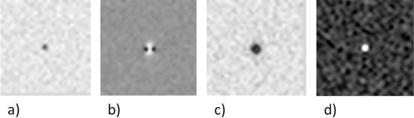
Appearance of a subvoxel (0.5 of a voxel) CMB (Δχ= 3ppm) at 3T on simulated a) magnitude image (a), phase image (b), SWI composite image (n=4) (c) and susceptibility map (SWIM) (d) at TE = 20ms.

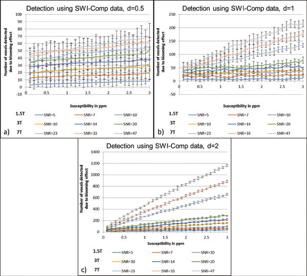
Figure 2.

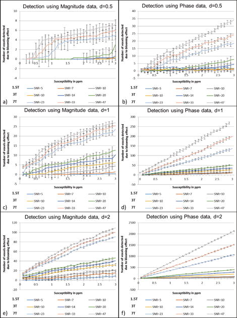
Detection of the CMBs based on the blooming effect on magnitude, phase and SWI composite images from simulations performed at TE = 20ms for 1.5T, 3T and 7T. The CMBs were simulated for three different sizes: diameter of 0.5 of a voxel (a–b), diameter of 1 voxel (c–d) and diameter of 2 voxels as shown in (e–f). The plots represent the number of voxels detected by an intensity threshold of th_mag< 1 – 3 · σ_mag for magnitude images and thφ> 3 · σ_φ, where σ_mag = noise in magnitude images, σ_φ = noise for the phase images. The error represents the Monte Carlo standard deviation, where the error in the mean value was measured from the central voxel of the FOV (where the sphere was positioned) for a number of simulations containing random noise.

The agreement between these formulae and the measured values from the simulations can be seen in Figure 3. The magnitude plot shows non-linearity for lower susceptibility values and becomes linear for susceptibility values after 1ppm. The slope of number of voxels detected versus susceptibility on magnitude images is roughly equal to 5.5d² number/ppm where d is given in pixels. In addition, the effect of voxel aspect ratio was studied and is presented in Figure 4. The increase in slice thickness adversely impacts the phase more than the magnitude image results. When the slice thickness is increased by a factor of 2, the detected number of voxels decreases roughly by a factor of $\sqrt{2}$ for magnitude images and decreases roughly by a factor of 2 on phase images, as seen in Figure 4. Unlike magnitude images, SWI composite images show a linear trend as shown in Figure 5.

Figure 3.

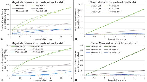
Comparison between measured values and the values derived from our formulae for predicting the number of voxels detected due to blooming effect, for CMBs with diameter = 2 voxels (a–b) and diameter = 1 voxel (c–d). SNR values used for these plots were 47:1 for 7T, 20:1 for 3T and 10:1 for 1.5T simulations.

Figure 4.

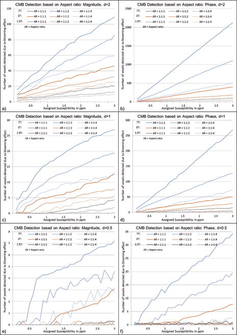
Effects of voxel aspect ratio on CMB detection using magnitude (a,c,e) and phase (b,d,f) images for CMB with a diameter of 2 voxels (a–b), 1 voxel (c–d) and 0.5 voxel (e–f). Simulations were performed at TE = 20ms for 1.5T, 3T and 7T. In these simulations, the highest SNR value is selected for each field strength: 47:1 for 7T, 20:1 for 3T and 10:1 for 1.5T. The CMB size in the simulations was kept constant at a given diameter, while the aspect ratio was varied as 1:1:1, 1:1:2 and 1:1:4 in order to study the detection limits.

Figure 5.

Detection limits on SWI composite images for 2 voxels (a), 1 voxel (b) and 0.5 voxel (c). The plots represent the number of voxels detected by an intensity threshold of th_mag< 1 – 3 · σ_mag for the SWI composite images, where σ_mag = noise in magnitude images. The error represents the Monte Carlo standard deviation, where the error in the mean value was measured from the central voxel of the FOV (where the sphere was positioned) for a number of simulations containing random noise.

The lower echo times tend to be more accurate in measuring mean susceptibility than the higher echo times. On the other hand, the Monte Carlo standard deviation of the mean measured value is higher at short TEs. This is further elaborated by simulations for CMBs with 0.25, 0.5, 1, and 2 voxels in diameter in Figure 6. Although the effective susceptibility is smaller than the actual value, the effective moment turns out to be in agreement with the actual magnetic moment of the object; and almost constant for each case, as shown in Figures 6e and 6f.

Figure 6.

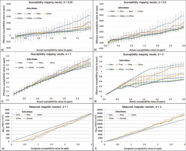
Susceptibility mapping results for CMBs with diameters: 0.25 voxel (a), 0.5 voxel (b), 1 voxel (c) and 2 voxels (d). The effective susceptibility is measured at various TEs: 5ms, 7ms, 9ms, 11ms, 13ms, 15ms and 17ms at 3T when the assigned susceptibility value is varied from 0.1ppm to 3ppm. The standard deviation in the mean susceptibility decreases as TE increases, while the bias relative to the true value increases. However, the magnetic moment is almost independent of echo time for 1 voxel sized CMB (a) and 2 voxels sized CMB (b). [Magnetic moment, μαΔχ_eff · vol, where vol represents effective volume of the object caused by the signal loss.]

Figures 6 and 7 demonstrate the effective mean susceptibility values acquired using SWIM. The effective susceptibility (Δχ_eff) as a function of CMB diameter has volume dependence and is given by:

$$\mathrm{\Delta }{\chi }_{\mathit{\text{eff}}}=0.09\cdot \mathrm{\Delta }\chi \cdot d^3(\text{for}\text{CMB}\text{diameter}\text{up}\text{to}2\text{voxels})$$ [3]

Figure 7.

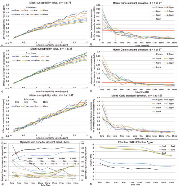
Mean susceptibility values and Monte Carlo standard deviation for the mean susceptibility values at different TEs, when the assigned susceptibility values are varied from 0.1ppm to 3ppm, at 7T at 47:1 (a–b), 3T at 20:1 (c–d) and 1.5T at 10:1 (e–f), respectively. The optimum TE is measured based on the accuracy of the effective susceptibility value and the extent of the Monte Carlo standard deviation. The error reduces considerably at short TEs as the TE increases. The optimal TE value for CMB quantification, at an SNR of 20:1 for susceptibility maps for 1 voxel object with 1ppm susceptibility (which is ±50ppb), is 3ms at 7T, 7ms at 3T and 14ms at 1.5T for CMB diameter = 1voxel, where the error becomes relatively constant. This was studied further by finding the optimal echo time for objects of size more than a voxel (diameter = 1, 2, 4, 6 and 8 voxels), assuming Δχ = 0.5ppm for 3T with SNR_mag = 20:1. The plot in g) shows the balance between σ and ε_r to determine the optimal TE, where σ is the Monte Carlo standard deviation and ε_r is the relative error between the effective susceptibility and the actual value (0.5ppm). The effective SNR for different sized objects based on the effective susceptibility and noise level (σ) is plotted in h).

From this equation, we can say that the measured 1ppm for a CMB with an original diameter of 0.5 voxels suggests that the actual susceptibility can be as high as 89 ppm. The error in measured effective susceptibility is calculated using a Monte Carlo approach. Figure 7 highlights this error and the mean effective susceptibility at various TEs for different field strengths and SNRs, in order to determine the optimum TE for quantification. Although, in theory, one would only need a single plot showing the effect of the ΔχB₀TE product at a given SNR, Figure 7a–f show different plots for different field strengths with a realistic SNR associated with each case for a more accurate error analysis. Hence, apart from the different SNRs, the plots for 1.5T (Figure 7e) and 3T (Figure 7c) are equivalent to a portion of the plot on 7T (Figure 7a) at low and very low susceptibilities. The Monte Carlo error of susceptibility appears more prominent for low echoes and decreases as TE increases. However, it is interesting to note that in Figure 7a, the plots at higher TEs show a more prominent bias in effective susceptibility than at lower TEs. From the plots in Figure 7, for a CMB with a diameter of 1 voxel, a susceptibility of 1ppm and with an SNR of 20:1, we observe that the optimal TE value for CMB quantification would be 3ms at 7T, 7ms at 3T and 14ms at 1.5T where the error becomes less than ±50ppb (5%) representing an SNR of 20:1 (Figure 7). Figures 7g and 7h show that lower TEs are best to produce the more accurate estimates of susceptibility as the object size increases. Prediction of the number of voxels detected and quantified susceptibility were validated using an iron-chitosan phantom study (See Appendix).

DISCUSSION AND CONCLUSIONS

This study was undertaken to provide a comprehensive evaluation of detection sensitivity and quantification of CMBs based on the blooming effect and susceptibility as a function of CMB size relative to the resolution, the product of field strength and echo time, as well as SNR. Multi-voxel CMBs are relatively easy to detect, but sub-voxel bleeds are also particularly important for diseases like cerebral amyloid angiopathy where iron deposits on the order of the size of arterioles (or 50μm) occur.

As the phase signal is linearly proportional to the echo time, longer echo times are essential for detecting phase and magnitude effects for smaller CMBs. Although the signal loss at high TEs is advantageous from the detection standpoint, the size of the CMB will be overestimated due to signal loss (7,8). For this study, we have selected an echo time of 20ms for detection. The trend for magnitude results is non-linear for smaller TEs. This may be due to the difference in the intensities of the regions inside (core) and outside (peri-lesional) the CMBs at increasing TEs, where the perilesional intensity is governed by the T₂* of white matter in our simulations. From our plot of SNR 47:1 for 7T with TE = 20ms, for an object with diameter d not bigger than 1 voxel, we can roughly say that the object is detectable as long as: Δχ > 2.5/(d²) in ppm for magnitude and Δχ > 1.25/(d³) in ppm for phase. Another factor is coil sensitivity that affects local SNR variation across the FOV. In this work, we have included three different SNRs for isotropic resolution, at each field strength. Hence, this concern can be addressed by Figure 2: detection of CMBs at a constant isotropic resolution, where the different SNR values may represent the SNR variations across an image, due to coil sensitivities.

For quantifying the CMBs, the Monte Carlo error was considered to determine the optimal echo time. The lower echo times tend to be more accurate with reduced bias. This bias is caused by the increase in effective size of the object at higher TEs (with a fixed Δχ assigned to the CMB), hence underestimating the susceptibility. This effect is identical to that in Figure 2 where the number of voxels represents the detected blooming effect: as the susceptibility value increases (with a fixed TE for all simulations), the number of voxels losing signal on magnitude images also increases. On the other hand, the Monte Carlo standard deviation of the mean value is higher at short TEs. This shows that the susceptibility reconstruction is more stable in reproducing the results at higher TEs than at shorter TEs. It is also important to note that, using a very long TE would lead to signal loss at the air-tissue interfaces which would obscure the presence of CMBs (23,24). We propose that a dual/multi echo sequence may be used; with one of the echoes being 7ms (for quantification) and another that is a longer echo time (~20ms, for detection).

The predictions for number of voxels detected and the susceptibility measurements made by the simulations in this manuscript are validated using an in vitro phantom with different sizes of iron-chitosan microspheres. The results of the real data match with the simulations and this study is further described in the Appendix. In Figures 6e and 6f, we see that the effective magnetic moment matches with the actual magnetic moment (diameter = 1 and 2 voxel(s) and susceptibility from 0.1 to 3ppm). This is because the magnetic moment is proportional to the product of the effective volume and effective susceptibility and this effective magnetic moment remains almost constant for each echo time. In order to determine the correct volume of the object, the echo time needs to be chosen short enough such that the phase dispersion across the edge voxels is less than π/2 (to retain 90% of the signal) (7,25).

Furthermore, we can estimate the iron content inside the CMB by quantifying the susceptibility using SWIM. The correlation between susceptibility measured by MRI and total iron (C_Fe, measured in μg/ml) by ICPMS for ferritin phantoms is given by: Δχ = 1.1C_Fe − 32.36 (26). Using Eq. [3] for smaller objects, we can derive the total iron content represented by the effective susceptibility:

$$C_{Fe}=\frac{10\cdot \mathrm{\Delta }{\chi }_{\mathit{\text{eff}}}}{d^3}+29.41$$ [4]

In conclusion, SWI can be used to detect iron changes, to find the CMBs and to quantify the iron content. We provide a direct, formulaic approach to estimate the underlying size of the CMB based on the number of radiologically detected voxels, the estimated iron content (using susceptibility mapping) and acquisition parameters. This systematic investigation is anticipated to: improve the interpretation of the radiologically detected CMBs in relation to the underlying degree of the pathology (spatial extent and amount of blood product) and the status of the microbleed (e.g., old or expanding microbleed) and enable the optimal choice of SWI acquisition scheme for the most sensitive detection of pathology.

APPENDIX

Iron-Chitosan phantom study

To validate the predictions described in this manuscript, a phantom consisting of small iron microspheres embedded in agarose gel was used following the procedures in McAuley G et al (2010) (27). The phantom contains microspheres consisting of a chitosan-ferric oxyhydroxide composite at a concentration of approximately 1032μg Fe/g gel (measured analytically), which serves as a mimic for hemosiderin (Figure 8a). The body of the phantom consists of 1.8% (w/v) agarose, 140mM NaCl, 0.5mM NiS04, and 6g/L diazolidinyl urea (preservative). Using the correlation between the concentration of iron and the measured susceptibility of 1.1ppb ≈ 1μg of Fe/ml, we expect the effective susceptibility of the microspheres to be ~1ppm (23).

Figure 8.

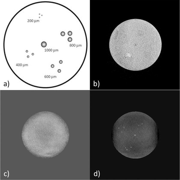
a) Illustration of the in vitro phantom. The phantom consists of iron-chitosan microspheres of diameters: 1000, 800, 600, 400 and 200 μm. b) Original magnitude image, c) SHARP processed phase and d) susceptibility map. The example shown here was acquired with the voxel resolution = (0.5mm)³ isotropic and TE = 20ms.

Image acquisition and processing

The phantom was scanned with two different imaging resolutions of 0.5mm and 1mm isotropic voxel. The imaging parameters were: TE1/TE2/TE3/TE4 = 7/14/20/26ms, FA = 20, TR = 31ms and BW = 260Hz/pixel. The phase images were processed using SHARP to remove any unwanted background field effects. For in vivo data, there is a spatially-variable phase offset term (φ_o) present, along with the TE dependent phase, which will affect the accuracy of the susceptibility reconstruction (10,19,20). Here, φ_o can be calculated using the phase data acquired at TEs = 7ms and 14ms through complex division. A 3 by 3 median filter was applied to reduce the noise. Then, φ_o was removed from the original phase images. The iterative truncated k-space method was applied to generate susceptibility maps from the resultant phase images.

Results

The magnitude images for the 0.5mm isotropic resolution had SNRs of: 12:1, 11:1 and 10:1 for TEs: 7ms, 14ms and 20ms, respectively. The original magnitude and phase, processed phase and susceptibility maps are shown in Figure 8. In order to validate the predictions of the analytical modeling and simulations, the quantified susceptibility values from the in vitro phantom data were compared with simulated results as shown in Table 1. The in vitro results agree with our predictions generated using the analytical model of the spherical CMB.

Table 1.

a) Detected number of voxels on magnitude, processed phase and SWI images of the in vitro iron-chitosan microsphere (μsphere) phantom and b) measured susceptibility (in ppb) from in vitro phantom data acquired at 3T are compared with the predictions shown in Figures 2, 5 and 6. The SNR of magnitude images were 12:1, 11:1 and 10:1 for TEs: 7ms, 14ms and 20ms, respectively.

At TE = 20ms, SNR = 10:1	Diameter = 2		Diameter = 1			Diameter = 0.5
	Number of voxels predicted	In vitro 0.5mm3 (1000μm μsphere)	Number of voxels predicted	In vitro 0.5mm3 (400μm μspheres)	In vitro 1mm3 (1000μm μsphere)	Number of voxels predicted	In vitro 0.5mm3 (200μm μspheres)	In vitro 1mm3 (400μm μspheres)
Magnitude	15	20	2	7	3	0	0	0
Phase	65	58	10	8	9	1	1	1
SWI	46	46	27	17	21	23	10	2
a)

TE (in ms)	Diameter = 2		Diameter = 1			Diameter = 0.5
	Δχ from simulation	In vitro 0.5mm3 (1000μm μsphere)	Δχ from simulation	In vitro 0.5mm3 (400μm μspheres)	In vitro 1mm3 (1000μm μsphere)	Δχ from simulation	In vitro 0.5mm3 (200μm μspheres)	In vitro 1mm3 (400μm μspheres)
7	658	667	322	300	311	15	18	24
14	436	580	280	287	285	11	22	30
20	417	406	283	266	190	8	9	16
b)

Discussion

The iron-chitosan phantom confirms our predictions for the detection and quantification of CMBs on MR images. Following considerations apply while interpreting the results from the phantom.

Since the chitosan ferric oxyhydroxide microspheres were manually embedded in the agarose, it is likely that all 13 microspheres were not embedded in the exact same plane and may be offset by a few microns in the vertical axis. This offset may have contributed to partial volume effect and thus marginal errors in the susceptibility estimate. The analytical measurement of iron content, using the inductively coupled plasma atomic emission spectroscopy (ICP-AES), was performed on the chitosan ferric oxyhydroxide solution from which the microspheres were derived and not from the embedded microspheres. Also, the predictions are generated from the phase images without any source of unwanted background field to remove. The phantom data, however, was processed with the SHARP method. The error caused by using this background removal method will be minimal as the method works on the principle of treating the unwanted field as harmonic component fulfilling the Laplace condition and, hence, removing only the background field from the phase data. Even with the consideration of the above issues, the phantom results were consistent with the simulations.

References

- 1.Shoamanesh A, Kwok CS, Benavente O. Cerebral microbleeds: histopathological correlation of neuroimaging. Cerebrovasc Dis Basel Switz. 2011;32(6):528–34. doi: 10.1159/000331466. [DOI] [PubMed] [Google Scholar]
- 2.Fazekas F, Kleinert R, Roob G, Kleinert G, Kapeller P, Schmidt R, Hartung HP. Histopathologic Analysis of Foci of Signal Loss on Gradient-Echo T2*-Weighted MR Images in Patients with Spontaneous Intracerebral Hemorrhage: Evidence of Microangiopathy-Related Microbleeds. Am J Neuroradiol. 1999 Apr 1;20(4):637–42. [PMC free article] [PubMed] [Google Scholar]
- 3.Greenberg SM, Vernooij MW, Cordonnier C, Viswanathan A, Al-Shahi Salman R, Warach S, Launer LJ, Van Buchem MA, Breteler MM. Cerebral microbleeds: a guide to detection and interpretation. Lancet Neurol. 2009 Feb;8(2):165–74. doi: 10.1016/S1474-4422(09)70013-4. [DOI] [PMC free article] [PubMed] [Google Scholar]
- 4.Park J-H, Park S-W, Kang S-H, Nam T-K, Min B-K, Hwang S-N. Detection of Traumatic Cerebral Microbleeds by Susceptibility-Weighted Image of MRI. J Korean Neurosurg Soc. 2009 Oct;46(4):365–9. doi: 10.3340/jkns.2009.46.4.365. [DOI] [PMC free article] [PubMed] [Google Scholar]
- 5.Kidwell CS, Chalela JA, Saver JL, Starkman S, Hill MD, Demchuk AM, Butman JA, Patronas N, Alger JR, Latour LL, Luby ML, Baird AE, Leary MC, Tremwel M, Ovbiagele B, Fredieu A, Suzuki S, Villablanca JP, Davis S, Dunn B, Todd JW, Ezzeddine MA, Haymore J, Lynch JK, Davis L, Warach S. Comparison of MRI and CT for detection of acute intracerebral hemorrhage. JAMA. 2004 Oct 20;292(15):1823–30. doi: 10.1001/jama.292.15.1823. [DOI] [PubMed] [Google Scholar]
- 6.Mittal S, Wu Z, Neelavalli J, Haacke EM. Susceptibility-Weighted Imaging: Technical Aspects and Clinical Applications, Part 2. Am J Neuroradiol. 2009 Feb 1;30(2):232–52. doi: 10.3174/ajnr.A1461. [DOI] [PMC free article] [PubMed] [Google Scholar]
- 7.Haacke EM, Brown RW, Thompson MR, Venkatesan R. Magnetic Resonance Imaging: Physical Principles and Sequence Design. 2nd. Wiley-Liss; 2014. [Google Scholar]
- 8.Haacke EM, Mittal S, Wu Z, Neelavalli J, Cheng Y-CN. Susceptibility-weighted imaging: technical aspects and clinical applications, part 1. Am J Neuroradiol. 2009 Jan;30(1):19–30. doi: 10.3174/ajnr.A1400. [DOI] [PMC free article] [PubMed] [Google Scholar]
- 9.Haacke EM, Xu Y, Cheng Y-CN, Reichenbach JR. Susceptibility weighted imaging (SWI) Magn Reson Med. 2004 Sep;52(3):612–8. doi: 10.1002/mrm.20198. [DOI] [PubMed] [Google Scholar]
- 10.Haacke EM, Tang J, Neelavalli J, Cheng YCN. Susceptibility mapping as a means to visualize veins and quantify oxygen saturation. 2010 Sep;32(3):663–76. doi: 10.1002/jmri.22276. [DOI] [PMC free article] [PubMed] [Google Scholar]
- 11.Tang J, Liu S, Neelavalli J, Cheng YCN, Buch S, Haacke EM. Improving susceptibility mapping using a threshold-based K-space/image domain iterative reconstruction approach. Magn Reson Med. 2013 May;69(5):1396–407. doi: 10.1002/mrm.24384. [DOI] [PMC free article] [PubMed] [Google Scholar]
- 12.de Rochefort L, Brown R, Prince MR, Wang Y. Quantitative MR susceptibility mapping using piece-wise constant regularized inversion of the magnetic field. Magn Reson Med. 2008;60(4):1003–9. doi: 10.1002/mrm.21710. [DOI] [PubMed] [Google Scholar]
- 13.Shmueli K, de Zwart JA, van Gelderen P, Li T-Q, Dodd SJ, Duyn JH. Magnetic susceptibility mapping of brain tissue in vivo using MRI phase data. Magn Reson Med. 2009 Dec;62(6):1510–22. doi: 10.1002/mrm.22135. [DOI] [PMC free article] [PubMed] [Google Scholar]
- 14.Nandigam RNK, Viswanathan A, Delgado P, Skehan ME, Smith EE, Rosand J, Greenberg SM, Dickerson BC. MR Imaging Detection of Cerebral Microbleeds: Effect of Susceptibility-Weighted Imaging, Section Thickness, and Field Strength. Am J Neuroradiol. 2009 Feb 1;30(2):338–43. doi: 10.3174/ajnr.A1355. [DOI] [PMC free article] [PubMed] [Google Scholar]
- 15.Conijn MMA, Hoogduin JM, van der Graaf Y, Hendrikse J, Luijten PR, Geerlings MI. Microbleeds, lacunar infarcts, white matter lesions and cerebrovascular reactivity – a 7 T study. NeuroImage. 2012 Jan 16;59(2):950–6. doi: 10.1016/j.neuroimage.2011.08.059. [DOI] [PubMed] [Google Scholar]
- 16.Barnes SRS, Haacke EM, Ayaz M, Boikov AS, Kirsch W, Kido D. Semi-Automated Detection of Cerebral Microbleeds in Magnetic Resonance Images. Magn Reson Imaging. 2011 Jul;29(6):844–52. doi: 10.1016/j.mri.2011.02.028. [DOI] [PMC free article] [PubMed] [Google Scholar]
- 17.Cheng A-L, Batool S, McCreary CR, Lauzon ML, Frayne R, Goyal M, Smith EE. Susceptibility-Weighted Imaging is More Reliable Than T2*-Weighted Gradient-Recalled Echo MRI for Detecting Microbleeds. Stroke. 2013 Oct 1;44(10):2782–6. doi: 10.1161/STROKEAHA.113.002267. [DOI] [PubMed] [Google Scholar]
- 18.Brundel M, Heringa SM, de Bresser J, Koek HL, Zwanenburg JJM, Jaap Kappelle L, Luijten PR, Biessels GJ. High prevalence of cerebral microbleeds at 7Tesla MRI in patients with early Alzheimer’s disease. J Alzheimers Dis. 2012;31(2):259–63. doi: 10.3233/JAD-2012-120364. [DOI] [PubMed] [Google Scholar]
- 19.Viswanathan A, Chabriat H. Cerebral Microhemorrhage. Stroke. 2006 Feb 1;37(2):550–5. doi: 10.1161/01.STR.0000199847.96188.12. [DOI] [PubMed] [Google Scholar]
- 20.Cordonnier C, Al-Shahi Salman R, Wardlaw J. Spontaneous brain microbleeds: systematic review, subgroup analyses and standards for study design and reporting. Brain J Neurol. 2007 Aug;130(Pt 8):1988–2003. doi: 10.1093/brain/awl387. [DOI] [PubMed] [Google Scholar]
- 21.Kuijf HJ, de Bresser J, Geerlings MI, Conijn MMA, Viergever MA, Biessels GJ, Vincken KL. Efficient detection of cerebral microbleeds on 7.0 T MR images using the radial symmetry transform. NeuroImage. 2012 Feb 1;59(3):2266–73. doi: 10.1016/j.neuroimage.2011.09.061. [DOI] [PubMed] [Google Scholar]
- 22.Cheng Y-CN, Neelavalli J, Haacke EM. Limitations of calculating field distributions and magnetic susceptibilities in MRI using a Fourier based method. Phys Med Biol. 2009 Mar 7;54(5):1169–89. doi: 10.1088/0031-9155/54/5/005. [DOI] [PMC free article] [PubMed] [Google Scholar]
- 23.Neelavalli J, Cheng Y-CN, Jiang J, Haacke EM. Removing background phase variations in susceptibility-weighted imaging using a fast, forward-field calculation. J Magn Reson Imaging. 2009 Apr;29(4):937–48. doi: 10.1002/jmri.21693. [DOI] [PMC free article] [PubMed] [Google Scholar]
- 24.Buch S, Liu S, Ye Y, Cheng Y-CN, Neelavalli J, Haacke EM. Susceptibility mapping of air, bone, and calcium in the head. Magn Reson Med. 2015 Jun;73(6):2185–94. doi: 10.1002/mrm.25350. [DOI] [PubMed] [Google Scholar]
- 25.Liu S, Neelavalli J, Cheng Y-CN, Tang J, Mark Haacke E. Quantitative susceptibility mapping of small objects using volume constraints. Magn Reson Med. 2013 Mar 1;69(3):716–23. doi: 10.1002/mrm.24305. [DOI] [PMC free article] [PubMed] [Google Scholar]
- 26.Zheng W, Nichol H, Liu S, Cheng Y-CN, Haacke EM. Measuring iron in the brain using quantitative susceptibility mapping and X-ray fluorescence imaging. NeuroImage. 2013 Sep;78:68–74. doi: 10.1016/j.neuroimage.2013.04.022. [DOI] [PMC free article] [PubMed] [Google Scholar]
- 27.McAuley G, Schrag M, Sipos P, Sun S-W, Obenaus A, Neelavalli J, Haacke EM, Holshouser B, Madácsi R, Kirsch W. Quantification of punctate iron sources using magnetic resonance phase. Magn Reson Med. 2010 Jan;63(1):106–15. doi: 10.1002/mrm.22185. [DOI] [PubMed] [Google Scholar]