

Abstract
Theoretical properties of a multi-scale opening (MSO) algorithm for two conjoined fuzzy objects are established, and its extension to separating two conjoined fuzzy objects with different intensity properties is introduced. Also, its applications to artery/vein (A/V) separation in pulmonary CT imaging and carotid vessel segmentation in CT angiograms (CTAs) of patients with intracranial aneurysms are presented. The new algorithm accounts for distinct intensity properties of individual conjoined objects by combining fuzzy distance transform (FDT), a morphologic feature, with fuzzy connectivity, a topologic feature. The algorithm iteratively opens the two conjoined objects starting at large scales and progressing toward finer scales. Results of application of the method in separating arteries and veins in a physical cast phantom of a pig lung are presented. Accuracy of the algorithm is quantitatively evaluated in terms of sensitivity and specificity on patients' CTA data sets and its performance is compared with existing methods. Reproducibility of the algorithm is examined in terms of volumetric agreement between two users' carotid vessel segmentation results. Experimental results using this algorithm on patients' CTA data demonstrate a high average accuracy of 96.3% with 95.1% sensitivity and 97.5% specificity and a high reproducibility of 94.2% average agreement between segmentation results from two mutually independent users. Approximately, twenty-five to thirty-five user-specified seeds/separators are needed for each CTA data through a custom designed graphical interface requiring an average of thirty minutes to complete carotid vascular segmentation in a patient's CTA data set.
Index Terms: Fuzzy connectivity, fuzzy distance transform, morphology, multi-scale opening, CTA, carotid vasculature, pulmonary vasculature
I. Introduction
Multi-Layered extraction of knowledge embedded in two- and higher-dimensional images has remained a front-line research aim over several decades [1]–[8]. Often, segmentation of one or multiple objects in an image presents a major challenge in many such applications. Despite paramount research efforts on image segmentation over the last several decades [9]–[15], there is no universally acceptable segmentation method and, often, we face new segmentation tasks that may not be efficiently solved within the conventional framework. Here, we address one such segmentation task where the challenge lies in separating two fuzzy objects fused at various unknown locations and scales [16]–[18]. The background and the area of applications along with literature survey, evolution of the current algorithm and novel contributions in this paper are discussed in the following.
Background and the Area of Applications
The method presented in this paper is described in the context of two important medical imaging applications—(1) pulmonary artery/vein (A/V) separation in chest CT imaging and (2) segmentation of carotid vasculature in CT angiograms (CTAs) of patients with intracranial aneurysms. Separating pulmonary A/V trees via CT imaging is a crucial step in the quantification of vascular geometry for the purpose of determining pulmonary hypertension, pulmonary emboli, emphasyma and more. The couplings or fusions between A/V trees are tight and complex attributed with arbitrary and multi-scale geometry, especially at branching locations. Limited signal-to-noise ratio (SNR), relatively low spatial resolution and subject-specific structural variations of vascular trees further complicate the task. Previous works from our group on multi-scale opening (MSO) algorithm [17], [19] have been applied successfully for separation of A/V trees in non-contrast CT imaging. Here, we extend the application where arteries and veins are assigned separate CT image contrasts.
In regards to the other application, intracranial aneurysms are acquired lesions (5-10% of the population), a fraction of which rupture leading to subarachnoid hemorrhage with devastating clinical consequences. From an imaging perspective, intracranial aneurysms are abnormal outpouchings in the cerebral vasculature. Such aneurysms occur predominantly in or near the Circle of Willis—a circular configuration of arteries in the base of the brain. They are usually anywhere from a few millimeters to several centimeters [20], [21] in diameter. Treatments include microsurgical clipping, endovascular insertion of coils into the aneurysm and/or deployment of stents for diverting blood flow. However, such treatments are themselves associated with some mortality and morbidity. Therefore, it is prudent to avoid surgery if the risk of rupture is deemed minimal, and the clinical management of these lesions would benefit from a better understanding of factors associated with rupture risk. In this context, studies on morphological characteristics, hemodynamics and aneurysm tissue mechanics become valuable. Key to such computational risk-assessment approaches is the ability of accurate and rapid segmentation of the vasculature with the aneurysm in the brain. Further, cerebral vessel segmentation will also aid in surgical planning and serial follow-up of patients [22]. In the arena of both clinical research as well as patient care, CTAs are popularly used to evaluate intracranial aneurysms. In CTA, bone picks higher intensities and soft tissue, fat, and skin appear with lower intensities while the intensity range for the vascular tree falls in between [23]. The major challenge in segmenting the carotid vasculature is the coupling between vessels and bone structures at unknown and variable scales, especially, at the vicinity of sinus and nasal regions. These challenges are further enhanced by – (1) shared intensity band between the two objects at limited SNR and spatial resolution and (2) unknown complex geometry of thin bones near carotid sinus. Depending upon the applied contrast protocol [24], [25], intensities of either the artery or both artery and vein trees are enhanced during the patients' carotid CTA.
Literature Survey
Several algorithms [26]–[30] are available in literature on segmentation of cerebral aneurysms. Steinman and colleagues reported on a semi-automatic algorithms for 3D reconstruction of giant aneurysms on the posterior communicating artery using a discrete dynamic contouring approach [29]. Subsequently, Cebral and colleagues [26] presented a 3D reconstruction algorithm for cerebral aneurysms using level sets and deformable models. Frangi and his colleagues have used a region-based implicit surface modeling approach [27], [28], [30] to accomplish the task. However, these algorithms primarily focus on segmenting a cerebral aneurysm and a small part of the attached vessel rather than the entire cerebral vessel tree. Reconstruction of the complete cerebral vasculature permits hemodynamic analyses with a greater contextual information and, therefore, enhancing the quality of analytic results. Also, it is difficult to segment aneurysms when they lie in close proximity to the skull (common in aneurysms at the internal carotid artery) or to neighboring vessels (common in anterior communicating artery aneurysms). These challenges have not been thoroughly addressed in previous studies. Moreover, existing algorithms rely on significant user interaction and, therefore, final results are susceptible of subjectivity errors. However, dependence of these algorithms on user input has not been thoroughly investigated.
Evolution of the Current Algorithm and Novel Contributions in this Paper
In this paper, the fundamental challenges of pulmonary A/V separation and vessel segmentation in CTA are solved using a new MSO algorithm that is capable of separating both intensity-similar as well as intensity-varying conjoined fuzzy objects. The MSO [17] algorithm was originally presented for medical image processing research community and its application to separate two similar-intensity objects were demonstrated. Here, theoretical properties of the MSO algorithm are established and its domain is extended to separate mutually fused fuzzy objects with different intensity properties. We address two important applications of the new algorithm – (1) separation of A/V from CT imaging of a pig lung phantom and (2) separation of carotid vasculature from bones in CTAs of patients with intracranial aneurysms. A short version of the MSO algorithm for separation of two objects sharing different intensity properties that are fused at unknown locations and scales, was presented in a conference paper [31] targeted to biomedical imaging and instrumentation research community. The novel contributions of this paper as compared to our previous works include – (1) a detailed and formal presentation of a modified MSO algorithm, (2) analytic proofs of disjoincy of separated objects and termination of the algorithm in a finite number of steps, (3) new experiments and results on A/V separation with different intensity properties, multi-user reproducibility, accuracy analysis on a larger dataset of patients' CTA, and comparison with existing algorithms. It may be noted that the premise of the MSO algorithm is developed by combining the theories of fuzzy distance transform (FDT) [32], [33], fuzzy connectivity [15], [34], [35], and iterative relative fuzzy connectivity [36]–[38]. Further, it may be emphasized that our algorithm is independent of the contrast protocol used in CT imaging of pulmonary A/V or in CTA.
The theory and properties of multi-scale separation of two conjoined fuzzy objects are established in Section II. Algorithm design for separation of conjoined fuzzy objects with different intensity properties is presented in Section III, while the experimental methods and results are discussed in Section IV. Finally, the conclusion is drawn in Section V.
II. Theory of Multi-Scale Opening for Conjoined Fuzzy Objects
In this section, we describe the MSO algorithm [17], [19] separating two similar-intensity fuzzy objects conjoined at various locations and scales and establish its theoretical properties. Expansion of the domain of application of the algorithm where the fused objects possess different intensity characteristics is discussed in the next section.
A. Basic Definitions and Notations
A three dimensional (3D) cubic grid, or simply a cubic grid, is represented by Ƶ3 | Ƶ is the set of integers. A grid point, often referred to as a point or a voxel, is an element of Ƶ3 and is represented by a triplet of integer coordinates. Standard 26-adjacency [39] is used here, i.e., two voxels p = (x1, x2, x3), q = (y1, y2, y3) ∈ Ƶ3 are adjacent if and only if max1≤i≤3 |xi − yi| ≤ 1, where | · | gives the absolute value. Two adjacent voxels are often referred to as neighbors of each other; the set of 26-neighbors of a voxel p excluding itself is denoted by 𝒩*(p) An object 𝒪 is a fuzzy subset {(p, μ𝒪(p)) | p ∈ Ƶ3}, where μ𝒪 : Ƶ3 → [0, 1] is the membership function. The support Θ(𝒪) of an object 𝒪 is the set of all voxels with non-zero membership, i.e., Θ(𝒪) = {p | p ∈ Ƶ3 and μ𝒪 (p) ≠ 0}; Θ̄(𝒪) = Ƶ3 − Θ(𝒪) is the background. Images are always acquired with a finite field of view. Thus, we will assume that an object has a bounded support.
Let S denote a set of voxels; a path π in S from p ∈ S to q ∈ S is a sequence 〈p = p1, p2, ⋯, pl = q〉 of voxels in S such that every two successive voxels are adjacent. A link is a path 〈p, q〉 of exactly two adjacent voxels. The length of a path π = 〈p1, p2, ⋯, pl〉 in a fuzzy object 𝒪, denoted as Π𝒪(π), is the sum of lengths of all links on the path, i.e.,
| (1) |
where, ‖pi − pi+1‖ is the Euclidean distance between p, q. The fuzzy distance [32], [33] between two voxels p, q ∈ Ƶ3 in an object 𝒪, denoted by ω𝒪(p, q), is the length of one of the shortest paths from p to q, i.e.,
| (2) |
where, 𝒫(p, q) is the set of all paths from p to q. The FDT of an object 𝒪 is an image {(p, Ω𝒪(p)) | p ∈ Ƶ3}, where Ω𝒪 : Ƶ3 → ℛ+ | ℛ+ is the set of positive real numbers including zero, is the fuzzy distance from the background, i.e.,
| (3) |
Here, we use “local scale” of an object voxel as the depth or FDT value at the closest locally-deepest voxel. Specifically, a voxel p ∈ Θ(𝒪) is locally-deepest if ∀q ∈ 𝒩l(p), Ω𝒪(q) ≤ Ω𝒪(p), where 𝒩l(p) is the (2l +1)3 neighborhood of p; here, 𝒩2(p) is used to avoid noisy local maxima. Let Smax ⊂ Θ(𝒪) be the set of all locally-deepest voxels. Local scale of a voxel p, denoted as δ𝒪(p), is the FDT value of the voxel in Smax that is nearest to p; in case of a tie, the voxel with larger FDT value is chosen. FDT value at each voxel p is normalized by dividing it with local scale δ𝒪 (p) to reduce effects of spatial scale variation. Now onward, both “FDT” and Ω𝒪 will refer to “scale-normalized FDT” unless stated otherwise.
Let us comeback to the segmentation task where the challenge is to separate two fuzzy objects 𝒪𝒜 and 𝒪ℬ, which are fused at various unknown locations and scales. This task is solved using a new MSO algorithm in two sequential steps – Step 1: segmentation of the combined region 𝒪𝒜 ∪ 𝒪ℬ from the background, and Step 2: separation of 𝒪𝒜 and 𝒪ℬ. The first step may trivially be achieved using simple thresholding [40], [41] and connectivity analysis [42], [43]. Let 𝒪 be the fuzzy segmentation of the combined region obtained in Step 1. All subsequent analyses will be confined to the support Θ(𝒪) of 𝒪 which will be the “effective image space”; let I : Θ(𝒪) → [Imin, Imax] be image intensity function over Θ(𝒪).
In the second step, the separation task is modeled as an opening algorithm of two fuzzy objects mutually fused at different unknown regions and scales. Often, a simple fuzzy connectivity or edge analysis may not be suitable to separate the two structures. On the other hand, the two objects may frequently be locally separable using a suitable morphological opening operator. The challenges here are – (1) how to determine local size of suitable morphological operators and (2) how to combine the locally separated regions. The MSO algorithm combines fuzzy distance transform (FDT) [32], [33] a morphologic function with a topologic fuzzy connectivity [35], [44]–[46] to iteratively open the two objects starting at large scales and progressing toward finer scales.
B. Optimal Erosion using Morpho-Connectivity
Here, we define the algorithm for the first iteration. The basic idea of this step is to gradually erode the assembly of two fused fuzzy objects until those two objects get mutually disconnected creating two separate objects. It starts with two sets of seed voxels S𝒜 and Sℬ and a set of common separators S𝒮 The initial FDT map Ω𝒜,0 for the first object is computed from 𝒪 except that the voxels in Sℬ ∪ S𝒮 are added to the background; it is worth mentioning that the local scale map δ𝒪, derived from the original assembled object 𝒪, is used for normalization. FDT map Ωℬ,0 for the other object is computed similarly. It is reasonable to assume that the sets S𝒜, Sℬ, and S𝒮 are mutually exclusive.
Fuzzy morpho-connectivity strength of a path π = 〈p1, p2, ⋯, pl〉 in a fuzzy object 𝒪, denoted as Γ𝒪(π), is the minimum FDT value along the path:
| (4) |
Fuzzy morpho-connectivity between two voxels p, q ∈ Ƶ3, denoted as γ𝒪 (p, q), is the strength of the strongest morphological paths between p and q, i.e.,
| (5) |
Definition 1. Optimum erosion of a fuzzy object 𝒜 represented by the set of seed voxels S𝒜 with respect to its co-object ℬ represented by the set of seed voxels Sℬ and a set of common separator S𝒮 is the set of all voxels p such that there exists an erosion scale that disconnects p from ℬ while leaving it connected to 𝒜, i.e.,
| (6) |
where, the fuzzy morpho-connectivity functions γ𝒜,0 and γℬ,0 are defined from the FDT maps Ω𝒜,0 and Ωℬ,0, respectively. The optimum erosion Rℬ,0 of the object ℬ is defined similarly.
Proposition 1. For any fuzzy object 𝒪 in Ƶ3, for any two mutually exclusive sets of seeds S𝒜 and Sℬ, representing two different objects, and a set of common separator S𝒮 disjoint to both S𝒜 and Sℬ, the separated regions R𝒜,0, Rℬ,0, after optimum erosion, are always disjoint, i.e., R𝒜,0 ∩ Rℬ,0 = ∅.
Proof. To prove this proposition by contradiction, first, let us assume that the proposition is not true, i.e., R𝒜,0 ∩ Rℬ,0 ≠ ∅. Let us consider a voxel p ∈ R𝒜,0∩Rℬ,0. Following Equation 6 and our assumption that the voxel p belongs to R𝒜,0, we get maxa∈S𝒜 γ𝒜,0(a, p) > maxb∈Sℬ γℬ,0 (b, p). But since the voxel p also belongs to Rℬ,0 according to our assumption, following the same equation, we get maxb∈Sℬ γℬ,0 (b, p) > maxa∈S𝒜 γ𝒜,0(a, p). Hence contradiction.
C. Constrained Dilation
The two optimally eroded regions R𝒜,0 and Rℬ,0 (Fig. 1(a)) separates the two target objects using morpho-connectivity. However, each of these two separated regions captures only an eroded version of the target objects over respective local regions and dilation is needed to further improve the delineation results (Fig. 1(b)). Also, the annular left-over from optimal erosion (Fig. 1(a)) wrongly permits path leakages from one separated region into the other. It is crucial to block such leakages in order to proceed with the separation process to the next finer scale. Both objectives are fulfilled by local dilation of the two separated objects and we refer to it as a “constrained dilation” to emphasize that the process must preserve separate identities of the two objects (Fig. 1(b)). Constrained dilation is applied over a “morphological neighborhood” to ensure that the dilation is locally confined. The purpose of morphological neighborhood is to define a morphological locality that matches with the scale and geometry of the local structure.
Fig. 1.

A schematic illustration of the results of different steps in the MSO algorithm—(a) optimal erosion, (b) constrained dilation, and (c) iterative progression to the next iteration.
Definition 2. Morphological neighborhood of a set of voxels X in an object 𝒪, denoted by N𝒪(X), is a set of all voxels p ∈ Θ(𝒪) such that ∃q ∈ X for which ω𝒪(p, q) < Ω𝒪(q) and p is connected to q by a path π = 〈p = p1, p2, ⋯, pl = q〉 of monotonically increasing FDT values.
In Definition 2, the original FDT map without scale normalization is used as morphological neighborhood should capture original un-normalized scale and geometry of the local structure.
Definition 3. Constrained dilation of R𝒜,0 with respect to its co-object Rℬ,0 within the fuzzy object 𝒪, denoted as M𝒜,0, is the set of all voxels p ∈ N𝒪 (R𝒜,0), which are strictly closer to R𝒜,0 than Rℬ,0 (Fig. 1(b)), i.e.,
| (7) |
where, the fuzzy distance function ω𝒪 is defined over the fuzzy object 𝒪 in Ƶ3. The region Mℬ,0 is defined similarly.
It may be noted that, gaps between the separated regions visible in Fig. 1(a) are filled in Fig. 1(b) after constrained dilation, and thus, undesired paths running through those gaps are blocked enabling separation at the next finer scale. The two steps of optimal erosion and constrained dilation lead to an “optimal opening” operation preparing the ground for separation at next finer scales.
Proposition 2. For any fuzzy object 𝒪 in Ƶ3, for any two mutually exclusive sets of seeds S𝒜 and Sℬ, representing two different objects, and a set of common separator S𝒮 disjoint to both S𝒜 and Sℬ, the constrained dilations M𝒜,0, Mℬ,0 are always disjoint, i.e., M𝒜,0 ∩ Mℬ,0 = ∅.
Proof. To prove this proposition by contradiction first let us assume that the proposition is not true, i.e., M𝒜,0 ∩ Mℬ,0 ≠ ∅. Let us consider a voxel p in M𝒜,0 ∩ Mℬ,0. Following the assumption that p ∈ M𝒜,0 and Definition 3, we get mina∈R𝒜,0 ω𝒪(a, p) < minb∈Rℬ,0 ω𝒪(b, p). Therefore p is strictly closer to R𝒜, 0. But, since p also belongs to Mℬ,0, following Definition 3, we get minb∈Rℬ,0 ω𝒪(b, p) < mina∈R𝒜,0 ω𝒪(a, p), making p strictly closer to Rℬ,0 as well. Therefore the voxel p cannot be strictly closer to both R𝒜,0 and Rℬ,0 simultaneously. Hence the contradiction.
Corollary 1. For any fuzzy object 𝒪 in Ƶ3, for any two mutually exclusive sets of seeds S𝒜 and Sℬ, representing two different objects, and a set of common separator S𝒮 disjoint to both S𝒜 and Sℬ, the constrained dilations M𝒜,0 and Mℬ,0 include the optimum erosions R𝒜,0 and Rℬ,0, respectively, i.e., R𝒜,0 ⊂ M𝒜,0 and Rℬ,0 ⊂ Mℬ,0.
D. Iterative Progression to Multi-Scale Opening
The optimal opening algorithm, as described above, separates two target objects at a specific scale and the purpose of the current step is to freeze the boundary of previous separation enabling propagation to the next finer scale. This step operates in a fashion similar to the iterative strategy described in references [36]–[38] for intensity based fuzzy connectivity. For each of the two objects, we set the FDT values to zero over the region currently acquired by its rival object. It puts a hypothetical wall at the boundary of each object separated in the previous iteration stopping paths from one object to run through the territory already acquired by the rival object. Specifically, after each iteration, the FDT image of object 𝒜 is updated as follows:
| (8) |
The FDT map of the other object is updated similarly. The seed voxels S𝒜 and Sℬ for the two objects are replaced by M𝒜,i−1 and Mℬ,i−1 respectively (Fig. 1(c)). With this set-up the algorithm enters into the next iteration and the morphological separations M𝒜,i and Mℬ,i are derived using the Equations 6—8 and Definitions 1—3.
Proposition 3. For any fuzzy object 𝒪 in Ƶ3, for any two mutually exclusive sets of seeds S𝒜 and Sℬ, representing two different objects, and a set of common separator S𝒮 disjoint to both S𝒜 and Sℬ, for any positive integer i, the separation results M𝒜,i, Mℬ,i of the MSO algorithm are always disjoint, i.e., M𝒜,i ∩ Mℬ,i = ∅.
Proof. This proposition will be proved by induction. From Proposition 1, we get R𝒜,0 ∩ Rℬ,0 = ∅ and from Proposition 2 we get M𝒜,0 ∩ Mℬ,0 = ∅. This ensures disjoint separation of the two fuzzy objects after the first iteration of the MSO algorithm. Let us assume that this proposition is true after (i − 1)th iteration, for some i ≥ 1. To complete the proof, we will show that the proposition remains true after the ith iteration. During the ith iteration of multi-scale opening, the following changes take place in the optimum erosion and iterative progression steps as compared to the first iteration: Ω𝒜,0 (or, Ωℬ,0) is replaced by Ω𝒜,i (respectively, Ωℬ,i) in Equation 6 and the set seeds S𝒜 is replaced by M𝒜, i−1, while Sℬ is replaced by Mℬ, i−1. Therefore, following Propositions 1 and 2, the results of optimum erosion and constrained dilation, the output separation of the ith iteration remain disjoint, i.e., M𝒜,0 ∩ Mℬ,0 = ∅.
Proposition 4. For any fuzzy object 𝒪 in Ƶ3, for any two mutually exclusive sets of seeds S𝒜 and Sℬ, representing two different objects, and a set of common separator S𝒮 disjoint to both S𝒜 and Sℬ, for any positive integer i, the separation results M𝒜,i ⊂ M𝒜,i+1.
Proof. Following iterative progression of multi-scale opening, during the (i + 1)th iteration, M𝒜,i is used as the set of seeds for the object 𝒜. Following Definition 3, we get M𝒜,i ⊂ N𝒪 (R𝒜,i); and following Proposition 3, we get M𝒜,i ∩ Mℬ,i = ∅. Therefore, p ∈ M𝒜,i = M𝒜,i − Mℬ,i, ⊂ N𝒪 (R𝒜,i) − Mℬ,i. Thus, following Equation 8, ∀p ∈ M𝒜,i, Ωℬ,i+1(p) = 0. Hence, following Equations 4—6, M𝒜,i ⊂ R𝒜,i+1 ⊂ M𝒜,i+1.
Proposition 5. For any fuzzy object 𝒪 in Ƶ3, for any two mutually exclusive sets of seeds S𝒜 and Sℬ, representing two different objects, and a set of common separator S𝒮 disjoint to both S𝒜 and Sℬ, the MSO algorithm terminates in a finite number of iterations.
Proof. For all voxels, p ∈ Θ̄(𝒪), for any i ≥ 0, the FDT maps Ω𝒜,i(p) = Ωℬ,i(p) = 0. Therefore, following Equations 4—6, R𝒜,i,Rℬ,i ⊂ Θ(𝒪). Following Definition 2, the morphological neighborhoods N𝒪(R𝒜,i), N𝒪(Rℬ,i) ⊂ Θ(𝒪). Therefore, the results of constrained dilation M𝒜,i and Mℬ,i are confined to the finite set Θ(𝒪). Again, following Proposition 4, M𝒜,i and Mℬ,i are monotonically non-contracting. Therefore, after a finitely many iterations, both of these sets converge when the MSO algorithm terminates.
III. Multi-Scale Opening of Conjoined Objects with Different Intensity Characteristics
Previous algorithms [17], [19] of multi-scale opening for two conjoined objects assume that the two objects share a common intensity characteristic. Here a revised formulation of the MSO algorithm is presented where the two conjoined fuzzy objects possess different intensity characteristics with an overlapping shared intensity band. Let us explain the algorithm from the perspective of carotid vessel segmentation in human CTAs; however, similar formulation works for the other application of A/V separation in pig lung phantom CT imaging. First, the segmentation of combined regions for bone and vessels (in the rest of this paper by “vessel” we will refer to the vasculature together with aneurysms, if any) is completed. Subsequently, the MSO algorithm is applied to separate vessels from bone. The first step is achieved in CTA using simple thresholding [40], [41] and connectivity analysis [42], [43]. Let 𝒪 be the fuzzy segmentation of the combined bone and vessels after removing low intensity regions mostly occupied by soft tissue and skin. All subsequent analyses are confined to the support Θ(𝒪) of 𝒪 representing the effective image space; let ICTA : Θ(𝒪) → [Imin, Imax] be CTA image intensity function. Major challenges in our carotid vessel segmentation approach are embedded in the second step, i.e., separation of vasculature from bone which is modeled here as opening two fuzzy objects with different intensity characteristics while sharing a common intensity band and mutually fused at unknown locations and scales.
Let us consider the coupling of two objects illustrated in Fig. 2(a) where a bone-like structure (green) and a vessel (red), with significant intensity overlap (Fig. 2(b)), are fused with each other at unknown locations and scales. Color-coded combined vessel (red channel) and bone (green channel) membership maps on a CTA axial image slice is shown in Fig. 2(c). Let μbone and μvessel denote the bone and vessel membership functions defined as follows:
Fig. 2.

A schematic description of challenges in separating bone and vasculature in CTA. (a) Multi-scale fusion of bone (green) and vessel (red) demands local scale-adaptive opening. (b) Intensity-based membership functions for vessel and bone along with pure and shared intensity bands. (c) Color-coded combined vessel and bone membership maps on an axial image slice in a patient's CTA. Regions indicated in pure green are pure bone; here, no pure vessel region is identified and therefore all other regions fall in the shared space. The figures shown in (a) and (b) were previously published by the authors in an IEEE conference paper [31].
| (9) |
| (10) |
where, Ivessel and Ibone are representative vessel and bone intensities defining the respective transition between pure and shared intensity bands (Fig. 2(b)). Let Pbone ⊂ Θ(𝒪) (or, Pvessel ⊂ Θ(𝒪)) be the set of voxels falling inside the pure intensity band for bones (respectively, vessels). Thus, the set of voxels falling within the shared intensity band is Oshared = Θ(𝒪) − Pbone − Pvessel. A fuzzy representation of the composite object may be obtained by taking the fuzzy union of the two membership functions shown in Equations 9 and 10.
An overall work flow diagram of the MSO algorithm for two fuzzy objects with different intensity properties are is presented in Fig. 3. In the iterative approach of multi-scale opening of two structures, it takes several iterations to grow path-continuity of an object starting from its seed voxels, commonly added in large scale regions, to a peripheral location with fine scale details. This phenomenon of gradual extension of an object within the MSO framework may lead to a challenge in separating peripheral structures in some applications, e.g., separation of vasculature from bone in CTA. Let us consider the following situation – a peripheral voxel, say p, of the vascular object, say 𝒪𝒜, come to the vicinity of pure intensity regions of its rival bone object, say 𝒪ℬ, and gets fused. Due to the iterative nature of multi-scale progression model in the MSO separation algorithm, it takes several iterations for vasculature 𝒪𝒜 to propagate its path continuity from seed voxels (primarily located at central regions) to the peripheral voxel p along the paths in the vascular structure. On the other hand, the path-continuity of 𝒪ℬ reaches to p quicker due to immediate spatial vicinity of p and pure intensity region of 𝒪ℬ which are included as seed voxels. Thus, p may be seized by 𝒪ℬ before a path from a seed voxel of 𝒪𝒜 reaches there in the process of iterative gradual multi-scale progression. This problem is solved by using a one voxel thick prohibited region P around pure intensity regions of both objects. It may be noted that for most applications, since no pure intensity zone is assigned for the lower intensity object, P only surround the brighter intensity object. This allows lower intensity objects to reach peripheral sites through iterations. Finally, the MSO algorithm runs in two sequential phases. During the first phase, the separation is confined to Θ(𝒪) − P and then, in the second phase, the separation is made open to the entire Θ(𝒪).
Fig. 3.

A modular representation of the MSO algorithm.
IV. Experimental Methods and Results
To facilitate the experimental methods, an integrated custom-designed 2-D/3-D graphical user interface was developed in our laboratory allowing simultaneous viewing of 2-D and 3-D geometry of target objects along with current segmentation results using different options for overlay colors. The correspondence of target object geometry in 3-D and three planar views is realized by tagging the 3-D cursor with 2-D planar cursors. Facilities of selecting and editing different seeds and separators are supported within the graphical interface along with various display and overlay-related options.
Results of application of the algorithm to a CT image of a pig lung cast phantom with different CT contrasts for arterial and venous trees are presented in Fig. 4. To generate the pig pulmonary vessel cast phantom, the animal was first exsanguinated. While maintaining ventilation at low positive end-expiratory pressure (PEEP), the pulmonary vasculature was flushed with 1L 2% Dextran solution and pneumonectomy was performed. While keeping the lungs inflated at approximately 22 cm H2O Pawy, a rapid hardening methyl methacrylate compound (Orthodontic Resin, DENTSPLY International, York, PA) was injected into the vasculature to create a cast of the pulmonary arterial and venous trees. The casting compound was mixed with red oil paint for the venous (oxygenated) side and blue oil paint for the arterial (deoxygenated) side of the vascular beds. The arterial side was also contrast-enhanced by the addition of 10 cc of Ethiodol (Savage Laboratories, Melville, NY) to the casting compound (Fig. 4(a)). The vessel cast was scanned on a Siemens Somatom Definition Flash 128 CT scanner using the following protocol − 120 kV, 115 effective mAs, 1-s rotation speed, pitch factor: 1.0, nominal collimation: 16 mm×0.3 mm, image matrix: 512×512 and (0.34 mm)2 in-plane resolution, and 0.75 mm slice thickness.
Fig. 4.
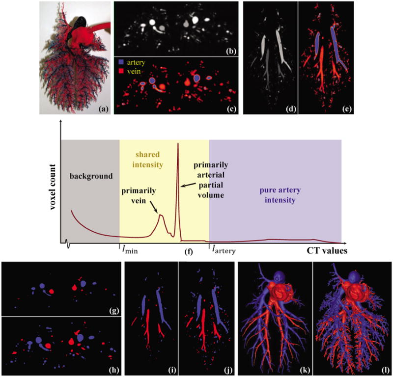
A/V separation on a pulmonary pig vessel cast phantom. (a) A photograph of the phantom. (b) An axial image slice from the phantom CT image with different contrast for A/V trees. (c) CT intensity-based A/V classification showing partial voluming effects as thin red films wrapping around blue arteries. (d,e) Same as (b,c) on a coronal image slice. (f) CT intensity histogram of the phantom where the two CT intensity values Imin and Iartery segments the background and pure artery regions. (g) Optimum thresholding and morphological erosion are applied on (b) to separate the core arteries and veins. (h) A/V separation on (b) using the MSO algorithm. (i,j) Same as (g,h) on the matching coronal image slice of (d,e). (k) 3-D rendering of A/V separation using optimum thresholding morphological erosion. (l) Same as (k) but using the MSO algorithm.
Axial (Fig. 4(b)) and coronal (Fig. 4(d)) image slices from the original CT images of the pig-lung phantom are shown along with the intensity histogram (Fig. 4(f)); in Fig. 4(f), the part of the histogram for the background region is only partially shown. Two CT intensity values Imin and Iartery segmenting the background and pure artery regions were manually selected by three independent users and the mean values were selected as shown in Fig. 4(f). Although, the histogram show a mode of CT values for veins, no intensity values could be selected as pure vein intensity as partially volume artery voxels share those intensity values. Therefore, the intensity range [Imin, Iartery] was used as the shared intensity space. A sharp peak was identified as primarily contributed by partial voluming of arteries; however, this information is not used by the algorithm. The CT intensity-based classification of artery and vein is shown in Fig. 4(c) and Fig. 4(e) where the partial voluming effect appears as a thin red films wrapping around arteries.
A thresholding and morphological erosion was applied to separate the core arteries and veins, and the results are shown in Fig. 4(g, i, k). Such an approach succeeds to capture core arteries and veins but fails to preserve fine details due to partial voluming. The superiority of the new MSO algorithm lies in its ability to trace fine structures of individual objects despite the presence of partial voluming and intensity sharing. The results of A/V separation using the MSO algorithm are shown in Fig. 4(h, j, l) which successfully capture fine details. For this experiment, two seed voxels were used for arteries and another three seed voxels were used for veins using our custom 2D/3D graphical interface.
The overall aim of our experimental plan is to examine the accuracy, reproducibility, and efficiency of the MSO algorithm for separating two fuzzy objects with distinct intensity characteristics but sharing a common intensity band while conjoined at unknown locations and scales. For quantitative evaluation of the accuracy of the algorithm, we used image data from human cerebral CTAs. Inter-user reproducibility of the method was examined using results of bone-removed vessel segmentation in human carotid CTAs obtained by interactive inputs from two mutually-blinded independent users. In the following subsections, we describe detail plans, methods and results for each of these experiments. The efficiency of the algorithm is reported in terms of the number of user specified seed voxels and separators and user interaction time for different experiments. Also, the average computation time for the algorithm is reported.
A. Accuracy
The accuracy of the algorithm on mathematical phantoms with known truths was examined and the results were presented in [31]. Although the phantoms were designed to simulate various geometry of coupling between two objects, it's difficult to simulate the complexity of coupling between two objects present in a true biological environment. Here, we evaluate the accuracy of our algorithm on patients' carotid CTA datasets and compare its performance with existing algorithms.
An axial image slices from a carotid CTA and the intensity-based bone-vessel classification results are shown in Fig. 5(a, b); the CT intensity histogram is presented in Fig. 5(c). It is evident from Fig. 5(b) that carotid vasculature and soft/thin bones appear with similar CT intensities. To evaluate the performance of the algorithm, ten CTA data sets were collected using Siemens Somatom Sensation 16 scanner at 120 kV, rotation time of 0.5 second, 0.75 pitch and 0.75 mm collimation. The contrast medium used was 75 cc of Omipaque 300. Ten matured adult patients with suspected cerebral aneurysm were imaged using the above mentioned protocol. Three out of the ten patients were clinically diagnosed with cerebral aneurysm. In a CTA data, bone receives high intensity values while contrast enhanced vascular trees appear with intermediate intensity values. Although the intensity characteristics are different for bone and vascular tree, there is a significant overlap between the two due to the presence of partial voluming, noise and soft/thin bones; see Fig. 5(b). The minimum intensity Imin for the assembly of vessel and bone and the core bone intensity Ibone were manually selected by three users on three randomly selected CTA data as follows:
Imin: Intensity threshold to separate bone and vessel from other tissue regions and air.
Ibone: Intensity threshold for confident bone, i.e., no vascular region is included in the intensity space higher Ibone.
Fig. 5.
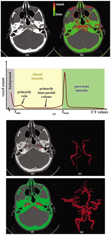
Result of carotid vessel segmentation in a patient's CTA. (a) An axial image slice. (b) Intensity based characterization of pure bone (green) and shared intensity band with red indicating high likelihood for vessels. (c) CTA intensity histogram with Imin and Ibone segmenting the background and the pure bone regions. (d) Axial image slice with the core vasculature marked in red. (e) 3-D rendering of the core vasculature. (f, g) 2-D and 3-D displays of bone-vessel separation using the MSO algorithm.
By taking the average of these values from three independent users on three CTAs, we selected Imin = 130Hu and Ibone = 500Hu and applied these values on all CTAs used in our experiments. It may further be mentioned that both soft bones and bone partial volume share the intensity band [Imin, Ibone] with vascular trees in CTAs (see Fig. 5(b)) and the objective of multi-scale opening is to separate bone and vessels over this shared intensity band. For the current experiment, the core vessel intensity Ivessel was set at Imin and the fuzzy membership functions μbone and μvessel were computed following Equations 9 and 10. Since the pure intensity zone for vessel was empty, no intensity value-defined seed voxels was used for vessels. For the bone structure, two types of seed voxels were used as follows:
boneSeedintensity: The set of voxels with their intensity values greater than or equal to Ibone.
boneSeedmanual: The set of bone seed voxels interactively indicated using a custom built graphical user interface.
Manual bone seed voxels were used for soft bones near sinus cavities. For each CTA, approximately 8 to 12 seed voxels were manually selected. Following the fact that no intensity based seed voxels may be used for vessels, we adopted a fuzzy connectivity and distance transform based approach to generate core vessels from a small set of user-specified vessel seed voxels. Let vesselSeedmanual be the set of manually indicated seed voxels for carotid vessels; in our experiments 8 to 12 manual seed voxels were added using our 2-D/3-D graphical interface. A fuzzy representation for vessels was computed from CTA using the membership function of Equation 10.
An FDT image Ωvessel : Ƶ3 → ℛ+ of vascular structures was computed from the fuzzy vessel image with the membership function μvessel : Ƶ3 → ℛ+. Let γvessel : Ƶ3 × Ƶ3 → ℛ+ denote the morpho-connectivity between two voxels as defined by Ωvessel. Using the manual vessel seed voxels vesselSeedmanual, a fuzzy morpho-connected vasculature image ϒvessel : Ƶ3 → ℛ+ was computed as follows:
| (11) |
It may be noted that the domain of ϒvessel expands into soft bones and partial volume bone voxels and to remove those from the core vessels we used morphological erosion by setting a threshold of 1.5 on ϒvessel. Here, the threshold value of 1.5 on ϒvessel indicate an erosion by 1.5 voxel units, i.e., ∼0.6 mm as the FDT image was computed in the voxel unit. Thus, vessels with diameter greater than 1.2 mm diameter survived as core vessel. Although the threshold value was empirically selected and may not be the optimum choice, it allowed successful disconnection of all soft bone and partial volume bone structures from the core vessel. A result of core vessel segmentation is illustrated in Fig. 5(d, e). Additional 8 to 12 separators (separatormanual) were manually selected and the MSO algorithm was applied to separate the entire vasculature (Fig. 5(f, g)) from bone. Results of bone/vessels separations for three other patients' CTA are illustrated in Fig. 6. Here, a half-skull representation of the carotid bone is adopted to display the vascular structure in the context of bone geometry.
Fig. 6.

Illustration of vascular segmentation results in three patients' CTAs. Here the bone structure is illustrated with partial transparency to depict segmented vessels through soft bones.
The performance of our method was compared with two existing algorithms [26]–[28], [30], [36]–[38]. The first algorithm was based on the method presented by Frangi and colleagues [26]–[28], [30]. It combines three popular concepts – Frangi's multi-scale vessel enhancement filtering [47], minimal cost-path using marching [48], and geodesic active region propagation using level-sets [49]. First, the user-indicated vessel seeds are connected using minimum cost-paths on the vesselness field and the voxels on those paths are treated as seeds for the next step of active region propagation. During this step vessel volume is segmented using geodesic active region propagation using level-sets. Let us refer to this method as multi-scale vesselness geodesic active region (MSVGAR) algorithm. A result of application of MSVGAR on a CTA is presented in Fig. 7(c). Essentially, the active region based propagation step in MSVGAR radially expands the vessel region and the propagation along the vessel is limited as it often leads to uncontrolled leaking prior to reaching distant vessels. These issues of the algorithm were also discussed by the authors [26]–[28], [30]. The parameters for scale-range, step-size and the gradient strength in MSVGAR were determined following the protocol recommended by the authors [26]–[28], [30].
Fig. 7.

Illustration of comparative results of vessel segmentation in a patient's CTA data using different algorithms – (a,b) MSO, (c) MSVGAR, (d) IRFC-conservative, and (d) IRFC- generous.
The second method selected for comparison was based on the iterative relative fuzzy connectedness (IRFC) [36]–[38], which was developed for separating conjoined objects and was applied for A/V separation in MR angiograms [36]–[38]. IRFC separates two objects using an iterative approach of relative strength of fuzzy connectivity between two competing objects. The fuzzy connectivity utilizes both gradient as well as object intensity feature through the “affinity” function as discussed in [15], [35]. Different parameters for object intensity and gradient features were computed over manually thresholded regions for bone and vessel regions. Two different versions of the IRFC algorithm were used for comparison—(1) IRFC-conservative and (2) IRFC-generous. For IRFC-conservative, the object intensity and gradient parameters were computed over a conservatively thresholded vessel region that ensured exclusion of all bone regions. On the other hand, for IRFC-generous, the object intensity and gradient parameters were computed over a generously thresholded vessel region that ensured inclusion of all visible vessels. Results of application of IRFC-conservative and IRFC-generous algorithm on a CTA are presented in Fig. 7(d) and (e), respectively. As observed in Fig. 7(d) and (e), the IRFC methods under-performed both MSO and MSVGAR algorithms. The primary reason behind the underperformance of IRFC methods is the absence of any intensity gradient at conjoining locations between vessels and bones and the lack of use of morphologic features in IRFC. Thus, the performance of IRFC methods is essentially similar to connectivity analysis on thresholded regions.
1) Quantitative Evaluation
To quantitatively examine the accuracy of the MSO algorithm, we manually indicated carotid vessel voxels as well as bone voxels at the vicinity of carotid vessels to define the gold standard or the ground truth. We carefully selected ground truth vessel/bone voxels from both large- and small-scale vessel regions.
Vesseltrue: Three thousand vessel voxels were manually selected on each CTA dataset by picking isolated voxels on different image slices.
Bonetrue: Three thousand bone voxels were manually selected on each CTA dataset by picking isolated voxels at the vicinity but outside vessels on different image slices.
The set of voxels Vesseltrue was used to determine true positive (TP) and false negative (FN) while Bonetrue was used to determine true negative (TN) and false positive (FP). Let Vesselcomputed be the set of voxels obtained for vessels using the proposed algorithm. Note that, unlike Vesseltrue, Vesselcomputed contains a large number of voxels of order of 100 million representing a volumetric region. Accuracy, sensitivity and specificity measures were defined as follows:
| (12) |
| (13) |
| (14) |
True positive, true negative, false positive and false negative of MSO-based vessel segmentation on individual CTA images from ten human subjects are presented in Table I and the accuracy, sensitivity and specificity of vessel segmentation from these experimental results are summarized Table II. It is observed from Table II that an average accuracy of 96.3% is achievable with the sensitivity and specificity of 95.1% and 97.5% respectively. Also, the variation in performance among different CTA images was relatively small with the observed standard deviation for accuracy, sensitivity and specificity among different images being 2.1, 3.1, and 2.5, respectively. A similar trend was observed the minimum and maximum values of these performance measures among different images. Comparative results of accuracy, sensitivity and specificity of vessel segmentation on the ten CTAs using MSO and the three existing algorithm, namely, MSVGAR, IRFC-conservative and IRFC-generous, are presented in Table III. As observed in the table, MSO outperforms the three methods in terms of all three performance metrics—accuracy, sensitivity and specificity— and these results reconfirm the of comparative segmentation results illustrated in Fig. 7. It may be noted segmentation results using IRFC-conservative method yields low sensitivity, while those using IRFC-generous are attributed with low specificity. As discussed earlier, the formulation of IRFC based methods assume a gradient separator at conjoining locations between two object and the absence of such gradient separation in the current application leads to the poor performance of IRFC methods.
Table I. Results of True Positive (TP), True Negative (TN), False Positive (FP) and False Negative (FN) on Individual Ten Datasets.
| Data-ID | TP | TN | FP | FN |
|---|---|---|---|---|
| 1005 | 2514 | 2882 | 33 | 170 |
| 1016 | 2966 | 3067 | 33 | 60 |
| 2001 | 2088 | 2532 | 12 | 80 |
| 2005 | 2627 | 3548 | 75 | 120 |
| 2008 | 2166 | 2725 | 279 | 108 |
| 3029 | 2558 | 2977 | 85 | 191 |
| 3032 | 2102 | 2306 | 34 | 52 |
| 3036 | 2219 | 2316 | 130 | 108 |
| 4001 | 2326 | 2568 | 44 | 104 |
| 4002 | 2032 | 2482 | 120 | 118 |
Table II. Quantitative Results of Accuracy, Sensitivity and Specificity of the Developed MSO Algorithm for Ten Human CTA Datasets.
| Accuracy | Sensitivity | Specificity | |
|---|---|---|---|
| Average | 96.3 | 95.1 | 97.5 |
| Std. dev. | 2.1 | 3.1 | 2.5 |
| Min. | 91.6 | 88.6 | 91.8 |
| Max. | 98.4 | 98.6 | 99.7 |
Table III. Comparative Results of Accuracy, Sensitivity and Specificity of Vessel Segmentation on Ten Patients' CTA Data Sets Using Different Methods.
B. Reproducibility
In this section, we present our experimental methods and results evaluating the reproducibility of the MSO algorithm. A multi-user reproducibility analysis of vessel segmentation was performed on the same human CTA images described in accuracy experiment. Specifically, the reproducibility of vessel segmentation results from two mutually-blinded independent trained-users was examined. Eight to twelve seed voxels for each of the two objects and another 8 to 12 separators were manually added by two mutually blinded independent trained-users using our custom 2D/3D graphical interface and the results of carotid vessel segmentation were used for reproducibility analyses. 3D renditions of segmented vascular trees for two data sets by two different users are illustrated in Fig. 8. Vascular segmentation results generated by two mutually blinded trained-users for one dataset are shown in Fig. 8(a, b). Although the results are visually similar, differences are observed in some finer vessels. In the case of the other dataset, differences in vascular segmentation results are different at the bottom of the vascular tree (see Fig. 8(c, d)). This is mainly due to the choice of placement of seeds at those regions. Despite complex structure of cerebral vasculatures, for most datasets, segmentation results by two independent experts agree significantly. In order to quantitatively evaluate multiuser reproducibility of the method, we computed the following measure of agreement:
Fig. 8.

Results of vascular segmentation and bone removal in two patients' CTA data sets as obtained by two mutually blinded trained-users. Reproducibility results shown in the first row are visually almost indistinguishable due to high Agreement (96.9%), while the results in the bottom row have moderate Agreement (94.2%) with apparent differences in segmentation results near the bottom section of the arterial tree
| (15) |
where, Bi and Vi denote separated objects using seed voxels selected by the ith expert. Using two mutually blinded trained-user inputs, the MSO algorithm produced an average Agreement of 94.2±3.8%. The maximum and minimum values of Agreement observed in our experiment are 96.9% and 88.6%. Although agreement between two independent trained-users is generally high, there are some disagreements in object separations by two trained-users. It may be noted that these results of reproducibility reflect the robustness of the entire process in the presence of human errors and effectiveness of the graphical interface.
C. Efficiency
Approximately, 25-35 seeds/separators were used for each CTA data through a custom graphical user interface (GUI) requiring an average of thirty minutes to complete carotid vascular segmentation in each CTA data. Current implementation of the MSO algorithm on a desktop with a 2.53-GHz Intel(R) Xeon(R) CPU and Linux OS requires approximately 10 minutes to complete the MSO computation on a patient's CTA data set excluding the user interface time through the GUI. The average computation time for one CTA data set using MSVGAR and IRFC algorithms on the same machine are 3 minutes and 5 minutes, respectively.
V. Conclusion
In this paper, the theoretical properties of the MSO algorithm for similar-intensity fuzzy objects have been established and a new algorithm has been presented for separating two conjoined fuzzy objects with different intensity characteristics while partially sharing a common intensity band, which are fused at different scales and locations. The current work extends our previous research [17], [19] on artery-vein separation in 3-D non-contrast pulmonary CT imaging which was formulated as a multi-scale separation task for two similar-intensity conjoined objects. Besides the establishment of new theoretical properties of the MSO algorithm, the key methodological contributions in the current work include—(1) modeling of multi-scale bone-vasculature separation problem for human CTA images, (2) GUI based practical solution to extract the carotid vascular tree with minimal user intervention, and (3) opens a new avenue for effective separation of fuzzy objects over a shared intensity space. Results of application of the new algorithm to A/V separation in a physical cast phantom of a pig lung have been illustrated. Accuracy and reproducibility of the algorithm in segmenting carotid vasculature in patients' CTAs have been examined and the results have been presented. Overall, high accuracy and reproducibility were observed in our experimental results. High accuracy and reproducibility at the cost of moderate user efforts demonstrates that the algorithm is suitable for application to clinical and research studies involving pulmonary A/V separation and human CT angiography.
The performance of the new method in terms of accuracy, sensitivity and specificity of carotid vessel segmentation in patients' CTAs was compared with three existing methods and the results are presented. The current methods outperform all three methods with respect to all the three performance metrics. Visual segmentation results show that, while MSVGAR generates acceptable results in segmentation the local vascular structure, its ability to propagate along vessels without leaking into bones is limited. The performance of IRFC methods in the current application was lower relative to both MSO and MSGVGAR algorithms. The computational complexity of the current method is somewhat higher than existing methods due to repeated computation of FDT at the beginning of the algorithm as well as during constrained dilation in each iteration. Currently, we are working on improving computational efficiency of the MSO algorithm using parallelization and ideas related to locally-confined efficient computation of FDT for iterative constrained dilation.
This method may be applied to generate an augmented virtual reality environment where the segmented arterial tree obtained using our algorithm may be mapped onto low-resolution dynamic CT images to interactively guide a surgeon in reaching an aneurysm along the optimum pathway in the cerebral arterial tree in the actual patient coordinate system. Our future plan is to develop such an environment using our algorithm that will maximally utilize smart graphical user interface, parallel processing and ultra-low dose imaging of modern CT scanner.
Acknowledgments
Authors are grateful to Dr. Robert E. Harbaugh, Penn State Hershey Medical Center and Dr. Madhavan L. Raghavan, Department of Biomedical Engineering, University of Iowa for sharing the CTA datasets used in this study.
This work was supported in part by NIH grants R01-AR054439 and R01-HL112986. Research work of Subhadip Basu was supported by the BOYSCAST fellowship (SR/BY/E-15/09) and FASTTRACK grant (SR/FTP/ETA-04/2012) by DST, Government of India.
Biographies
Punam K Saha is a professor of Electrical and Computer Engineering and Radiology at the University of Iowa. He is the director of the Structural Imaging Laboratory at the University of Iowa. He received his Ph.D. degree in 1997 from the Indian Statistical Institute, where he served as a faculty member during 1993-97. In 1997, he joined the University of Pennsylvania as a postdoctoral fellow, where he served as a Research Assistant Professor during 2001-06, and moved to the University of Iowa in 2006. His research interests include image processing, segmentation and analyses, trabecular bone imaging, quantitative structural assessment in medical imaging. He has published over 95 papers in international journals and over 300 papers/abstracts in international conferences, and holds numerous patents related to medical imaging applications. He received a Young Scientist award from the Indian Science Congress Association in 1996. He has served as an associate editor for Pattern Recognition and Computerized Medical Imaging and Graphics journals; currently, he is an Associate Editor of the IEEE Transactions on Biomedical Engineering and the Pattern Recognition Letters journal. He has served in many international conferences at various levels. He has received several grant awards from the National Institute of Health, USA.

Subhadip Basu is an Assistant Professor in the Department of Computer Science and Engineering, Jadavpur University, Kolkata, India since 2006. He received his Bachelor of Engineering degree in Computer Science and Engineering in 1999 and his Ph.D. (Engineering) degree in 2006. He did his post-doctoral researches in Hitachi Central Research Laboratory, Japan, University of Warsaw, Poland and in the University of Iowa, USA. Dr. Basu has published more than 130 research articles in various International Journals, Conference proceedings and book chapters on various applications of Pattern Recognition and image analysis. He has co-authored/edited five books and co-invented two US patents. He is the recipient of UGC Research Award, BOYSCAST and FASTTRACK young scientist fellowships from Govt. of India, HIVIP fellowship from Hitachi, Japan and EMMA fellowship from the European Union. He is a senior member of IEEE.

Eric A Hoffman is a professor of radiology, medicine and biomedical engineering at the University of Iowa. He is the director of the Advanced Pulmonary Physiomic Imaging Laboratory (APPIL) in the Department of Radiology and the director of the Iowa Comprehensive Lung Imaging Center (IClic) at the University of Iowa. He received his Ph.D. in Physiology from the University of Minnesota / Mayo Graduate School of Medicine in 1981 and remained on staff at the Mayo Clinic where he was a member of the team which developed the earliest volumetric CT scanner, the Dynamic Spatial Reconstructor (DSR). In 1987 he joined the faculty of Radiology at the University of Pennsylvania where he was the director of Cardiothoracic Imaging Research Center and moved to the University of Iowa in 1992. Dr. Hoffman is a fellow of the American Institute for Medical and Biomedical Engineering, an honorary lifetime member of the Society of Thoracic Radiology, a member of the Fleischner Society, and founder of the SPIE Medical Imaging track on Physiology and Function from Multidimensional Images. He has published more than 450 peer reviewed journal articles, numerous book chapters and review articles and holds numerous patents related to lung image analysis, CT contrast agents and respiratory synchronization devices. He recently received the 2014 Joseph R Rodarte Award for Scientific Distinction from the Respiratory Structure and Function Assembly of the American Thoracic Society and the 2013 John West award for Outstanding Contributions to the Field of Functional Pulmonary Imaging from the IWPFI. Dr. Hoffman's laboratory is dedicated to the use of advanced imaging methodologies for the exploration of normal and pathologic physiology of the lung. At the core of his laboratory is a state-of-the-art multi-spectral CT research facility.
Contributor Information
Punam K. Saha, Email: pksaha@engineering.uiowa.edu.
Subhadip Basu, Email: subhadip@cse.jdvu.ac.in.
Eric A. Hoffman, Email: Eric-hoffman@uiowa.edu.
References
- 1.Bushberg JT, Seibert JA, Leidholdt EM, Jr, Boone JM. The Essential Physics of Medical Imaging. Philadelphia, PA: Lippincott Williams & Wilkins; 2011. [Google Scholar]
- 2.Cho ZH, Jones JP, Singh M. Foundation of Medical Imaging. New York: Wiley; 1993. [Google Scholar]
- 3.Saha PK, Chaudhuri BB, Majumder DD. A new shape preserving parallel thinning algorithm for 3D digital images. Pat Recog. 1997;30:1939–1955. [Google Scholar]
- 4.Saha PK, Strand R, Borgefors G. Digital topology and geometry in medical imaging: A survey. IEEE Trans Med Imag. 2015;34(9):1940–1964. doi: 10.1109/TMI.2015.2417112. [DOI] [PubMed] [Google Scholar]
- 5.Saha PK, Borgefors G, Sanniti di Baja G. A survey on skeletonization algorithms and their applications. Pat Recog Lett. in press. [Google Scholar]
- 6.Sonka M, Fitzpatrick JM. Handbook of Medical Imaging, Volume 2 Medical Image Processing and Analysis. Bellingham, WA: SPIE Press; 2000. [Google Scholar]
- 7.Sonka M, Hlavac V, Boyle R. Image Processing, Analysis, and Machine Vision. 3rd. Toronto, Canada: Thomson Engineering; 2007. [Google Scholar]
- 8.Udupa JK, Herman GT. 3D Imaging in Medicine. Boca Raton, FL: CRC Press; 1991. [Google Scholar]
- 9.Bezdek JC, Hall LO, Clarke LP. Review of MR image segmentation techniques using pattern recognition. Med Phys. 1993;20(4):1033–48. doi: 10.1118/1.597000. [DOI] [PubMed] [Google Scholar]
- 10.Falca˜o AX, Stolfi J, de Alencar Lotufo R. The image foresting transform: Theory, algorithms, and applications. IEEE Trans Patt Anal Mach Intell. 2004;26(1):19–29. doi: 10.1109/tpami.2004.1261076. [DOI] [PubMed] [Google Scholar]
- 11.Heimann T, Meinzer HP. Statistical shape models for 3D medical image segmentation: a review. Med Image Anal. 2009;13(4):543–63. doi: 10.1016/j.media.2009.05.004. [DOI] [PubMed] [Google Scholar]
- 12.McInerney T, Terzopoulos D. Deformable models in medical image analysis: a survey. Med Image Anal. 1996;1(2):91–108. doi: 10.1016/s1361-8415(96)80007-7. [DOI] [PubMed] [Google Scholar]
- 13.Olabarriaga SD, Smeulders AW. Interaction in the segmentation of medical images: a survey. Med Image Anal. 2001;5(2):127–42. doi: 10.1016/s1361-8415(00)00041-4. [DOI] [PubMed] [Google Scholar]
- 14.Pham DL, Xu C, Prince JL. Current methods in medical image segmentation. Annu Rev Biomed Eng. 2000;2:315–37. doi: 10.1146/annurev.bioeng.2.1.315. [DOI] [PubMed] [Google Scholar]
- 15.Saha PK, Udupa JK, Odhner D. Scale-based fuzzy connected image segmentation: Theory, algorithms, and validation. Comp Vis Imag Und. 2000;77:145–174. [Google Scholar]
- 16.Lei T, Udupa JK, Saha PK, Odhner D. Artery-vein separation via MRA – an image processing approach. IEEE Trans Med Imag. 2001;20:689–703. doi: 10.1109/42.938238. [DOI] [PubMed] [Google Scholar]
- 17.Saha PK, Gao Z, Alford SK, Sonka M, Hoffman EA. Topomorphologic separation of fused isointensity objects via multiscale opening: Separating arteries and veins in 3-D pulmonary CT. IEEE Trans Med Imag. 2010;29(3):840–851. doi: 10.1109/TMI.2009.2038224. [DOI] [PMC free article] [PubMed] [Google Scholar]
- 18.Vasilescu DM, Gao Z, Saha PK, Yin L, Wang G, Haefeli-Bleuer B, Ochs M, Weibel ER, Hoffman EA. Assessment of morphometry of pulmonary acini in mouse lungs by nondestructive imaging using multiscale microcomputed tomography. Proc Natl Acad Sci USA. 2012;109(42):17105–10. doi: 10.1073/pnas.1215112109. [DOI] [PMC free article] [PubMed] [Google Scholar]
- 19.Gao Z, Grout R, Holtze C, Hoffman EA, Saha PK. A new paradigm of interactive artery/vein separation in non-contrast pulmonary CT imaging using multi-scale topo-morphologic opening. IEEE Trans Biomed Eng. 2012;59(11):3016–3027. doi: 10.1109/TBME.2012.2212894. [DOI] [PMC free article] [PubMed] [Google Scholar]
- 20.Brisman JL, Song JK, Newell DW. Cerebral aneurysms. New Engl J Med. 2006;355(9):928–939. doi: 10.1056/NEJMra052760. [DOI] [PubMed] [Google Scholar]
- 21.Kayembe K, Sasahara M, Hazama F. Cerebral aneurysms and variations in the circle of willis. Stroke. 1984;15(5):846–850. doi: 10.1161/01.str.15.5.846. [DOI] [PubMed] [Google Scholar]
- 22.Alberico RA, Patel M, Casey S, Jacobs B, Maguire W, Decker R. Evaluation of the circle of Willis with three-dimensional CT angiography in patients with suspected intracranial aneurysms. American J Neurorad. 1995;16(8):1571–1578. [PMC free article] [PubMed] [Google Scholar]
- 23.Abrahams JM, Saha PK, Hurst RW, LeRoux PD, Udupa JK. Three-dimensional bone-free rendering of the cerebral circulation by use of computed tomographic angiography and fuzzy connectedness. Neurosurgery. 2002;51(1):264–269. doi: 10.1097/00006123-200207000-00044. [DOI] [PubMed] [Google Scholar]
- 24.Josephson SA, Bryant SO, Mak HK, Johnston SC, Dillon WP, Smith WS. Evaluation of carotid stenosis using CT angiography in the initial evaluation of stroke and TIA. Neurology. 2004;63(3):457–460. doi: 10.1212/01.wnl.0000135154.53953.2c. [DOI] [PubMed] [Google Scholar]
- 25.Prokop M. Multislice CT angiography. Europe J Rad. 2000;36(2):86–96. doi: 10.1016/s0720-048x(00)00271-0. [DOI] [PubMed] [Google Scholar]
- 26.Cebral JR, Castro M, Appanaboyina S, Putman CM, Millan D, Frangi AF. Efficient pipeline for image-based patient-specific analysis of cerebral aneurysm hemodynamics: technique and sensitivity. IEEE Trans Med Imag. 2005;24(4):457–467. doi: 10.1109/tmi.2005.844159. [DOI] [PubMed] [Google Scholar]
- 27.Milla´n RD, Dempere-Marco L, Pozo JM, Cebral JR, Frangi AF. Morphological characterization of intracranial aneurysms using 3-D moment invariants. IEEE Trans Med Imag. 2007;26(9):1270–1282. doi: 10.1109/TMI.2007.901008. [DOI] [PubMed] [Google Scholar]
- 28.Radaelli AG, Augsburger L, Cebral JR, Ohta M, Rfenacht DA, Balossino R, Benndorf G, Hose DR, Marzo A, Metcalfe R. Reproducibility of haemodynamical simulations in a subject-specific stented aneurysm modela report on the Virtual Intracranial Stenting Challenge 2007. J Biomech. 2008;41(10):2069–2081. doi: 10.1016/j.jbiomech.2008.04.035. [DOI] [PubMed] [Google Scholar]
- 29.Steinman DA, Milner JS, Norley CJ, Lownie SP, Holdsworth DW. Image-based computational simulation of flow dynamics in a giant intracranial aneurysm. American J Neurorad. 2003;24(4):559–566. [PMC free article] [PubMed] [Google Scholar]
- 30.Zhang C, Villa-Uriol MC, De Craene M, Pozo JM, Frangi AF. Morphodynamic analysis of cerebral aneurysm pulsation from time-resolved rotational angiography. IEEE Trans Med Imag. 2009;28(7):1105–1116. doi: 10.1109/TMI.2009.2012405. [DOI] [PubMed] [Google Scholar]
- 31.Basu S, Raghavan ML, Hoffman E, Saha PK. Int Conf Intel Comput Bio-Med Instru (ICBMI) IEEE; 2011. Multi-scale opening of conjoined structures with shared intensities: methods and applications; pp. 128–131. [Google Scholar]
- 32.Saha PK, Wehrli FW, Gomberg BR. Fuzzy distance transform: Theory, algorithms, and applications. Comp Vis Imag Und. 2002;86:171–190. [Google Scholar]
- 33.Saha PK, Wehrli FW. Measurement of trabecular bone thickness in the limited resolution regime of in vivo MRI by fuzzy distance transform. IEEE Trans Med Imag. 2004;23:53–62. doi: 10.1109/TMI.2003.819925. [DOI] [PubMed] [Google Scholar]
- 34.Saha PK, Xu Y, Duan H, Heiner A, Liang G. Volumetric topological analysis: A novel approach for trabecular bone classification on the continuum between plates and rods. IEEE Trans Med Imag. 2010;29(11):1821–1838. doi: 10.1109/TMI.2010.2050779. [DOI] [PMC free article] [PubMed] [Google Scholar]
- 35.Udupa JK, Saha PK. Fuzzy connectedness and image segmentation. Proc of the IEEE. 2003;91:1649–1669. [Google Scholar]
- 36.Ciesielski KC, Udupa JK, Saha PK, Zhuge Y. Iterative relative fuzzy connectedness for multiple objects with multiple seeds. Comp Vis Imag Und. 2007;107:160–182. doi: 10.1016/j.cviu.2006.10.005. [DOI] [PMC free article] [PubMed] [Google Scholar]
- 37.Saha PK, Udupa JK. IEEE Work Math Meth Biomed Imag Anal. Hilton Head, South Carolina: 2000. Iterative relative fuzzy connectedness and object definition: Theory, algorithms, and applications in image segmentation. [Google Scholar]
- 38.Udupa JK, Saha PK, Lotufo RA. Relative fuzzy connectedness and object definition: Theory, algorithms, and applications in image segmentation. IEEE Trans Patt Anal Mach Intell. 2002;24:1485–1500. [Google Scholar]
- 39.Saha PK, Chaudhuri BB. 3D digital topology under binary transformation with applications. Comp Vis Imag Und. 1996;63:418–429. [Google Scholar]
- 40.Otsu N. A threshold selection methods from grey-level histograms. IEEE Trans Patt Anal Mach Intel. 1979;9:62–66. [Google Scholar]
- 41.Saha PK, Udupa J. Optimum threshold selection using class uncertainty and region homogeneity. IEEE Trans Patt Anal Mach Intel. 2001;23:689–706. [Google Scholar]
- 42.Kong TY, Rosenfeld A. Digital topology: Introduction and survey. Comp Vis Graph Imag Proc. 1989;48:357–393. [Google Scholar]
- 43.Saha PK, Chaudhuri BB. Detection of 3-D simple points for topology preserving transformations with application to thinning. IEEE Trans Patt Anal Mach Intell. 1994;16:1028–1032. [Google Scholar]
- 44.Bloch I. Fuzzy connectivity and mathematical morphology. Pattern Recognition Letters. 1993;14(6):483–488. [Google Scholar]
- 45.Rosenfeld A. Fuzzy digital topology. Info Contr. 1979;40:76–87. [Google Scholar]
- 46.Udupa JK, Samarasekera S. Fuzzy connectedness and object definition: Theory, algorithms, and applications in image segmentation. Graph Mod Imag Proc. 1996;58:246–261. [Google Scholar]
- 47.Frangi AF, Niessen WJ, Vincken KL, Viergever MA. Med Imag Comput Comput-Assist Interv (MICCAI'98) LNCS-1496. Springer; 1998. Multi-scale vessel enhancement filtering; pp. 130–137. [Google Scholar]
- 48.Sethian JA. Level Set Methods and Fast Marching Methods. Cambridge University Press; 1996. [Google Scholar]
- 49.Malladi R, Sethian JA, Vemuri BC. Shape modeling with front propagation: A level set approach. IEEE Trans Patt Anal Mach Intel. 1995;17:158–175. [Google Scholar]