Assessing the performance of different DTI motion correction strategies in the presence of EPI distortion correction

Abstract

Diffusion tensor imaging (DTI) is susceptible to several artifacts due to eddy currents, echo planar imaging (EPI) distortion and subject motion. While several techniques correct for individual distortion effects, no optimal combination of DTI acquisition and processing has been determined. Here, the effects of several motion correction techniques are investigated while also correcting for EPI distortion: prospective correction, using navigation; retrospective correction, using two different popular packages (FSL and TORTOISE); and the combination of both methods. Data from a pediatric group that exhibited incidental motion in varying degrees are analyzed. Comparisons are carried while implementing eddy current and EPI distortion correction. DTI parameter distributions, white matter (WM) maps and probabilistic tractography are examined. The importance of prospective correction during data acquisition is demonstrated. In contrast to some previous studies, results also show that the inclusion of retrospective processing also improved ellipsoid fits and both the sensitivity and specificity of group tractographic results, even for navigated data. Matches with anatomical WM maps are highest throughout the brain for data that have been both navigated and processed using TORTOISE. The inclusion of both prospective and retrospective motion correction with EPI distortion correction is important for DTI analysis, particularly when studying subject populations that are prone to motion. Hum Brain Mapp 37:4405–4424, 2016. © 2016 Wiley Periodicals, Inc.

INTRODUCTION

Image quality in any magnetic resonance imaging (MRI) modality depends significantly on both the data acquisition methods (i.e., the implemented pulse sequences) and the subsequent processing steps utilized. In diffusion tensor imaging (DTI) most standard pulse sequences are based on single‐shot echo planar imaging (EPI) for reading out the MRI signal. The diffusion weighted imaging (DWI) data can be adversely affected by a combination of several artifacts due to the implementation of strong diffusion gradients to probe water diffusion and EPI schemes and to allow for fast acquisition [Le Bihan et al., 2006]. Artifacts include eddy currents induced mainly by switching the DW gradients on and off, EPI distortions induced by magnetic field (B0) inhomogeneity and subject motion [Ardekani and Sinha, 2005; Irfanoglu et al., 2012; Jezzard et al., 1998; Landman et al., 2007; Wu et al., 2008].

Complications in correcting these effects arise due to the fact that each DW volume has a different diffusion contrast, as well as relatively low signal‐to‐noise ratio (SNR). Several MRI pulse sequences for prospective (real‐time) distortion correction have been designed to minimize the effects of eddy currents [Reese et al., 2003], subject motion [Alhamud et al., 2012; Benner et al., 2011; Kober et al., 2012] and EPI distortion [Alhamud et al., 2016; Holland et al., 2010]. However, these sequences either may not be available on most MRI scanners or are not able to fully correct for all distortions. Therefore, several retrospective correction methods for the above distortions have been designed as an alternative means to correct or add more accuracy in the prospectively corrected data, for example, see [Andersson et al., 2003; Irfanoglu et al., 2012; Landman et al., 2007; Mukherjee et al., 2008; Rohde et al., 2004; Wu et al., 2008]. To date, however, no optimal combination of DTI acquisition and processing has been definitively determined, and the purpose of this manuscript is to assess the efficacy of one such prospective motion correction technique together with two well‐known postprocessing methods.

The process of combining correction methods is inherently complicated: there are a wide variety of techniques to choose from for each step; the effects of each distortion are not fully independent; and, similarly, the actions of each correction technique are not independent. For example, B0 distortion causes both spatial shifts and geometrical distortions of imaged objects, particularly along the phase‐encoding direction, as well as intensity variation; subject motion also results in spatial shifts, and eddy currents produce severe geometric distortion, especially in DTI images. Most processing steps depend on some form of volume alignment, such as of DWIs to a reference non‐weighted (b ₀) or anatomical volume for example, [Rohde et al., 2004], and therefore, the effects of subject motion (and any correction steps taken) become convolved in and influence the quality of all other analysis procedures and results [Aksoy et al., 2008; Landman et al., 2007; Ling et al., 2012; Norris, 2001]. Additionally, computational processing techniques, which are often nonlinear and based on model assumptions, may introduce nonphysiological factors into the outcomes, such as warping, smoothing, or the modeling of noise as signal. Research remains active in this area, particularly as diffusion imaging becomes increasingly applied in clinical settings and in younger populations, who are highly prone to motion, and using greater magnetic field strengths and higher diffusion weighting (DW) factors, such as in high angular resolution diffusion imaging techniques, both of which increase the potential for nonlinear effects [Cole et al., 2014; Dubois et al., 2014; Elhabian et al., 2014; Kong et al., 2014; Kreilkamp et al., 2016; Tijssen et al., 2009].

In this study, we investigate the effects of using different motion correction techniques within complete DTI processing pipelines that include eddy current and EPI distortion correction. In particular, we examine utilizing: (1) prospective motion correction in real‐time during data acquisition; (2) retrospective correction using various computational techniques for volume registration; and (3) the combination of both prospective and retrospective methods. Previous DTI studies have compared the use of prospective and retrospective correction algorithms and reported that the latter tend to result in a significant reduction in fractional anisotropy (FA) parameter values in both gray matter (GM) and white matter (WM), even in the absence of subject motion and for a stationary phantom [Alhamud et al., 2012, 2015]. However, these studies performed motion correction with only one technique, and they also did not look at the inclusion of retrospective correction in conjunction with EPI distortion correction, which has been shown to be important in diffusion scanning [Irfanoglu et al., 2012].

In the present study, we use two DTI acquisition methods (with and without prospective (real‐time) subject motion correction during scanning) and two processing pipelines to analyze combinations of prospective and retrospective distortion correcting techniques. This includes comparing two popular, publicly available diffusion‐processing tools, [Smith et al., 2004], and TORTOISE [Pierpaoli et al., 2010], for retrospectively correcting distortion effects (subject motion, eddy currents, and EPI distortion). We hypothesize that, depending on the specific method, retrospective motion correction can be combined beneficially with prospective motion correction (e.g., using navigators) in order to improve final results of full DTI processing. By analyzing results of processing pipelines with and without explicit retrospective motion correction, one may approximately estimate the size of the effect of its inclusion. To compare the pipeline results, we use both quantitative and qualitative examinations of DTI parameters and probabilistic tractography. Differences between full processing pipelines, depending on the data acquisition and software used, are also presented and discussed. The analyzed group is comprised of pediatric subjects (approximately 7 years of age), as children are likely to engage in incidental motion throughout a scanning session, providing a particular challenge for any data acquisition and analysis [Holdsworth et al., 2012; Theys et al., 2014].

METHODS

Data Acquisition

Six healthy children (4F/2M, age 7.20 ± 0.06 years) were scanned without sedation as part of an ongoing study using an Allegra 3T MRI (Siemens Healthcare, Erlangen, Germany) in Cape Town, South Africa. Subjects were instructed not to move during scanning, though incidental motion occurred (as expected, given the ages of the subjects). Human subjects approval was obtained from the Human Research Ethics Committees of the University of Cape Town Faculty of Health Sciences and Stellenbosch University. Parents/guardians provided written informed consent and children provided oral assent at the time of scanning.

The following whole brain (WB) data were acquired for each subject, as determined by the ongoing study's protocols. A T1‐weighted (T1w) anatomical image was acquired in the sagittal plane using a navigated multiecho magnetization prepared rapid gradient echo (MEMPRAGE) sequence [Tisdall et al., 2009; van der Kouwe et al., 2008]: voxel = 1.3 × 1 × 1 mm³, FOV = 224 × 224 × 144 mm³, matrix size 168 × 224 × 144, TR = 2,530 ms, TEs = (1.53, 3.19, 4.86, 6.53) ms, TI = 1,100 ms, flip angle = 7°. A standard DTI set was acquired using a twice refocused SE‐EPI sequence [Reese et al., 2003]: TR/TE = 9,500/86 ms, voxel = 1.964 × 1.964 × 2.000 mm³, FOV = 220 × 220 × 144 mm³, 4 b ₀ (b = 0 s/mm²) volumes and 30 noncollinear gradients with DW factor b = 1,000 s/mm². The DTI set consisted of a pair of acquisitions of opposite phase encodings (“AP‐PA”, acquired along anterior–posterior and posterior–anterior directions). Additionally, a navigated (vNav) DTI set was acquired using the same parameters as the standard set but with TR = 10,026 ms.

Briefly, the navigator was implemented as follows in order to track subject motion and to update the scanner gradient coordinates in real‐time. The standard twice‐refocused, 2D diffusion pulse sequence [Reese et al., 2003] had previously been modified to perform prospective motion correction by acquiring a single 3D, multishot EPI navigator (526 ms) following the acquisition of each diffusion volume [Alhamud et al., 2012]. As the navigator is not diffusion weighted, the accuracy of co‐registration and motion estimates are not affected by the diffusion gradients, even at high b‐values. Before the start of the subsequent diffusion volume, the navigated DTI sequence receives motion parameters resulting from the co‐registration of the current navigator to the reference navigator of the first diffusion volume. The rotation matrix, which depends on the slice orientation, is updated to the current position, then the matrix is used to reorient all spatial encoding gradients as well as the diffusion gradients. In this manner, the diffusion table for the next diffusion volume is kept in the correct slice orientation, and therefore the gradient table does not need to be reoriented retrospectively [Alhamud et al., 2012].

The 3D EPI navigator was implemented with a very small flip angle of 2° to minimize the impact of signal saturation on the diffusion sequence. For fast and efficient motion tracking, with minimal distortion, the navigator's protocol was implemented for each partition in the 3D slab with a low spatial resolution (8 × 8 × 8 mm³), with minimal TR (14 ms) and TE (6.6 ms) and with a very high receiver bandwidth (3,906 Hz/px). The reacquisition process was activated within the protocol, and up to five corrupted diffusion volumes were reacquired in‐line when motion exceeded preset thresholds for translation (>2.5 mm) or rotation (≥1°). The navigator would cease tracking in cases of translation >20 mm or rotation >8°. However, if less than five reacquisitions were activated, then the remaining reacquisitions were applied to the last volume. In each set of reacquired copies, only the last volume was kept for further processing.

Data Processing

Data were processed using a combination of TORTOISE [Pierpaoli et al., 2010], FSL [Smith et al., 2004], AFNI [Cox, 1996], FATCAT [Taylor and Saad, 2013], and in‐house scripts, as described below.

In preparation for DWI registration in TORTOISE, the T1w images were passed through an in‐house inversion algorithm to create a volume with approximate T2‐weighted (T2w) contrast (which is the recommended format for anatomical reference in this tool). A description of the algorithm, with example images, is shown in Appendix A. This T2w‐like volume was used solely for providing TORTOISE with an anatomical reference with requisite contrast similar to the DTI b ₀ volume, and it did not enter into any further step of processing or comparison. The FSL tools did not require an anatomical reference. Additionally, GM, WM and cerebrospinal fluid (CSF) tissue masks were calculated from the T1w images using AFNI‐3dSeg for later comparisons.

For comparison, the two primary DTI tools, FSL‐topup (v5.0.8) and TORTOISE (v2.1.0), were implemented separately in this study to provide post‐acquisition distortion correction for each diffusion data set. Prior to any processing, all diffusion data were visually inspected, and any corrupted volumes with signal dropout were removed. Then, FSL‐topup (TOP) was applied after FSL‐eddy_correct. Processing with TORTOISE (TORT) was performed separately in parallel using the DIFF_PREP and DR‐BUDDI tools.

For each processing tool default settings and steps provided by the software's basic help documentation were utilized. The final DWI data produced by the TORTOISE pipeline had 1.5 mm isotropic voxel resolution, as part of the standard settings, and the FSL output remained at 2 mm isotropic resolution. However, parameter distributions and WM maps were compared in each subject's 1 mm isotropic anatomical space, and tractography results were compared in the same standard template space (described below). In the final comparisons, there were, therefore, a total of four processed outputs per subject, each having: either Standard or vNav acquisition, and a standard implementation of either TOP or TORT tools. The labels for each describe the combined acquisition and processing, for example, “vNav_TOP” is a data set acquired using a navigator and processed with FSL‐topup; “TORT”' applies to both navigated and non‐navigated data sets that were processed in TORTOISE.

Analysis and Comparisons of Data

After processing, AFNI and FATCAT were used to average the b ₀ volumes of each data set (for TOP data; the TORT data had been averaged during processing), to fit diffusion tensors (DTs) nonlinearly and to calculate DTI parameters. Additionally, FA uncertainty, ΔFA, and the orientation uncertainty of the first eigenvector toward the orthogonal second and third eigenvectors, Δe ₁₂ and Δe ₁₃, respectively, were estimated using 3dDWUncert with 300 Monte Carlo iterations. FA maps were linearly warped to each subject's T1w anatomical space using six degrees of freedom (DOF) (rigid body parameters: three translation and three rotation). Distributions of FA and eigenvector parameters both within the WB and T1w‐segmented WM volumes were calculated; in previous studies, comparisons of FA distributions have been used to show the relative amounts of smoothing present in procedures, with more smoothing decreasing FA values (i.e., shifting the distribution leftward) in WM and increasing some FA values in GM (for the latter, particularly near tissue boundaries) [Alhamud et al., 2012; Kreilkamp et al., 2016]. Additionally, WM masks derived from DTI parameter values (where FA > 0.2, the standard proxy for WM in adult humans) were compared for overlap with T1w‐WM masks, both visually and quantitatively using Dice coefficients [Dice, 1945]. In order to examine how physiological noise and nonphysiological factors such as distortion vary throughout the image [Irfanoglu et al., 2012; Walker et al., 2011], the Dice coefficients were calculated separately for each coronal slice throughout the WB.

We also examined the basic alignment quantities calculated by each processing tool, for a comparison of processing features of the analysis tools themselves. Specifically, we investigated the values of the six rigid body registration parameters determined by each program. While each tool was implemented with more DOF in their alignment procedures (e.g., shearing and/or higher order terms), the exact implementations across the programs differ significantly, and therefore only these basic 6 DOF are directly comparable. We also calculated the root mean square (RMS) deviation for each subject, which combines the six rigid body parameters into a single estimator of mean displacement [Jenkinson, 1999; Reuter et al., 2015]:

$$\text{RMS}\hspace{0.17em}=\hspace{0.17em}\text{sqrt}\hspace{0.17em}\{r*r/5\hspace{0.17em}+\hspace{0.17em}\text{tr}\left[{\left(\mathbf{M}\hspace{0.17em}–\hspace{0.17em}\mathbf{I}\right)}^T\left(\mathbf{M}\hspace{0.17em}–\hspace{0.17em}\mathbf{I}\right)\right]\hspace{0.17em}+\hspace{0.17em}{\mathbf{t}}^T\mathbf{t}\},$$ (1)

where t is the translation vector, M is (here) the 3 × 3 rotation matrix, I is the identity matrix, tr[] is the trace operator, and r is the approximate spherical radius of the brain (here, estimated from the data to be 65 mm). The rigid body parameters and RMS values of the navigator logs were also examined.

In order to examine the practical consequences of DWI acquisition and processing, network tractography was performed, as this procedure simultaneously depends on ellipsoid orientation and shape, both locally and across regions of voxels. From the anatomical parcellation of the Haskins pediatric template [Molfese et al., 2015], 10 bilateral GM ROIs across the cerebral cortex and associated with the default mode network (DMN) were selected to form a network of targets: the left and right precuneus, posterior cingulate cortex, inferior parietal cortex, medial orbitofrontal cortex, and pars opercularis. This GM network was mapped nonlinearly to each subject's T1w anatomical using 3dQwarp, and then with a linear affine transform (12 DOF) to each subject's native diffusion space. Each region was inflated by one voxel in subject diffusion space using 3dROIMaker to ensure mapped regions maintained contact with FA > 0.2 WM (regions already within FA‐WM were not expanded, and target ROI overlap was prohibited). Probabilistic tracking was performed using 3dTrackID [Taylor and Saad, 2013; Taylor et al., 2012] with standard settings for all data sets: FA > 0.2 threshold; tract length >20 mm; turning angle <55°; N _seed = 5 tract seeds per voxel; N _MC = 1,000 Monte Carlo iterations; and a fractional threshold of f _tr = 0.05 (so that f _tr × N _seed × N _MC = 250 tracts/voxel were required for the voxel to be included in the final WM ROI). Tracking made use of the previously calculated DTI parameter uncertainty from 3dDWUncert.

Tracking results were compared for consistency by transforming the mask of each subject's intranetwork (AND‐logic, for greater within‐group consistency [Heiervang et al., 2006]) WM connections to the Haskins template space. The masks were added for each acquisition + processing pipeline, creating a group “summation map,” in which the voxel values contain the fraction of the group in which WM was found. In order to compare the relative sensitivity and specificity of the tracked results within the group, the following quantities were calculated within each summation map: the number of WM voxels as a function of group overlap (i.e., the number present in 100% of the group, the number in only 50%, etc.); and the fraction of voxels in each summation map as a function of group overlap (i.e., the preceding quantity scaled by the total size of the nonzero summation map).

RESULTS

Table 1 shows the numbers of DWIs in each subject's final set after removing any reacquired volumes or volumes with dropout slices. As expected, the size of the vNav set was typically (but not uniformly) greater than or equal to that of the Standard acquisition, as the former method had implemented reacquisition in case the navigator registered large subject motion (see Methods). Subjects “D” and “F” exhibited the most significant differences between Standard and vNav set size. During the vNav PA acquisition, subject “E” exhibited motion that exceeded navigator limits (>8° rotation), and therefore only the AP set was navigated for this subject.

Table 1.

Basic DTI set characteristics

	Subject ID
	A	B	C	D	E	F
NDWI
vNav	29	30	28	30	25	29
Standard	29	30	29	19	22	22
FA in WB (mean ± stdev)
vNav_TORT	0.23 ± 0.16	0.23 ± 0.15	0.22 ± 0.15	0.24 ± 0.16	0.25 ± 0.16	0.22 ± 0.15
vNav_TOP	0.21 ± 0.15	0.22 ± 0.14	0.18 ± 0.12	0.23 ± 0.15	0.23 ± 0.15	0.21 ± 0.14
Standard_TORT	0.22 ± 0.16	0.23 ± 0.15	0.22 ± 0.15	0.26 ± 0.15	0.27 ± 0.16	0.24 ± 0.16
Standard_TOP	0.20 ± 0.15	0.22 ± 0.14	0.20 ± 0.14	0.22 ± 0.14	0.23 ± 0.15	0.22 ± 0.14
FA in T1w‐WM (mean ± stdev)
vNav_TORT	0.36 ± 0.17	0.34 ± 0.17	0.33 ± 0.16	0.35 ± 0.18	0.36 ± 0.17	0.34 ± 0.18
vNav_TOP	0.32 ± 0.16	0.31 ± 0.16	0.25 ± 0.15	0.29 ± 0.18	0.33 ± 0.17	0.31 ± 0.16
Standard_TORT	0.36 ± 0.17	0.34 ± 0.17	0.33 ± 0.17	0.36 ± 0.17	0.37 ± 0.17	0.36 ± 0.17
Standard_TOP	0.32 ± 0.16	0.31 ± 0.16	0.27 ± 0.16	0.31 ± 0.16	0.29 ± 0.17	0.32 ± 0.17

The number of DWIs (N _DWI) in each subject's final, analyzed set is shown for both the vNav and Standard acquisitions. Additionally, the means and standard deviations (stdev) of FA values within WB and T1w‐WM distributions (see Fig. 1) are presented for each subject and processing stream. The Supporting Information provides tables of mean diffusivity (MD) and principal eigenvalue (L1) values.

Whole Brain and White Matter DTI Parameter Comparisons

Figure 1 displays normalized FA distributions for each of the six subjects (A–F) throughout the WB (upper panel) and within T1w‐WM (lower panel). The FA distribution mean and standard deviation values are also presented in Table 1; see the Supporting Information for tables of additional DTI parameter values of the mean diffusivity (MD) and principal eigenvalue (L1). In the WB case, the vNav_TORT distributions appear to be slightly left‐shifted with respect to the Standard_TORT ones for D‐F. Compared to TORT in C‐E, TOP distributions tend to be left‐shifted. Within the T1w‐WM, the vNav and Standard TORT distributions are nearly identical in each subject and are among the most right‐shifted.

Figure 1.

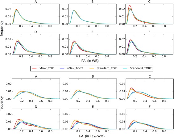
Normalized distributions of FA values in the WB (top) and in T1w‐WM (bottom) for all six subjects (A–F). In the WB cases Standard and TOP distributions tended to be the most rightward. In T1w‐WM TORT results were the least left‐shifted, suggesting that these sets had the least amount of smoothing. [Color figure can be viewed at http://wileyonlinelibrary.com]

Figure 2 displays the uncertainty distributions for the angular orientation of the DT's first eigenvector, with the mean (bias; upper panel) and standard deviation (stdev; lower panel) distributions of Δe ₁₂ plotted. All bias distributions have a peak around zero, with vNav data producing the narrowest linewidths for each of TOP and TORT. In the low‐motion cases “A‐C,” biases were similar across all methods; in “D‐F,” the Standard acquisitions showed the widest bias distributions. Similarly, the vNav‐acquired data showed the most left‐shifted peaks among stdev distributions, with vNav_TORT producing the highest peak at the smallest values.

Figure 2.

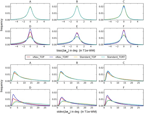
Normalized distributions of bias (top) and standard deviation (bottom) of the angular uncertainty, Δe ₁₂ (i.e., the first eigenvector projected along the second eigenvector), in T1w‐WM for the same subjects shown in Figure 1. [Color figure can be viewed at http://wileyonlinelibrary.com]

Figure 3 provides a quantitative comparison of the overlap of T1w‐ and FA‐WM maps, plotting Dice coefficients for each coronal slice in the brain volume. These direct measures were calculated for each coronal slice and then plotted along the anterior–posterior (i.e., phase‐encoding) axis, in order to highlight relative effects of EPI distortion in particular. The vNav_TORT data consistently showed the highest matches across the brain, and Standard_TORT were roughly equal or slightly lower. The vNav_TOP data often showed relatively high Dice values in the middle slices (excepting in C and D), which decreased quickly at the anterior and posterior edges.

Figure 3.

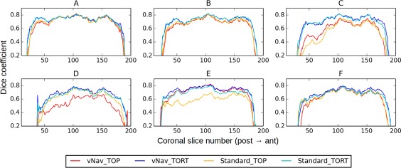
Dice coefficients of overlap between WM masks defined using FA and T1w images (same subjects as Figs. 1 and 2). Individual Dice coefficients were calculated for each coronal slice in the overlaid volumes. Dice values are relatively constant across the volumes, with vNav_TORT consistently showing the highest values. [Color figure can be viewed at http://wileyonlinelibrary.com]

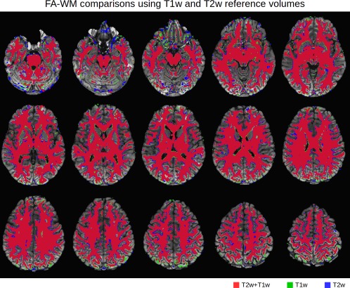
For examples of visual comparison, highlighting locations of mismatches due to either false negatives or positives, the relative overlaps for FA‐ and T1w‐WM masks are displayed for subjects F and C in Figures 4 and 5, respectively. Three axial slices are shown for each processed data set, with colors labelling relative matching of the FA‐WM to the reference T1w‐WM: direct overlap in red; false positives in green (i.e., regions incorrectly included as WM on FA masks); false negatives in blue (i.e., WM regions not present on FA masks). Consistent with the Dice coefficients in Figure 3, in subject 'F' the relative amount of overlap and false negatives/positives are generally similar across the data sets. The vNav acquisitions tend to show less false positive (green) than the respective Standard slices. Also in agreement with Figure 3, the anterior regions of the vNAV_TORT data show the greatest amount of overlap (red) with relatively little false positive/negative.

Figure 4.

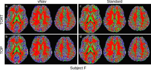
Comparison of FA (>0.2) and T1w (segmented) WM for subject “F,”, whose Dice coefficient curves were similar across acquisition and processing pipelines (Fig. 3). Locations where the FA‐WM overlaps with T1w‐WM are shown in red, with false positive and negative FA‐WM shown in green and blue, respectively. In each panel, the axial slices are arranged inferior (left) to superior (right). Standard images tend to show a relatively larger number of false positives. [Color figure can be viewed at http://wileyonlinelibrary.com]

Figure 5.

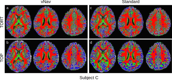
Comparison of FA (>0.2) and T1w (segmented) WM for subject C, whose Dice coefficient curves showed significant variation among the acquisition and processing pipelines (Fig. 3). Locations where the FA‐WM overlaps with T1w‐WM are shown in red, with false positive and negative FA‐WM shown in green and blue, respectively. In each panel the axial slices are arranged inferior (left) to superior (right). Standard TOP images show systematic differences in WM locations. [Color figure can be viewed at http://wileyonlinelibrary.com]

In contrast, for subject 'C' in Figure 5, there are much more extensive overlap differences among the different acquisition and processing methods. Standard_TOP shows large sections of false positives and negatives, particularly in the posterior regions, and vNav_TOP shows large regions of false negatives in lateral and anterior/posterior domains. Again, vNav_TORT shows the largest amount of direct overlap with the relatively smallest amount of false negatives and positives.

Motion Estimates During Acquisition and Processing

Figure 6 presents boxplots comparing (a) the six rigid body motion parameters calculated for all of the data sets and (b) the total RMS deviation for each subject. Values for each of the phase encoding sets (AP and PA) are shown separately. Rotation values were uniformly much smaller than translation (for example, converting rotation to length units with a rough approximation of a 65 mm head radius), particularly for rotation around the x‐axis. Translation in the z‐direction tended to have the largest parameter values. As observed in the RMS deviation, subjects “C,” “D,” and “E” appeared to have the largest overall registration values, suggesting that these subjects exhibited the largest motion.

Figure 6.

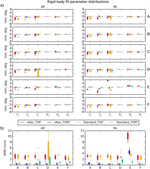
(a) Rigid body registration parameters (translation in mm and rotation in deg) for each subject as estimated by TOP and TORT programs. Results for each phase encoding direction (AP and PA) are shown separately. The mean of each distribution is shown with a black line, the color block covers the 25–75% interval, whiskers extend to 1.5× the interquartile range, and dots represent outliers. In nearly every case, the TOP distributions have the largest magnitude of mean and widest extent. (b) Distributions of the overall RMS deviations of the registration parameters are shown for each subject. Subjects “C,” “D,” and “E” exhibit the largest values; in the latter case, large registration values appear even in the navigated data set. [Color figure can be viewed at http://wileyonlinelibrary.com]

The magnitudes of motion correction parameter estimates differed greatly between the software tools. Typically, the mean magnitudes and ranges of estimated motion parameters were much higher for TOP processing than for TORT, in both the Standard and the vNav acquisitions and particularly for the translation parameters. Mean RMS values for TOP were greater than the voxel edge length (2 mm) for each set, while the mean for TORT surpassed that threshold for only one set (PA for “E”). For TOP, the means of the vNav RMS values were approximately greater than or equal to those of the Standard data in both the AP and PA sets for subjects “A,” “B,” “C,” and “D.” For TORT, the RMS means for vNav tended to be less than those of the Standard acquisition in the AP sets, and greater than or equal for most of the PA sets (though generally both were much less than 1 mm).

Additionally, the navigation logs of the vNav data were examined, for raw acquisitions as well as for a selected subset after reacquisition and visual inspection. Figure 7 shows the RMS values of the logs for all subjects, with the AP‐ and PA‐encoded sets shown separately (NB: the PA log file for subject “E” was not saved; the full times series of the logs are provided in the Supporting Information). Navigator values for all acquired volumes are shown in red; the subset excluding the volumes with large motion detected by the navigator (see Methods) are shown in black; and the final subset (used for analysis) which further excluded any volumes with dropout slices or without a matching AP and PA DW gradient are shown in cyan. These motion profiles are typical of incidental motion, generally being <1 mm with a small number of outliers. Subjects “C” and “E” showed the largest amounts of motion, including several outliers which were filtered out from the final DWI set used in the analyses.

Figure 7.

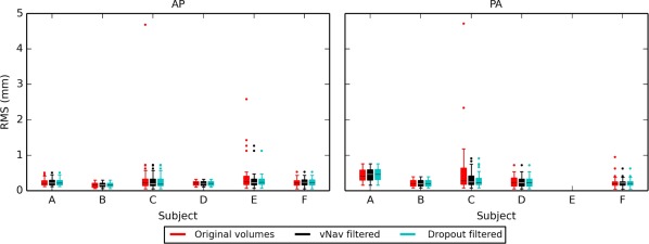
Overall RMS deviations of the rigid body subject motion parameters, as estimated by the navigator during data acquisition. Results for each phase encoding direction (AP and PA) are shown separately. Values for all acquired volumes are shown in red; volumes in black were kept after accounting for reacquisition (i.e., eliminating repetitions due either to excessive motion or post‐acquisition protocol; see Methods); and the set of cyan volumes were used for analysis after visual examination for dropout slices. Subjects “C” and “E” exhibited the largest amount of motion, with several outliers filtered out from each set for final analysis. [Color figure can be viewed at http://wileyonlinelibrary.com]

Tractographic Comparisons

In the final comparison of methods, probabilistic tractography was performed within each subject's native DWI space in order to determine pairwise connections among a default mode‐like network of target ROIs. For each acquisition + processing pipeline, each subject's mask of tracked WM was transformed to the standard Haskins pediatric template for the calculation of ‘summation maps’. Methods with greater specificity would produce fewer voxels with low percentages of overlap (i.e., exhibiting less heterogeneity); those with greater sensitivity would produce more voxels with 100% subject overlap (i.e., having the largest volume of group‐wide WM). Plots of the summation maps, as well as the target ROIs, are shown in sagittal slices in Figure 8. Locations of 100% overlap across the group are shown in red, while WM voxels found only for a single subject are shown in blue. Arrows highlight locations of high sensitivity for individual methods. For example, the cingulate bundles are most clearly specified across the group in the vNav_TORT case (panel “a,” first slice), as well as the inferior fronto‐occipital fasciculus (panel “a,” third slice).

Figure 8.

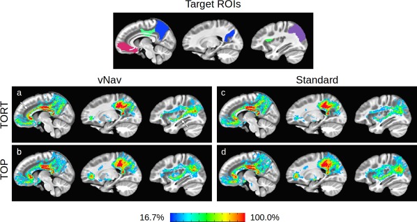
The top panel shows a map of the target ROIs (based on the DMN) in the same slice, with each cortex labeled with a unique color: medial orbitofrontal (red), posterior cingulate (green), precuneus (blue), and inferior parietal (violet). To examine the similarities and differences in tractographic results for each processing method, the mask of each subject's estimated intra‐network WM has been summed across the group in panels “a‐d.” Regions in the summation maps where all group members exhibited WM are shown in red, and regions where only one subject had WM are in blue. Locations of high sensitivity for individual methods are highlighted with magenta arrows. In each panel, sagittal images are arranged medial (left) to lateral (right). Quantitative comparisons of the summed masks are provided in Figure 9. [Color figure can be viewed at http://wileyonlinelibrary.com]

Figure 9 shows quantitative comparisons of the overlaps of estimated connections, plotting both the number of WM voxels (panel A) and the relative fraction of the nonzero WM (panel B) that is common to a percentage of the group. In both panels, TORT processed data, particularly with vNav acquisition, had the greatest specificity (i.e., lowest volume at lowest group overlap). The greatest sensitivity (i.e., the largest volumes with 100% overlap) was observed for Standard_TOP and vNav_TORT in panel A and for vNav_TORT in panel B.

Figure 9.

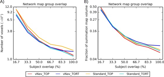
Quantitative comparisons of “summation maps” of tractographic results. All masks of intranetwork connections were mapped from each diffusion space to the Haskins pediatric template to create “summation maps” (shown in Fig. 8). Panel A shows the number of tracked voxels shared across a given percent of the group are shown. Panel B shows the same values, scaled by the number of nonzero values in the summation mask. [Color figure can be viewed at http://wileyonlinelibrary.com]

DISCUSSION

In this study, we have examined the effects of several motion correction techniques on DTI results, including: prospective correction using navigated acquisition; retrospective correction using computational registration; and their combination. We have used real data from a pediatric group who exhibited incidental motion in varying degrees, while also including processing steps for eddy current and EPI distortion correction. The estimated motion parameters, obtained both during acquisition (for navigated data) and from computational processing (for motion corrected data), were examined as part of the analysis. The goal of this study was not to compare specific software packages and implementations, but instead we aimed to examine the typical effects of prospective and retrospective motion correction techniques in DTI, as well as their combination, in conjunction with EPI distortion correction.

Combinations of Acquisition and Processing

It is difficult to differentiate the effects of subject motion from other confounding sources during acquisition and processing, including from any corrective technique itself [Ling et al., 2012; Norris, 2001]. All real data contain several nonphysiological factors such as eddy currents, magnetic field inhomogeneity, and scanner noise, none of whose contributions can be fully isolated. Therefore, any realistic study of motion correction must also take into account a full processing pipeline. This practical requirement informed the choice of software tools implemented in the present study; while several tools are publicly available for individual and multistep processing, we selected two standard, publicly available, and stand‐alone packages that each include tools for addressing subject motion, eddy currents and EPI susceptibility‐induced geometric distortions: FSL (eddy_correct and topup) and TORTOISE (DIFF_PREP and DR‐BUDDI). These are two of the most widely used software tools to explicitly combine these three correction aspects within a single pipeline.

Comparisons of DTI parameter distributions, WM maps and tractographic showed the importance of including prospective motion correction in diffusion studies. While results were typically similar between methods in cases of minimal subject motion, bias, and standard deviation of the ellipsoid orientation were uniformly smaller in navigated cases. The FA‐ and T1‐WM matches were highest across subjects and throughout the extent of the brain for vNav data processed with TORTOISE. Additionally, for tractography across the group of very similarly aged children, maps of the group's WM connections showed the greatest sensitivity and specificity for navigated data with TORTOISE processing. This result was consistent with the alignment of FA‐ and T1‐WM maps, where the same pipeline also produced the most consistent matches across the group. This is important for any practical diffusion study, where one wants to minimize effect of non‐neural factors on both within‐ and between‐group comparisons. In pediatric studies in particular, it is important to reduce the dependence of results on subject motion.

Prospective and Retrospective Motion Estimates

The results were examined in conjunction with quantities of subject motion measured during data acquisition (where available) and with those determined retrospectively by the processing algorithms. The subject motion profiles recorded by the navigator (vNav) logs were typical of incidental motion. There were generally minimal displacements and rotation, with a small number of instances of large motion (i.e., a significant fraction of voxel edge length or greater), and the greatest values tended to be either translation along the z‐axis or rotation around the y‐axis, which correspond to nodding of the head. While in vivo motion logs are not available from the scans acquired with the Standard method, it is assumed that the profiles would be qualitatively similar, given that the same subjects were scanned with both methods.

The TORT‐calculated rigid body registration parameters were typically similar to those of the navigator logs: a narrow distribution around zero, with a small number of outliers. For Standard data, the largest translations were along the z‐axis, and the largest rotations were along the y‐axis. Even after navigation, the registration parameters were not uniformly zero (though typically with a smaller mean than for the Standard data), often with 1–2 outliers. As the largest outliers were observed along the y‐axis, which was the direction of phase encoding, some may be associated with EPI distortions.

The distribution of the rigid body transformation parameters estimated by TOP had consistently larger means than those of TORT. In particular, the translation values were often greater than the edge length of a voxel, even in data that had been prospectively corrected with navigation and whose log profiles showed minimal movement. For TOP, the extent of the Standard and of the prospectively corrected vNav data were generally similar; in several cases, the mean registration values for the vNav data were larger than those of the Standard.

The non‐negligible values of the registration parameters across all data suggest that retrospective motion correction plays an important role in the processing, both for alignment and for further distortion correction as the amount of residual motion is decreased [Alhamud et al., 2012]. The prospective navigator used in the current study utilizes a rapid EPI acquisition with 8 mm isotropic voxels between DWIs, performing registration in real‐time and adjusting scanner coordinates [Alhamud et al., 2012]. While the navigator is able to report motion at the sub‐DTI voxel scale, it is likely that the retrospective correction with 2 mm voxels may provide additional alignment; in this case, the RMS values of retrospective TORTOISE correction were of order 0.5–1 mm, except in the event of very large subject motion. Moreover, subject motion will cause distortions in the B0 field, which cannot be corrected by real‐time correction alone. Thus, the retrospective correction in TORTOISE has a large effect to improve results for Standard data, and a smaller effect to improve results in the vNav data (most noticeably in the tractography results, as well as in the case of greatest subject motion).

Differences in Retrospective Correction Approaches

In both software pipelines initial motion correction is performed by registering each DWI to a reference b ₀ volume, though each method uses a different cost function for matching brightness patterns. Due to the contrast differences between each DWI with the b ₀ volume, FSL‐eddy_correct's default “inter‐modal” cost function for alignment is a correlation ratio. However, even in the near absence of subject motion, this method produced significantly nonzero registration parameter values (i.e., translations and rotations). The dispersion of each parameter distribution appeared to be strongly influenced by the varied brightness pattern of each volume (determined by the set of DW gradients, which was the same for each subject). That is, the matching of each DWI to b ₀ produced non‐negligible registration parameter values even in the absence of appreciable motion, due to how the inherent intensity differences were evaluated by the cost function, and the plotted distributions of each parameter's values were typically similar across the group, regardless of motion (excepting for translations along the z‐axis, where the most subject movement was observed). Thus, the TOP motion correction resulted in DT ellipsoids that were smoothed, even for small motion cases, as observed in the leftward shift of both the WB and T1‐WM FA distributions compared to the uncorrected fits, as well as in the lowered Dice coefficient values, consistent with results of other studies [Alhamud et al., 2012; Ling et al., 2012].

In contrast TORTOISE registration uses a normalized mutual information cost function, which minimally realigns DWIs in the absence of motion [Rohde et al., 2004]. This property was reflected in the observed registration parameters for data with small translations and rotations in the navigator logs. Moreover, the registration distributions varied across the group for a given parameter, suggesting that the alignment was less dependent on the contrast of each DWI.

An additional difference between the methods is that the TORT approach rotates the gradient table along with its motion correction steps, a step which the default TOP processing (used here; see the Methods) does not include, even though it has been recommended in previous DTI studies [Leemans and Jones, 2009]. However, it is likely that this feature was not a significant source of difference between the methods in the comparisons performed here, particularly in the scalar comparisons. The rotation parameters in the present registration steps (as well as in the navigation logs) were <2° (and generally <1°). Moreover, previous studies have shown that the effects of rotating the gradient table are small. For example, Leemans and Jones [2009] found that including gradient table rotation resulted in FA differences of the order of 10⁻⁴ and principal eigenvector differences of 2° for subject rotations of 3°, which is much larger than that observed in the current study. These marginal differences, particularly in FA, were much smaller than those observed between the TOP and TORT results. While small tensor errors are known to propagate through tractography [Lazar and Alexander, 2003], the expected differences due to gradient rotation were much smaller than the uncertainty distribution values for FA and eigenvector angles, which were used in the probabilistic tracking. This suggests that the larger differences between the TOP and TORT motion correction techniques would be the type of alignment used in each step (with the latter producing smaller values in cases of minimal motion); however, it may still be recommendable to insert a gradient rotation into the TOP pipeline, particularly in studies utilizing tractography.

An additional distinction between the methods is the use of an anatomical reference for distortion corrections in TORT, which may also play a critical role in reducing effects of distortions. Further technical differences between the methods are noted in Appendix B (as well as further comments on technical differences between acquisitions).

Limitations

An inherent limitation of the present study of motion correction techniques is that a large number of methodologies apply within each category of “prospective” and “retrospective” approaches, and not all of these may be examined. For example, Graham et al. (2016) have recently used simulated data to show that FSL‐eddy may be more effective than FSL‐eddy_correct in addressing DTI distortions, and so future work may examine this technique in a similar manner. Moreover, as noted above, the effects of subject motion and its correction in DTI cannot be isolated, as several other processing steps must be applied to address other distortion factors. Thus, we have used a selection of well‐tested motion correction techniques and used complete, existing pipelines for processing, even though the retrospective pipelines utilize different methods for addressing nonmotion distortion. The TOP method uses affine registration of DWIs to a reference b ₀ for correcting both subject motion and for the nonlinear eddy current distortions. In contrast, for motion and eddy current correction the TORT method uses both affine and quadratic terms (and a normalized mutual information cost function) to align each DWI to the b = 0 image, which itself is quadratically and nonlinearly aligned to the structural reference; the DWIs are warped into the structural space by the combination of these alignment steps [Irfanoglu et al., 2012; Rohde et al., 2004]. Thus, the present study is not a comprehensive comparison of motion correction techniques themselves, and further studies may continue to the issue of motion correction by using other processing implementations and new software.

CONCLUSIONS

This study has shown the benefits of including both prospective and retrospective motion correction in diffusion imaging studies, in addition to other distortion correction steps. Prospective correction has the benefits of updating (in real‐time) the scanner coordinate system to that of the subject, of allowing the reacquisition of volumes distorted by subject motion and of reducing the number of dropout volumes lost from a study, and significant benefit was seen in subjects with large motion during scanning. Certain retrospective motion correction can further improve volume alignment and aid in the net reduction of distortion during processing, particularly in cases of large subject motion. In the present tests full TORTOISE processing improved both standard and navigated DTI data, with the latter providing the best overall results. Combinations of prospective and retrospective motion correction can aid overall distortion correction, improve DT ellipsoid fits, and reduce variance in both local FA and tractographic results due to non‐physiological distortions. These considerations of data acquisition and processing are relevant for any DTI study, whether performing voxelwise analyses or estimating tractographic connections, and they are particularly important when acquiring data from subjects who are prone to motion, such as infants and pediatrics.

Supporting information

Supporting Information

APPENDIX A.

Inversion of the relative contrast of tissues (IRCT): an approach for creating reference volumes for diffusion weighted MR images from T1w anatomical acquisitions.

Introduction

Diffusion weighted images (DWIs) acquired for diffusion tensor imaging (DTI) are susceptible to the influence several distortion effects while being acquired. The TORTOISE software [Pierpaoli et al., 2010] uses an anatomical reference image during its DTI processing (both with DIFF_PREP and DR_BUDDI) to assist in the unwarping of distortions due to subject motion, eddy currents and B0 inhomogeneity. For registration purposes, this anatomical image is required to have similar tissue contrast to the DTI set's reference b ₀ volume, for which the typical relative tissue brightnesses in adults (and even in children of age ≈5 years and older) are, in descending order: CSF, GM, WM. Therefore, when processing with TORTOISE, it is often recommended to acquire a T2w volume for registration purposes, as it has the same ordering of relative tissue brightness as the b ₀.

However, in many protocols a T2w volume is not available, for instance if only a T1‐weighted (T1w) volume is acquired instead as the anatomical reference; this was the case in the present study. As the relative tissue brightnesses in a T1w volume are the inverse to those of a T2w or b ₀ volume (i.e., WM, GM, CSF), we have developed a simple algorithm for generating a T2w‐like image from the T1w volume. This T2w‐like data set is used solely for registration and reference alignment purposes, such as within the distortion correction steps of TORTOISE. We note that in many cases of brain registration and alignment in MRI analysis, data set values are manipulated with brightness thresholds, intensity normalization, skull‐stripping, masking, and other similar procedures in order to improve feature matching and to reduce the influence of outliers. We have used several such basic steps here for analogous purposes. Therefore, we briefly describe the resulting inversion of the IRCT method for generating a T2w‐like image from a T1w volume for the primary purpose of aiding volume registration in any software pipeline that might require such, and the script will be made publicly available within FATCAT [Taylor and Saad, 2013], as part of the AFNI [Cox, 1996] software distribution.

Methodology

For reference during the following description, Figure A1 shows an example anatomical T1w volume (A) following the IRCT pipeline. First, the original T1w volume's brightness is ceilinged (B) at a chosen percentile from the WB distribution (in this case the 95th percentile), in order to limit bright blood vessels, outliers, and so on. Next, tissue unifizing is performed (using AFNI's 3dUnifize) to produce a volume (C) whose WM and GM tissues each have approximately uniform intensities. The intracranial brain volume is then extracted via skull‐stripping (D). Finally, the brightness values are linearly inverted, producing an image (E) with relative tissue contrast similar to that of a standard T2w volume, as well as of a DTI b ₀ volume (shown for comparison in panel F of the same figure). In this case, a nonzero skull and background brightness have also been maintained for registration purposes within TORTOISE. As observed in the figure, the relative tissue brightness of the generated “T2w” volume closely matches that of the b ₀ volume (and it should be noted that the b ₀ has a lower spatial resolution of 2 mm isotropic voxels, compared to the 1 mm isotropic anatomical). The voxel values of the generated volume are not expected to reproduce those of real, scanner‐acquired T2w data but instead to mirror the volume's relative tissue contrasts, as they do in the figure.

Direct comparisons of the results of using an inverted T1w volume with those of using a T2w volume were made as follows. The following WB data sets were acquired from a healthy control subject (M; 23 years of age) of an ongoing study using a 3T GE scanner (GE Medical Systems) which has a 32‐channel receive coil (for full details please see Irfanoglu et al. (2016)). Two sets of DWIs with opposite phase encoding (AP‐PA) were acquired using a single‐shot, spin‐echo EPI sequence and an ASSET factor of 2 for parallel imaging: in plane FOV = 256 × 256 mm² with matrix size = 128 × 128; 78 slices with thickness = 2 mm; TR/TE = 9981/90 ms; 8 b ₀ reference volumes with b = 0 s/mm²; 4 DW volumes with b = 300 s/mm², 4 with b = 500 s/mm², and 62 with b = 1,100 s/mm². High resolution anatomical data sets of similar spatial resolution (T1w voxels = 1 × 1 × 1 mm³; T2w voxels = 0.938 × 0.938 × 2 mm³) were acquired using a fast spin‐echo sequence.

All data were visually inspected for quality control. The IRCT method was applied to the T1w volume. The T2w volume was affinely registered to the T1w volume using AFNI's 3dAllineate with 12 DOF, during which it was also resampled to the same spatial resolution (1 mm, isotropic). It was then brightness ceilinged at 95% of the maximum brain value to reduce the effects of any outliers. The DWIs were copied, and each set was processed using TORTOISE (both DIFF_PREP and DR_BUDDI) in parallel streams: one using the T2w volume for registration, and the other using the inverted T1w volume. In each case, the b‐matrix tables and distortion corrected DWIs were exported from TORTOISE (DWIs were at 1.5 mm isotropic resolution, and the b ₀ volumes averaged together). DTs and parameters were calculated using AFNI and FATCAT, as described in the main text.

The original (non‐inverted) T1w image was segmented into CSF, GM, and WM tissues using AFNI's 3dSeg. The b ₀ volumes output by TORTOISE were linearly aligned to the T1w using 3dAllineate (6 DOF, solid body rotations and translations), and resampling of the DTI parameter maps (FA, MD, and L1) to the T1w anatomical (1 mm isotropic) volume was implemented by applying the created transformation. For each TORTOISE‐processed run, distributions of the DTI parameters in both the WB and the segmented anatomical WM were compared to investigate differences between using the T2w or inverted T1w volume as an anatomical reference. Additionally, masks of DTI‐derived WM (using the standard proxy, FA > 0.2) for each pipeline were compared to each other, and each was also quantitatively compared to a T1‐segmented WM (T1‐WM) mask using Dice coefficients [Dice, 1945] of coronal slices across the WB.

Results

Figure A2 shows axial slices of the test set's T2w volume (top row) and the inverted T1w volume (second row), which were separately used as reference volumes during the DWI distortion correction. The relative tissue contrasts are similar, with the T1w volume showing higher contrast magnitudes in some locations. In the lower panels are slices of the TORTOISE processed b ₀ volumes from each pipeline at the same locations, which show nearly identical contrasts and anatomical patterns.

Figure A3 shows normalized distributions of the main DTI scalar parameters (FA, MD, and L1) for each of the processed sets, both in the WB volume (top row) and within T1‐segmented WM (bottom row). The distributions are uniformly similar, with the largest differences occurring where FA ≈ 0.2, which is the threshold value for WM boundaries. Figure A4 shows that the differences in DTI‐derived WM masks (FA > 0.2 masks) when using T2w or inverted T1w volumes are quite small, typically plus or minus within a voxel of the boundary edge. The largest differences predominantly occur in very inferior or superior slices outside of the main cortical regions, as well as locations within one voxel of the border. The Dice coefficient comparisons in Figure A5 between each pipeline's FA‐derived WM and the T1‐segmented WM also show only minor differences, with the largest differences located in the slices at the anteriormost edge.

Discussion and Conclusions

The DTI results after distortion correction with TORTOISE when using the IRCT T1w volume were quite similar to those obtained using a standard T2w volume. Similarly, consistent DTI results were obtained for all subjects in the analysis in the main text, where the inverted volumes were used as reference anatomicals within TORTOISE. The IRCT T1w volume was only used for the specific purpose of aiding alignment within TORTOISE processing, and it is not recommended for use in any other step in the analysis (e.g., tissue segmentation or quantitative comparison).

It should be noted that the IRCT process depends on having a reliable skull stripping method, and this step in particular may require refinement of options by the user in certain circumstances. In the demo example here and in the data sets in the main text, the default settings of AFNI's 3dSkullStrip were satisfactory, but these could be adjusted easily depending on specific data. Further refinements of the algorithm may include using a squaring or other function on the final inverted T2w volume to decrease the observed tissue contrast, which may increase the similarity of the final volume to the reference b ₀ volume of the DWI data set. In the present work, this did not appear necessary due to the similarity of observed results, but it may apply to other data sets.

In summary, as shown in the main text and figures, the results of the output DTI data provide further evidence that the IRCT volume served as a useful anatomical reference in TORTOISE. This may aid researchers in preprocessing diffusion weighted data in cases where a T2w volume has not been acquired, but only a T1w volume exists as a reference image. Similarly, it may save scanner time when acquiring data, by reducing the number of necessary scans for a study.

APPENDIX B.

An additional difference between retrospective methods is that TORTOISE includes a small degree of upsampling as part of its standard procedure, and therefore the final resolutions of the TORT‐ and TOP‐processed DWI sets differed. While there may be varied degrees of smoothing in the final tensor estimates, these marginal effects are likely to be small compared with the effects of correcting subject motion, eddy currents and EPI distortions. For example, the Dice coefficients between T1w‐ and FA‐derived WM maps were similar within the medial slices of the low‐motion subjects “A” and “B” for all processing streams, instead of showing uniformly systematic differences with final processing resolution. The greatest differences in Dice values for these subjects occurred mainly in the anterior and posterior regions, where larger corrections for EPI distortions would be required. Furthermore, all comparisons were made at a uniform resolution, so that the total smoothing effects would be equivalent: voxelwise comparisons (for FA and Δe ₁₂ values) were upsampled to match each subject's anatomical volume, and tractographic results were transformed to the Haskins template space.

A difference between acquisition approaches is that in three subjects the vNav data had more DWIs for processing than the Standard data (30 vs. 19, 25 vs. 22, and 29 vs. 22), due to a smaller number of dropout volumes and the reacquisition of volumes. However, the subjects with fewer DWIs (due to motion during acquisitions) did not necessarily show uniformly higher registration parameter distributions nor uniformly biased DTI parameters. This is consistent with previous DTI studies in which, for data with high SNR and well‐distributed gradients, parameter values changed slowly with the number of acquired DWIs [Heiervang et al., 2006; Landman et al., 2007]. Additionally, it should be noted that in all cases the final number of DWIs remained much greater than the minimal number needed for tensor estimation, allowing for significant noise reduction in the fitting process. Moreover, within‐subject comparisons between the navigated and Standard data showed that the latter did not necessarily have wider uncertainty or bias; the amount of motion present, and the methods for motion correction, had a much stronger influence on results.

Figure A1.

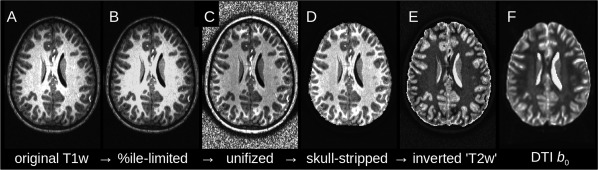
An example of the inversion of the IRCT method for generating a T2w‐like image from a T1w volume. The brightness values of the original volume (A) are ceilinged (B) based on the WB distribution. (C) WM and GM tissues are each intensity normalized to approximately uniform intensities. (D) The intracranial volume is extracted, and (E) the linear brightness inversion is performed. The resulting volume has similar relative tissue contrast to an acquired T2w volume, as well as to a standard DTI b ₀ (a similar slice is shown in panel F).

Figure A2.

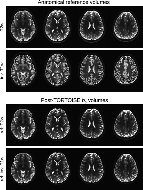
The T2w and inverse T1w data sets used as anatomical references in TORTOISE are shown in the top rows, respectively (axial slices, left = left). The bottom two rows show each of the average b ₀ volumes at the same locations after being processed by TORTOISE, and these volumes show a very high degree of similarity.

Figure A3.

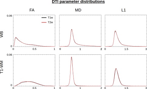
Normalized distributions of DTI parameters after TORTOISE processing are shown from across the WB (top row) and within the T1‐segmented WM (bottom row). The results of TORTOISE processing using the inverted T1w volume (red) and the standard T2w volume (black) are nearly identical. [Color figure can be viewed at http://wileyonlinelibrary.com]

Figure A4.

Axial slices (left = left) compare the overlap of WM masks derived from post‐TORTOISE DTI data, where FA > 0.2, for pipelines using either a standard T2w volume or an inverted T1w volume. The volumes show a high degree of overlap (red) across the cortex and much of the brain. Small differences (green and blue) are noticeable mainly within one voxel of the GM‐WM boundary, and in the most inferior slices, as well as in posterior regions. [Color figure can be viewed at http://wileyonlinelibrary.com]

Figure A5.

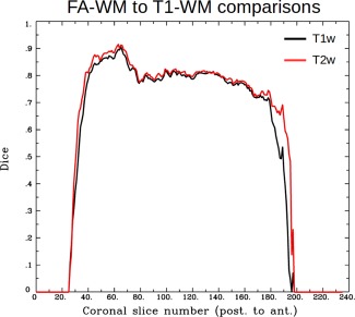
Dice coefficients showing the overlap in WM masks defined using DTI parameters (where FA > 0.2) and T1w segmentation. The Dice coefficient was calculated separately for each coronal slice in the aligned volumes, in order to show any local changes. The results of processing using TORTOISE and either a standard T2w volume (red) or an inverted T1w volume (black) are uniformly high and similar to each other across the brain, with the greatest difference apparent at the posterior‐most slices of the brain. [Color figure can be viewed at http://wileyonlinelibrary.com]

REFERENCES

- Aksoy M, Liu C, Moseley ME, Bammer R (2008): Single‐step nonlinear diffusion tensor estimation in the presence of microscopic and macroscopic motion. Magn Reson Med 59: 1138–1150. [DOI] [PMC free article] [PubMed] [Google Scholar]
- Alhamud A, Tisdall MD, Hess AT, Hasan KM, Meintjes EM, van der Kouwe AJW (2012): Volumetric navigators for real‐time motion correction in diffusion tensor imaging. Magn Reson Med 68:1097–1108. [DOI] [PMC free article] [PubMed] [Google Scholar]
- Alhamud A, Taylor PA, Laughton B, Hasan KM, van der Kouwe AJW, Meintjes EM (2015): Motion artifact reduction in pediatric diffusion tensor imaging using fast prospective correction. J Magn Reson Imaging 41:1353–1364. [DOI] [PMC free article] [PubMed] [Google Scholar]
- Alhamud A, Taylor PA, van der Kouwe AJW, Meintjes EM (2016): Real‐time measurement and correction of both B0 changes and subject motion in diffusion tensor imaging using a double volumetric navigated (DvNav) sequence. NeuroImage 1;126:60–71. [DOI] [PMC free article] [PubMed] [Google Scholar]
- Andersson JL, Skare S, Ashburner J (2003): How to correct susceptibility distortions in spin‐echo echo‐planar images: Application to diffusion tensor imaging. Neuroimage 20:870–888. [DOI] [PubMed] [Google Scholar]
- Ardekani S, Sinha U (2005): Geometric distortion correction of high‐resolution 3 T diffusion tensor brain images. Magn Reson Med 54:1163–1171. [DOI] [PubMed] [Google Scholar]
- Benner T, van der Kouwe AJW, Sorensen AG (2011): Diffusion imaging with prospective motion correction and reacquisition. Magn Reson Med 66:154–167. [DOI] [PMC free article] [PubMed] [Google Scholar]
- Cole JH, Farmer RE, Rees EM, Johnson HJ, Frost C, Scahill RI, Hobbs NZ (2014): Test‐retest reliability of diffusion tensor imaging in Huntington's disease. PLoS Curr 6: pii: ecurrents.hd.f19ef63fff962f5cd9c0e88f4844f43b. [DOI] [PMC free article] [PubMed] [Google Scholar]
- Cox RW (1996): AFNI: Software for analysis and visualization of functional magnetic resonance neuroimages. Comput Biomed Res 29:162–173. (1996): [DOI] [PubMed] [Google Scholar]
- Dice L (1945): Measures of the amount of ecologic association between species. Ecology 26:207–302. [Google Scholar]
- Dubois J, Kulikova S, Hertz‐Pannier L, Mangin JF, Dehaene‐Lambertz G, Poupon C (2014): Correction strategy for diffusion‐weighted images corrupted with motion: Application to the DTI evaluation of infants' white matter. Magn Reson Imaging 32:981–992. [DOI] [PubMed] [Google Scholar]
- Elhabian S, Gur Y, Vachet C, Piven J, Styner M, Leppert IR, Pike GB, Gerig G (2014): Subject‐motion correction in HARDI acquisitions: Choices and consequences. Front Neurol 5:240. [DOI] [PMC free article] [PubMed] [Google Scholar]
- Graham MS, Drobnjak I, Zhang H (2016): Realistic simulation of artefacts in diffusion MRI for validating post‐processing correction techniques. Neuroimage 125:1079–1094. [DOI] [PubMed] [Google Scholar]
- Heiervang E, Behrens TEJ, Mackay CE, Robson MD, Johansen‐Berg H (2006): Between session reproducibility and between subject variability of diffusion MR and tractography measures. Neuroimage 33:867–877. [DOI] [PubMed] [Google Scholar]
- Holdsworth SJ, Aksoy M, Newbould RD, Yeom K, Van AT, Ooi MB, Barnes PD, Bammer R, Skare S (2012): Diffusion tensor imaging (DTI) with retrospective motion correction for large‐scale pediatric imaging. J Magn Reson Imaging 36:961–971. [DOI] [PMC free article] [PubMed] [Google Scholar]
- Holland D, Kuperman JM, Dale AM (2010): Efficient correction of inhomogeneous static magnetic field‐induced distortion in echo planar imaging. Neuroimage 50:175–183. [DOI] [PMC free article] [PubMed] [Google Scholar]
- Irfanoglu MO, Walker L, Sarlls J, Marenco S, Pierpaoli C (2012): Effects of image distortions originating from susceptibility variations and concomitant fields on diffusion MRI tractography results. Neuroimage 61:275–288. [DOI] [PMC free article] [PubMed] [Google Scholar]
- Irfanoglu MO, Nayak A, Jenkins J, Hutchinson EB, Sadeghi N, Thomas CP, Pierpaoli C (2016): DR‐TAMAS: Diffeomorphic registration for tensor accurate alignment of anatomical structures. Neuroimage 132:439–454. [DOI] [PMC free article] [PubMed] [Google Scholar]
- Jenkinson M (1999): Measuring transformation error by RMS deviation. Tech. Rep. TR99MJ1, Oxford Center for Functional Magnetic Resonance Imaging of the Brain (FMRIB).
- Jezzard P, Barnett AS, Pierpaoli C (1998): Characterisation of and correction for eddy current artefacts in echo planar diffusion imaging. Magn Reson Med 39:801–812. [DOI] [PubMed] [Google Scholar]
- Kober T, Gruetter R, Krueger G (2012): Prospective and retrospective motion correction in diffusion magnetic resonance imaging of the human brain. NeuroImage 59:389–398. [DOI] [PubMed] [Google Scholar]
- Kong XZ, Zhen Z, Li X, Lu HH, Wang R, Liu L, He Y, Zang Y, Liu J (2014): Individual differences in impulsivity predict head motion during magnetic resonance imaging. PLoS One 22 9:e104989. [DOI] [PMC free article] [PubMed] [Google Scholar]
- Kreilkamp BA, Zacà D, Papinutto N, Jovicich J (2016): Retrospective head motion correction approaches for diffusion tensor imaging: Effects of preprocessing choices on biases and reproducibility of scalar diffusion metrics. J Magn Reson Imaging. 43:99–106. [DOI] [PubMed] [Google Scholar]
- Landman BA, Farrell JA, Jones CK, Smith SA, Prince JL, Mori S (2007): Effects of diffusion weighting schemes on the reproducibility of DTI‐derived fractional anisotropy, mean diffusivity, and principal eigenvector measurements at 1.5T. Neuroimage 36:1123–1138. [DOI] [PMC free article] [PubMed] [Google Scholar]
- Lazar M, Alexander AL (2003): An error analysis of white matter tractography methods: Synthetic diffusion tensor field simulations. Neuroimage 20:1140–1153. [DOI] [PubMed] [Google Scholar]
- Le Bihan D, Poupon C, Amadon A, Lethimonnier F (2006): Artifacts and pitfalls in diffusion MRI. J Magn Reson Imaging 24:478–488. [DOI] [PubMed] [Google Scholar]
- Leemans A, Jones DK (2009): The B‐matrix must be rotated when correcting for subject motion in DTI data. Magn Reson Med 61:1336–1349. [DOI] [PubMed] [Google Scholar]
- Ling J, Merideth F, Caprihan A, Pena A, Teshiba T, Mayer AR (2012): Head injury of head motion? Assessment and quantification of motion artifacts in diffusion tensor imaging studies. Hum Brain Mapp 33:50–62. (2012): [DOI] [PMC free article] [PubMed] [Google Scholar]
- Molfese PJ, Glen D, Mesite L, Pugh K, Cox RW (2015): The Haskins pediatric brain atlas. 21st Annual Meeting of the Organization for Human Brain Mapping (OHBM). p. 3511.
- Mukherjee P, Chung SW, Berman JI, Hess CP, Henry RG (2008): Diffusion tensor MR imaging and fiber tractography: Technical considerations. AJNR Am J Neuroradiol 2008;29:843–852. [DOI] [PMC free article] [PubMed] [Google Scholar]
- Norris DG (2001): Implications of bulk motion for diffusion‐weighted imaging experiments: Effects, mechanisms, and solutions. J Magn Reson Imaging 13:486–495. [DOI] [PubMed] [Google Scholar]
- Pierpaoli C, Walker L, Irfanoglu MO, Barnett A, Basser P, Chang L‐C, Koay C, Pajevic S, Rohde G, Sarlls J, Wu M (2010): TORTOISE: An Integrated Software Package for Processing of Diffusion MRI Data. ISMRM (2010) 18th Annual Meeting, Stockholm, Sweden, p 1597.
- Reese T, Heid O, Weisskoff R, Wedeen V (2003): Reduction of eddy‐current‐induced distortion in diffusion MRI using a twice‐refocused spin echo. Magn Reson Med 49:177–182. [DOI] [PubMed] [Google Scholar]
- Reuter M, Tisdall MD, Qureshi A, Buckner RL, van der Kouwe AJ, Fischl B (2015): Head motion during MRI acquisition reduces gray matter volume and thickness estimates. Neuroimage 107:107–115. [DOI] [PMC free article] [PubMed] [Google Scholar]
- Rohde GK, Barnett AS, Basser PJ, Marenco S, Pierpaoli C (2004): Comprehensive approach for correction of motion and distortion in diffusion‐weighted MRI. Magn Reson Med 51:103–114. [DOI] [PubMed] [Google Scholar]
- Smith S, Jenkinson M, Woolrich M, Beckmann C, Behrens T, Johansen‐Berg H, Bannister P, De Luca M, Drobnjak I, Flitney D, Niazy R, Saunders J, Vickers J, Zhang Y, De Stefano N, Brady J, Matthews P (2004): Advances in functional and structural MR image analysis and implementation as FSL. Neuroimage 23:208–219. [DOI] [PubMed] [Google Scholar]
- Taylor PA, Cho KH, Lin CP, Biswal BB (2012): Improving DTI tractography by including diagonal tract propagation. PLoS One 7:e43415. [DOI] [PMC free article] [PubMed] [Google Scholar]
- Taylor PA, Saad ZS (2013): FATCAT: (An efficient) functional and tractographic connectivity analysis toolbox. Brain Connect 3:523–525. [DOI] [PMC free article] [PubMed] [Google Scholar]
- Theys C, Wouters J, Ghesquière P (2014): Diffusion tensor imaging and resting‐state functional MRI‐scanning in 5‐ and 6‐year‐old children: Training protocol and motion assessment. PLoS One 9:e94019. [DOI] [PMC free article] [PubMed] [Google Scholar]
- Tijssen RH, Jansen JF, Backes WH (2009): Assessing and minimizing the effects of noise and motion in clinical DTI at 3 T. Hum Brain Mapp 30:2641–2655. [DOI] [PMC free article] [PubMed] [Google Scholar]
- Tisdall M, Hess AT, van der Kouwe AJ (2009): MPRAGE using EPI navigators for prospective motion correction. Proc Int Soc Magn Reson Med 29:4656. [Google Scholar]
- van der Kouwe AJW, Benner T, Salat DH, Fischl B (2008): Brain morphometry with multiecho MPRAGE. Neuroimage 40:559–569. [DOI] [PMC free article] [PubMed] [Google Scholar]
- Walker L, Chang L‐C, Koay CG, Sharma N, Cohen L, Ragini V, Pierpaoli C (2011): Effects of physiological noise in population analysis of diffusion tensor MRI data. NeuroImage 54:1168–1177. [DOI] [PMC free article] [PubMed] [Google Scholar]
- Wu M, Chang LC, Walker L, Lemaitre H, Barnett AS, Marenco S, Pierpaoli C (2008): Comparison of EPI distortion correction methods in diffusion tensor MRI using a novel framework. MICCAI 11:321–329. [DOI] [PMC free article] [PubMed] [Google Scholar]
Associated Data
This section collects any data citations, data availability statements, or supplementary materials included in this article.
Supplementary Materials