Common Statistical Pitfalls in Basic Science Research

Introduction

The analysis of clinical samples, population samples, and controlled trials is typically subjected to rigorous statistical review. This fact is understandable, given that the results of clinical investigation will often be used to inform patient care or clinical decision making. One would not want to predicate patient advice on research findings that are not correctly interpreted or valid. For this reason, most major journals publishing clinical research include statistical reviews as a standard component of manuscript evaluation for publication. Clinical data, regardless of publication venue, are often subject to rather uniform principles of review.

In contrast, basic science studies are often handled less uniformly, perhaps because of the unique challenges inherent in this type of investigation. A single basic science manuscript, for example, can span several scientific disciplines and involve biochemistry, cell culture, model animal systems, and even selected clinical samples. Such a manuscript structure is a challenge for analysis and statistical review. Not all journals publishing basic science articles use statistical consultation, although it is becoming increasingly common.1 In addition, most statistical reviewers are more comfortable with clinical study design than with basic science research. Consequently, there are multiple reasons why the statistical analysis of basic science research might be suboptimal. In this review, we focused on common sources of confusion and errors in the analysis and interpretation of basic science studies. The issues addressed are seen repeatedly in the authors' editorial experience, and we hope this article will serve as a guide for those who may submit their basic science studies to journals that publish both clinical and basic science research. We have discussed issues related to sample size and power, study design, data analysis, and presentation of results (more details are provided by Katz2 and Rosner3). We then illustrated these issues using a set of examples from basic science research studies.

Sample Size Considerations

Sample Size: What Constitutes the Experimental “n” in Basic Research?

The unit of analysis is the entity from which measurements of “n” are taken. The units could be animals, organs, cells, or experimental mixtures (eg, enzyme assays, decay curves). The sample size, which affects the appropriate statistical approach used for formal testing, is the number (ie, n value) of independent observations under 1 experimental condition. Most common statistical methods assume that each unit of analysis is an independent measurement. A common pitfall in basic science research is the treatment of repeated measurements of a unit of analysis as independent when, in fact, they are correlated, thus artificially increasing the sample size. A simple example is a single measurement (eg, weight) performed on 5 mice under the same condition (eg, before dietary manipulation), for n=5. If we measure the weight 12 times in 1 day, we have 12 measurements per mouse but still only 5 mice; therefore, we would still have n=5 but with 12 repeated measures rather than an n value of 5×12=60. In contrast, the 12 repeated measures of weight could be used to assess the accuracy of the mouse weights; therefore, the 12 replicates could be averaged to produce n=1 weight for each mouse. Things become even more vague when using cell culture or assay mixtures, and researchers are not always consistent. By convention, an independent experiment infers that the researcher has independently set up identical experiments each time rather than just measuring the outcome multiple times. The former reflects the inherent biological variability, whereas the latter may simply measure assay variability.

Sample Size Determination and Power

Sample size determination is critical for every study design, whether animal studies, clinical trials, or longitudinal cohort studies. Ethical considerations elevate the need for sample size determination as a formal component of all research investigations. In basic science research, studies are often designed with limited consideration of appropriate sample size. Sample sizes are often quite small and are not likely to support formal statistical testing of the underlying hypothesis. Although determining an appropriate sample size for basic science research might be more challenging than for clinical research, it is still important for planning, analysis, and ethical considerations. When determining the requisite number of experimental units, investigators should specify a primary outcome variable and whether the goal is hypothesis testing (eg, a statistical hypothesis test to produce an exact statistical significance level, called a P value) or estimation (eg, by use of a confidence interval). We find that most basic science studies involve hypothesis testing. In addition, investigators should specify the details of the design of the experiment to justify the choice of statistical test used. Will comparison groups, for example, be independent (eg, experimental units randomized to competing conditions) or dependent (the same units measured under each experimental condition, sometimes called a matched, paired, or repeated‐measures design)? Careful specification of the experimental design will greatly aid investigators in calculating sample size.

A particular challenge in sample size determination is estimating the variability of the outcome, particularly because different experimental designs require distinct approaches. With an independent samples design, for example, variability pertains to the outcome measure (eg, weight, vascular function, extent of atherosclerosis), whereas a paired samples design requires estimating the difference in the outcome measure between conditions over time. A common mistake is not considering the specific requirements to analyze matched or paired data. When hypothesis testing is to be performed, a sample size that results in reasonable power (ie, the probability of detecting an effect or difference if one exists) should be used. A typical “reasonable” value is ≥80% power. In basic science research, there is often no prior study, or great uncertainty exists regarding the expected variability of the outcome measure, making sample size calculations a challenge. In such cases, we recommend that investigators consider a range of possible values from which to choose the sample size most likely to ensure the threshold of at least 80% power.

An important implication of appropriate sample determination is minimizing known types of statistical errors. A significant statistical finding (eg, P<0.05 when the significance criterion is set at 5%) is due to a true effect or a difference or to a type I error. A type I error is also known as a false‐positive result and occurs when the null hypothesis is rejected, leading the investigator to conclude that there is an effect when there is actually none. The probability of type I error is equal to the significance criterion used (5% in this example). Investigators can limit type I error by making conservative estimates such that sample sizes support even more stringent significance criteria (eg, 1%). Conversely, a comparison that fails to reach statistical significance is caused by either no true effect or a type II error. A type II error is described as a false‐negative result and occurs when the test fails to detect an effect that actually exists. The probability of type II error is related to sample size and is most often described in terms of statistical power (power=1‐type II error probability) as the probability of rejecting a false‐null hypothesis. Minimizing type II error and increasing statistical power are generally achieved with appropriately large sample sizes (calculated based on expected variability). A common pitfall in basic science studies is a sample size that is too small to robustly detect or exclude meaningful effects, thereby compromising study conclusions.

Basic science studies often involve several outcome variables from the same sample (eg, group of mice), making sample size decisions challenging. In this instance, an efficient approach is to perform sample size computations for each outcome, and the largest practical sample size could be used for the entire experiment. If the calculated sample size is not practical, alternative outcome measures with reduced variability could be used to reduce sample size requirements.

Issues to Consider in Designing Studies

In designing even basic science experiments, investigators must pay careful attention to control groups (conditions), randomization, blinding, and replication. The goal is to ensure that bias (systematic errors introduced in the conduct, analysis, or interpretation of study results) and confounding (distortions of effect caused by other factors) are minimized to produce valid estimates of effect. Concurrent control groups are preferred over historical controls, and littermates make the best controls for genetically altered mice. With large samples, randomization ensures that any unintentional bias and confounding are equally present in control and experimental groups. In developing competing treatments or experimental conditions, the various conditions should be identical in every way except for the experimental condition under study. This includes control of conditions that may unknowingly have an impact on the effects of the treatments under study (eg, time of day, temperature). Ideally, investigators performing measurements should be blinded to treatment assignments and experimental conditions. Stratification is a means to combat bias and confounding. This technique provides for randomization of treatment and control groups equally across potential sources of bias and confounding, such as time of day; stratification by morning or afternoon time slots would prevent any impact by time of day. Replication is also a critical element of many experiments. Replication provides additional information to estimate desired effects and, perhaps more important, to quantify uncertainty in observed estimates (as outlined). The value of replication is understood; however, replication is useful only if the repeated experiment is conducted under the same experimental conditions.

Investigators can also minimize variability by carefully planning how many treatments, experimental conditions, or factors can be measured in an individual unit (eg, animal). One might wish to determine, for example, the impact of genotype and diet on animal weight, blood pressure, left ventricular mass, and serum biomarkers. It is common to see investigators design separate experiments to evaluate the effects of each condition separately. This may not be the most efficient approach and introduces additional bias and confounding by performing serial sets of experiments that are separated in time. In contrast, factorial experiments, in which multiple conditions or factors are evaluated simultaneously, are more efficient because more information can be gathered from the same resources. In the above example, wild‐type and genetically altered littermates could be randomized in sufficient numbers to competing diets and observed for blood pressure, left ventricular mass, and serum biomarkers. This design provides information on the effect of diet, the effect of genotype, and the combination of the 2. It might be that the effect of diet and genotype is additive, or there may be a statistical interaction (a different effect of diet on blood pressure depending on genotype). This latter observation would escape detection if performed in separate experiments, and the factorial design has the advantage of involving fewer mice than would be required for the 2 separate experiments.

Issues in Presenting Data

A critically important first step in any data analysis is a careful description of the data. This description includes the sample size (experimental n value) and appropriate numerical and graphical summaries of the data. The sample size is most informative and is presented to provide the reader with the true size of the experiment and its precision. The habit of presenting sample sizes as ranges (eg, n=5 to 12 in each group) is not useful from a statistical perspective. It is more appropriate to clearly indicate the exact sample size in each comparison group.

In clinical studies, the first summary often includes descriptive statistics of demographic and clinical variables that describe the participant sample. Continuous variables such as age, weight, and systolic blood pressure are generally summarized with means and standard deviations. If variables are not normally distributed or are subject to extreme values (eg, cholesterol or triglyceride levels), then medians and interquartile ranges (calculated as Q₃−Q₁, in which Q indicates quartile) are more appropriate. Several approaches can be used to determine whether a variable is subject to extreme or outlying values. One of the most popular is based on Tukey fences, which represent lower and upper limits defined by the upper and lower quartiles and the interquartile range, specifically, values below Q₁−1.5 (Q₃−Q₁) or above Q₃+1.5 (Q₃−Q₁).4 Extreme values should always be examined carefully for errors and corrected if needed but never removed.

In basic science studies, investigators often move immediately into comparisons among groups. If the outcome being compared among groups is continuous, then means and standard errors should be presented for each group. There is often confusion about when to present the standard deviation or the standard error. Standard deviations describe variability in a measure among experimental units (eg, among participants in a clinical sample), whereas standard errors represent variability in estimates (eg, means or proportions estimated for each comparison group). When summarizing continuous outcomes in each comparison group, means and standard errors should be used. When summarizing binary (eg, yes/no), categorical (eg, unordered), and ordinal (eg, ordered, as in grade 1, 2, 3, or 4) outcomes, frequencies and relative frequencies are useful numerical summaries; when there are relatively few distinct response options, tabulations are preferred over graphical displays (Table 1).

Table 1.

Summarizing Outcomes in Clinical and Basic Science Studies

Outcome Variable	Statistics
Goal: Describe the distribution of observations measured in the study sample
Continuous	Sample size (n) and Mean and SD ora Median (Q2) and interquartile range (Q3−Q1)
Binary, categorical, or ordinal	Sample size (n) and relative frequency (%)
Goal: Compare groups
Continuous	Means and SEs for each group
Binary, categorical, or ordinal	Proportions (%) and SEs for each group

Q indicates quartile.

^aMean and SD if there are no extreme or outlying values.

Graphical Comparisons

Several options exist for investigators to informatively display data in graphical format. In some experiments, it might be useful to display the actual observed measurements under each condition. If the sample size is relatively small (eg, n<20), then dot plots of the observed measurements are very useful (Figure 1). With larger samples, however, summary measures are needed. For continuous outcomes, means and standard errors should be provided for each condition (Figure 2). Trend lines should be included in displays to highlight trends over time when data are measured repeatedly in the same experimental unit, and again, measures of variability should be included in these displays (Figure 3). Ordinal and categorical variables are best displayed with relative frequency histograms and bar charts, respectively (Figure 4).

Figure 1.

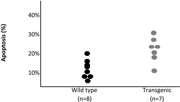
Dot plot of percentage of apoptosis by type.

Figure 2.

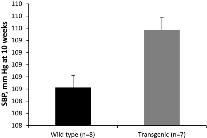
Mean and standard error of systolic blood pressure (SBP) by type.

Figure 3.

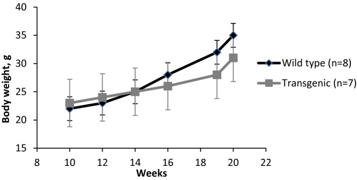
Changes in body weight over time by type.

Figure 4.

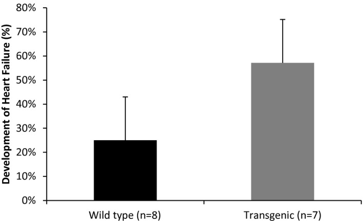
Development of heart failure (%) by type.

Statistical Analyses

Appropriate statistical tests depend on the study design, the research question, the sample size, and the nature of the outcome variable. These issues and their implications are discussed next.

Independent versus repeated measurements

An important consideration in determining the appropriate statistical test is the relationship, if any, among the experimental units in the comparison groups. One must understand if the experimental units assigned to comparison groups are independent (eg, only 1 treatment per unit) or repeated measurements taken on the same set of experimental units under differing conditions. This distinction is very important because the former requires analytic methods for independent samples and the latter involves methods that account for correlation of repeated measurements. It is common to find basic science studies that neglect this distinction, often to the detriment of the investigation because a repeated‐measures design is a very good way to account for innate biological variability between experimental units and often is more likely to detect treatment differences than analysis of independent events.

Parametric versus nonparametric data

It is also important to note that appropriate use of specific statistical tests depends on assumptions or assumed characteristics about the data. Failure to satisfy these assumed characteristics can lead to incorrect inferences and is a common oversight in basic science studies. Suppose we have a study involving 1 experimental factor with 3 experimental conditions (eg, low, moderate, and high dose) and a control. Outcomes observed under each of the 4 conditions could be represented by means (for continuous variables) or proportions (for binary variables) and typically would be compared statistically with ANOVA or a chi‐square test, respectively. Each of these statistical tests assumes specific characteristics about the data for their appropriate use. The basic assumptions for ANOVA are independence (ie, independent experimental units and not repeated assessments of the same unit), normally distributed outcomes, and homogeneity of variances across comparison groups. With large samples (n>30 per group), normality is typically ensured by the central limit theorem; however, with small sample sizes in many basic science experiments, normality must be specifically examined. This can be done with graphic displays or assessment of distributional properties of the outcome within the current study or reported elsewhere (note that the assumption of normality relates to normality of the outcome in the population and not in the current study sample alone). There are also specific statistical tests of normality (eg, Kolmogorov‐Smirnov, Shapiro‐Wilk), but investigators should be aware that these tests are generally designed for large sample sizes.5 If one cannot assume normality, the most conservative strategy is to use a nonparametric test designed for nonnormal data. Another alternative is to transform the data (by log or square root) to yield a normal distribution and then to perform analyses on the transformed data. The chi‐square test (used with categorical and ordinal outcomes) also assumes independence and an expected count of at least 5 in each comparison group. If the latter condition is not satisfied, an alternative exact test (eg, Fisher's exact test) should be used. Table 2 outlines some common statistical procedures used for different kinds of outcomes (eg, continuous, categorical) to make comparisons among competing experimental conditions with varying assumptions and alternatives.

Table 2.

Examples of Statistical Tests for Specific Applications

Outcome Variable	Number of Experimental Groups for Factor	Group Structure	Assumptions for Parametric Test	Parametric Test Assumptions Met	Nonparametric or Exact Test Assumptions Not Met
Continuous	2	Independent	Independence of observations, normality or large samples, and homogeneity of variances	Unpaired t test	Mann–Whitney U or Wilcoxon rank sum test
		Dependent (matched)	Independence of pairs, normality or large samples, and homogeneity of variances	Paired t test	Wilcoxon signed rank test
	>2	Independent	Independence of observations, normality or large samples, and homogeneity of variances	ANOVA	Kruskal–Wallis test
		Dependent (matched)	Repeated measures in independent observations, normality or large samples, and homogeneity of variances	Repeated‐measures ANOVA	Freidman test
Binary, categorical, or ordinal	≥2	Independent	Independence of observations, expected count >5 in each cell	Chi‐square test	Fisher's exact test
		Dependent (matched)	Independence of pairs	McNemar test

In many settings, multiple statistical approaches are appropriate. The examples given are general guidelines.

Multiple experimental factors

When the effects of >1 experimental condition are of interest, higher order or factorial ANOVA may be appropriate. These designs allow investigators to test for effects of each experimental condition alone (main effects) and to test whether there is a statistical interaction (difference in the effect of 1 factor as a function of another) on the outcome of interest. To perform factorial ANOVA, one needs to follow a specific order of analysis to arrive at valid findings. An overall test is performed first to assess whether differences are present among the responses defined by the factors of interest. If such a finding is significant, a test is then run for statistical interaction. In the absence of statistical interaction, one is free to test for the main effects of each factor. If the statistical interaction is significant, then the interaction should be reported and formal tests for main effects should be omitted (because there are different associations depending on the second factor, as discussed in detail by Kleinbaum et al6).

Note that 1‐factor and higher order ANOVAs are also based on assumptions that must be met for their appropriate use (eg, normality or large samples). ANOVA is robust for deviations from normality when the sample sizes are small but equal. Investigators should try to design studies with equal numbers in each comparison group to promote the robustness of statistical tests.

Repeated measurements

Some experiments may involve a combination of independent and repeated factors that are also sometimes called between and within factors, respectively. Consider a study with 3 different experimental groups (eg, animal genotypes) with outcomes measured at 4 different time points. An appropriate analytic technique is a repeated‐measures ANOVA with 1 between factor (ie, genotype) and 1 within factor (ie, time). This type of analysis accounts for the dependencies of observations measured repeatedly. Investigators often design careful studies with repeated measurements over time, only to ignore the repeated nature of the data with analyses performed at each time point. Such an approach not only fails to examine longitudinal effects contained in the data but also results in decreased statistical power compared with a repeated‐measures analysis.

Multiple testing

Basic science experiments often have many statistical comparisons of interest. Each time a statistical test is performed, it is possible that the statistical test will be significant by chance alone when, in fact, there is no effect (ie, a type I error). Foremost, only those statistical comparisons that are of scientific interest should be conducted. Because each test carries a nonzero probability of incorrectly claiming significance (ie, a finite false‐positive rate), performing more tests only increases this potential error. Multiple comparison procedures are techniques that allow for more comparisons but that control the overall type I error rate for the set of all comparisons. Pairwise comparisons (2 at a time) are perhaps the most popular, but general contrasts (eg, comparing the mean of groups 1 and 2 with the mean of groups 3 and 4) are also possible with these procedures. Many multiple comparison procedures exist, and most are available in standard statistical computing packages. The procedures differ in terms of how they control the overall type I error rate; some are more suitable than others in specific research scenarios.7, 8 If the goal is to compare each of several experimental conditions with a control, the Dunnett test is best. If it is of interest to compare all pairs of experimental conditions, then the Tukey or Duncan test may be best, depending on the number of desired comparisons and the sample sizes. The Bonferroni adjustment is another popular approach with which the significance criterion (usually α=0.05) is set at α/k, in which k represents the number of comparisons of interest. Although this approach is very easy to implement, it is overly conservative. Investigators should evaluate the various procedures available and choose the one that best fits the goals of their study. Because many basic science experiments are exploratory and not confirmatory, investigators may want to conduct more statistical tests without the penalty of strict control for multiple testing. This approach can be appropriate, but with many statistical tests, investigators must recognize the possibility of a false‐positive result and, at a minimum, recognize this particular limitation.

Analyzing survival

In some experiments, the outcome of interest is survival or time to an event. Time‐to‐event data have their own special features and need specialized statistical approaches to describe and compare groups in terms of their survival probabilities. A key feature of survival data is censoring, which occurs when some experimental units do not experience the event of interest (eg, development of disease, death) during the observation period. Investigators might observe mice for 12 weeks, during which time some die and others do not; for those that do not, the investigators record 12 weeks as the last time these mice were observed alive. This value is a censored time and is less than the time to event, which will occur later (and is unmeasured). Because of censoring, standard statistical techniques (eg, t tests or linear regression) cannot be used. Survival data are efficiently summarized with estimates of survival curves, and the Kaplan–Meier approach is well accepted. If a Kaplan–Meier curve is displayed in a figure, it is important to include the number of units at risk over time along with estimates of variability (eg, confidence limits along with estimates of survival probabilities over time). Comparisons between experimental conditions in terms of survival are often performed with the log‐rank test. The log‐rank test is a popular nonparametric test and assumes proportional hazards (described in more detail by Rao and Schoenfeld9). Survival analyses can be particularly challenging for investigators in basic science research because small samples may not result in sufficient numbers of events (eg, deaths) to perform meaningful analysis. Investigators should always perform sample size computations, particularly for experiments in which mortality is the outcome of interest, to ensure that sufficient numbers of experimental units are considered to produce meaningful results.

Recognizing limitations

In every study, it is important to recognize limitations. In basic science research, investigators often have small sample sizes, and some of their statistical comparisons may fail to reach statistical significance. It is important to recognize that the lack of significance may be due to low statistical power. In such a case, the observed effects can be used to design a larger study with greater power. In basic science research, confounding due to other factors might be an issue; carefully designed experiments can minimize confounding. If there is potential for other factors to influence associations, investigators should try to control these factors by design (eg, stratification) or be sure to measure them so that they might be controlled statistically using multivariable models, if the sample size allows for such models to be estimated.

Hypothetical Examples

Example 1

We wish to compare organ blood flow recovery at 7 days after arterial occlusion in 2 different strains of mice. The outcome of interest is normalized blood flow (a continuous outcome), and the comparison of interest is mean normalized blood flow between strains. A single measurement is taken for each mouse. In this example, the unit of analysis is the mouse, and the sample size is based on the number of mice per strain. Data can be summarized as shown in Table 3 and compared statistically using the unpaired t test (assuming that normalized blood flow is approximately normally distributed). If the outcome were not approximately normally distributed, then a nonparametric alternative such as the Wilcoxon rank sum or Mann–Whitney U test could be used instead.

Table 3.

Normalized Blood Flow by Strain

Strain	Sample Size	Normalized Blood Flow, Mean (SE)	P Valuea
1	8	0.65 (0.50)	0.58
2	10	0.29 (0.40)

^aUnpaired t test.

Example 2

We wish to compare organ blood flow recovery over time after arterial occlusion in 2 different strains of mice. The outcome of interest is again normalized blood flow (a continuous outcome), and the comparison of interest is the trajectory (pattern over time) of mean normalized blood flow between strains. The unit of analysis is the mouse, and we have repeated measurements of blood flow (before occlusion, at the time of occlusion [time 0], and then at 1, 3, 7, 14, 21, and 28 days). Data can be summarized as shown in Figure 5, in which means and standard error bars are shown for each time point and compared statistically using repeated‐measures ANOVA (again, assuming that normalized blood flow is approximately normally distributed). Note that analyses at each time point would not have addressed the main study question and would have resulted in a loss of statistical power.

Figure 5.

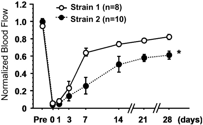
Blood flow over time by strain. *P<0.05.

Example 3

We wish to compare apoptosis in cell isolates in 3 different strains of mice (wild type and 2 strains of transgenic [TG] mice) treated with control (Ad‐LacZ) versus adenoviruses expressing catalase or superoxide dismutase. The outcome of interest is percentage of apoptosis (a continuous outcome), and the comparison of interest is percentage of apoptosis among strains. Six isolates were taken from each strain of mice and plated into cell culture dishes, grown to confluence, and then treated as indicated on 6 different occasions. The unit of analysis is the isolate, and data are combined from each experiment (different days) and summarized as shown in Figure 6. The data are means and standard errors taken over n=6 isolates for each type of mouse and condition.

Figure 6.

Percentage of apoptosis by strain. *P<0.05 against wild type treated with Ad‐LacZ. †P<0.05 between treated TG1 mice and TG1 treated with Ad‐LacZ. ‡P<0.05 between treated TG2 mice and TG2 treated with Ad‐LacZ. Cat indicates catalase; SOD, superoxide dismutase; TG, transgenic; WT, wild type.

Several statistical comparisons are of interest. Mean percentage of apoptosis can be compared among strains treated with control (Ad‐LacZ) using t tests comparing 2 groups or ANOVA comparing >2 groups, assuming that the percentage of apoptosis is approximately normally distributed (significant differences [P<0.05] are noted against wild type treated with Ad‐LacZ). Similar tests can be conducted for TG mice (significant differences [P<0.05] are noted between treated TG1 mice and TG1 treated with Ad‐LacZ and between treated TG2 mice and TG2 treated with Ad‐LacZ).

Example 4

We wish to compare cell protein as an index of cell growth in fibroblasts from 2 different strains of mice (wild type and TG) after fibroblasts are plated and allowed to grow for 0, 1, 3, 5, 7, and 9 hours. At the indicated time, cells are examined under a microscope, and cell protein is determined in the well using a calibrated grid. The analysis involves 7 different isolates of cells. The outcome of interest is cell protein (a continuous outcome), and the comparison of interest is the change in cell protein over time between strains. Again, multiple mice are used to grow a large number of cells that are then frozen in aliquots. On 7 different occasions, the cells are thawed and grown into the plates, and the experiments are performed. The unit of analysis is the isolate, and we have repeated measurements of cell protein at baseline (time 0) and then at 1, 3, 5, 7, and 9 hours. Data can be summarized as shown in Figure 7 and are displayed as means and standard error bars for each time point and compared statistically using repeated‐measures ANOVA (again, assuming that cell protein levels are approximately normally distributed).

Figure 7.

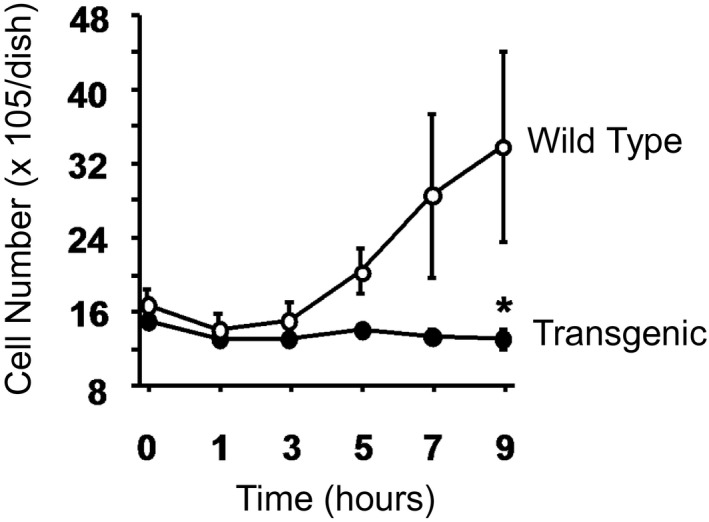
Cell protein over time by strain. *P<0.05.

Conclusions

Basic science studies are complex because they often span several scientific disciplines. Summarizing evidence and drawing conclusions based on the data are particularly challenging because of the complexity of study designs, small sample sizes, and novel outcome measures. Careful attention to the research question, outcomes of interest, relevant comparisons (experimental condition versus an appropriate control), and unit of analysis (to determine sample size) is critical for determining appropriate statistical tests to support precise inferences. Investigators must carefully evaluate assumptions of popular statistical tests to ensure that the tests used best match the data being analyzed. Figure 8 walks investigators through a series of questions that lead to appropriate statistical techniques and tests based on the nature of the outcome variable, the number of comparison groups, the structure of those groups, and whether or not certain assumptions are met. Many statistical tests are robust, meaning that they work well not only when assumptions are met but also when there are mild departures from assumptions. Investigators must be aware of assumptions and design studies to minimize such departures.

Figure 8.

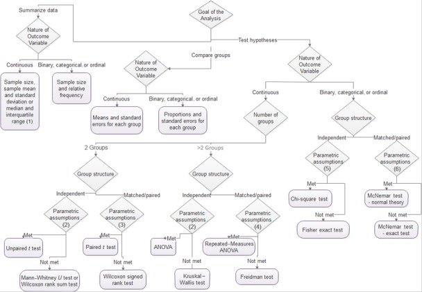
Determining what statistical technique or test to do when: (1) mean and standard deviation if no extreme or outlying values are present; (2) independence of observations, normality or large samples, and homogeneity of variances; (3) independence of pairs, normality or large samples, and homogeneity of variances; (4) repeated measures in independent observations, normality or large samples, and homogeneity of variances; (5) independence of observations and expected count >5 in each cell; (6) repeated measures in independent observations.

Disclosures

None.

J Am Heart Assoc. 2016;5:e004142 doi: 10.1161/JAHA.116.004142.

References

- 1. McNutt M. Raising the bar. Science. 2014;345:9. [DOI] [PubMed] [Google Scholar]
- 2. Katz M. Study Design and Statistical Analysis: A Practical Guide for Clinicians. New York, NY: Cambridge University Press; 2006. [Google Scholar]
- 3. Rosner B. Fundamentals of Biostatistics. 7th ed Boston, MA: Brooks/Cole ‐ Cengage Learning; 2010. [Google Scholar]
- 4. Hoaglin DC, John W. Tukey and data analysis. Stat Sci. 2003;18:311–318. [Google Scholar]
- 5. Ghasemi A, Zahediasl S. Normality tests for statistical analysis: a guide for non‐statisticians. Int J Endocrinol Metab. 2012;10:486–489. [DOI] [PMC free article] [PubMed] [Google Scholar]
- 6. Kleinbaum DG, Kupper LL, Muller KE. Applied Regression Analysis and Other Multivariable Methods. 2nd ed Boston, MA: PWS‐Kent Publishing Company; 1988. [Google Scholar]
- 7. D'Agostino RB, Massaro J, Kwan H, Cabral H. Strategies for dealing with multiple treatment comparisons in confirmatory clinical trials. Drug Inf J. 1993;27:625–641. [Google Scholar]
- 8. Cabral HJ. Statistical primer for cardiovascular research: multiple comparisons procedures. Circulation. 2008;117:698–701. [DOI] [PubMed] [Google Scholar]
- 9. Rao SW, Schoenfled DA. Statistical primer for cardiovascular research: survival methods. Circulation. 2007;115:109–113. [DOI] [PubMed] [Google Scholar]