Fluctuation of similarity (FLUS) to detect transitions between distinct dynamical regimes in short time series

Abstract

A method to identify distinct dynamical regimes and transitions between those regimes in a short univariate time series was recently introduced [1], employing the computation of fluctuations in a measure of nonlinear similarity based on local recurrence properties. In the present work, we describe the details of the analytical relationships between this newly introduced measure and the well known concepts of attractor dimensions and Lyapunov exponents. We show that the new measure has linear dependence on the effective dimension of the attractor and it measures the variations in the sum of the Lyapunov spectrum. To illustrate the practical usefulness of the method, we identify various types of dynamical transitions in different nonlinear models. We present testbed examples for the new method’s robustness against noise and missing values in the time series. We also use this method to analyze time series of social dynamics, specifically an analysis of the U.S. crime record time series from 1975 to 1993. Using this method, we find that dynamical complexity in robberies was influenced by the unemployment rate until the late 1980’s. We have also observed a dynamical transition in homicide and robbery rates in the late 1980’s and early 1990’s, leading to increase in the dynamical complexity of these rates.

I. INTRODUCTION

One of the central challenges in nonlinear time series analysis has been to develop methodologies to identify and predict dynamical transitions, i.e., time points where the dynamics show a qualitative change [1–12]. The application of such methods is widespread in a variety of areas of science and society [13]. For example, such approaches could be useful in medicine in identifying pathological activities of vital organs such as the heart and the brain from ECG and EEG data [14–16]. In earth sciences, one can use these methods to identify tipping points in modern and paleoclimate data sets [2, 7, 9–11, 17]. In the analysis of financial data, these methods may be used to better comprehend the behavior of markets and their vulnerabilities [18–20]. In physics, one may similarly study the response of an interacting many-body system to an external perturbation [21]. Finally, such methods could be used to analyze social and economic indictors to better understand societal changes and to predict possible future changes [13, 18–20].

The challenge in developing such methods is that there may be a variety of reasons in a particular system that can lead to different types of qualitative changes in the dynamics [3–5, 22–24]. Common reasons might include the evolving control parameters of the system passing through a bifurcation point, the rate of change of these control parameters, internal feedbacks, and noise induced effects [3–5, 22, 24]. In many natural systems it has been suggested that dynamic bifurcations lead to critical transitions in their dynamical state [24–26]. While these transitions are visually apparent and can be identified with little effort in some cases, in other cases these transitions may be much more subtle, especially where transition occurs from one chaotic regime to another complex chaotic regime. For example, in palaeoclimate studies, Dansgaard-Oeschger events on millennial time scales are visible in ice records to the naked eye and have been hypothesised to be caused by a noise induced transition [27–29]. In contrast, on similar time scales we do not observe such visibly apparent transitions in many other components of climate, such as the Indian summer monsoon, though it has also gone through dynamical transitions between distinct chaotic regimes due to variations of Milankovitch cycles [1, 30, 31], and we need more careful analysis. Similarly, certain brain states like sleep cycling or epileptic seizure are easily detectable from EEG data but gamma rhythms or the ultra-slow BOLD rhythms are harder to detect without more sophisticated mathematical tools to identify such dynamical transitions [32]. The intricacies and diversities involved in the origins of dynamical transitions make it difficult to develop one single method to identify and quantify all possible types of transitions. Rather, we need to have a toolbox consisting of several methodologies and approaches inspired by the paradigm of nonlinear dynamics to solve such problems. The case we will be most interested in here in the present work is where the changes in one single control parameter takes the system from a regime of one dynamical complexity to another dynamic state of different complexity. The method used here is particularly applicable when the available time series is relatively short (from several hundred to a few thousand time points).

Most of the widely used methods for the above mentioned applications are linear, such as auto correlation functions and detrended fluctuation analysis, among others [8, 11, 33–35]. But some methods for the analysis of time series using the paradigm of nonlinear dynamics have also shown tremendous promise, including recurrence plot based methodologies such as recurrence quantification analysis and recurrence network analysis [2, 7, 9, 10, 36–41]. The method discussed here—which we call FLUS (FLUctuation of Similarity)—is based on the concept of nonlinear similarity between two time points. FLUS is computationally simple, automatized, and yet extremely robust in distinguishing distinct dynamical regimes and identifying time points where transitions occur between these distinct dynamical regimes, even in the case where available time series is short. FLUS also tends to work well in the presence of noise and missing values.

FLUS was previously briefly introduced in the context of analyzing a short paleoclimatic time series of the Indian summer monsoon [1]. In the present manuscript, we for the first time present the method in full theoretical detail. In particular, we discuss in detail the analytical properties of the newly introduced measure and relate them to more standard concepts in nonlinear time series analysis such as attractor dimensions and Lyapunov exponents, providing a deeper understanding of the measure and its properties as well as its possible limitations. We also present an extensive numerical testing of this method, not previously provided in [1], using a variety of nonlinear dynamical models to demonstrate the capabilities of the method in distinguishing different dynamical regimes and in identifying transitions between them. We also include tests of the method’s robustness in the presence of observational noise and missing values, which are among the common problems encountered in time series analysis. Finally, we also present a novel example application of the method, analyzing crime rate time series from the U.S.

This paper is organized as follows. In Sec. II, we describe the method and some of the analytical results about it, with supporting numerical results. In Sec. III, we illustrate the strengths and practical utility of this method using several different numerical cases of dynamical transitions in nonlinear systems. We also test the method’s robustness against the presence of noise and missing values in a pragmatic nonlinear model. In Sec. IV, we apply the method to the question of the role of unemployment in robberies and homicides by considering the corresponding time series in the U.S. from 1975 to 1993.

II. FLUCTUATION OF SIMILARITY (FLUS)

Let x_j represent the jth vector of a delay embedded time series of length N. The embedding dimension m and time delay L are estimated respectively by false nearest neighbors and mutual information, as often done in nonlinear time series analysis [3–5, 42, 43]. In this reconstructed phase space, we denote the neighborhood containing k nearest neighbors of any point x_j by U(x_j) = {x_l : ∥x_j – x_l∥ < ϵ_j ∣ #(x_l) = k}, where the set l contains indices of the k nearest neighbors and ∥ · ∥ is a specified norm. Because we choose a fixed number of k nearest neighbors for each point x_j, ϵ_j varies with the change in the values of k i.e., ϵ_j = ϵ_j(k). Throughout the present text, we express k as a percentage of the total number of points N and use Euclidean distance if not indicated otherwise. The pointwise closeness of x_j to its k neighbors is obtained as the mean distance

$$d\left({\mathrm{x}}_j\right)=\frac{1}{k}\sum _{l\in U\left({\mathrm{x}}_j\right)}\Vert {\mathrm{x}}_j-{\mathrm{x}}_l\Vert .$$ (1)

At a later time j + τ, the neighborhood of x_j+τ is generally different from that of x_j, so we calculate the closeness of x_j+τ to the neighborhood of x_j by means of a conditional distance, defined as

$$d\left({\mathrm{x}}_{j+\tau }\mid {\mathrm{x}}_j\right)=\frac{1}{k}\sum _{l\in U\left({\mathrm{x}}_j\right)}\Vert {\mathrm{x}}_{j+\tau }-{\mathrm{x}}_{l+\tau }\Vert .$$ (2)

The dynamical similarity of x_j conditioned to x_j+τ can then be defined by

$$S_{j\mid j+\tau }=\frac{d\left({\mathrm{x}}_j\right)}{d\left({\mathrm{x}}_{j+\tau }\mid {\mathrm{x}}_j\right)}.$$ (3)

Larger values of S_j∣j+τ indicate higher similarities in the signal (i.e., for a periodic trajectory with period T, x_j = x_j+nT yields a periodic variation of S_j∣j+τ). It is easy to see that S_j∣j+τ is time dependent and relies on the initial conditions. The distribution of inter-spike interval of S_j∣j+τ reflects the associated recurrent period information, which shows unique properties for different dynamics (i.e., quasiperiodic or chaotic [44]). Fully comparing two time points, S_j+τ∣j characterizing the similarity of x_j+τ conditioned to x_j can also be calculated, noting that S_j+τ∣j need not be the same as S_j∣j+τ since the neighborhoods used in the calculations of d(x_j+τ∣x_j) and d(x_j∣x_j+τ) can be different. A similar measure has been used previously to estimate the nonlinear interdependency in bivariate studies [45], where the conditional distance was calculated between time points coming from two separate time series.

The measure S_j∣j+τ, indicating local properties of the time series, is computationally cumbersome to calculate for all possible S_j∣j+τ for a complete time series. We therefore devise a strategy to obtain a measure from S_j∣j+τ which is not only computationally simpler but also depends on the global properties of the attractor and will thereby be sensitive to dynamical transitions. To achieve this task, we first need to discuss the kinds of behaviors that we would recognize as dynamical transitions. For these purposes, let us consider two consecutive time points in a deterministic system with a locally sufficiently smooth mapping ϕ such that

$${\mathrm{x}}_{j+1}=\phi \left({\mathrm{x}}_j\right).$$ (4)

We are particularly interested in the situations where these strong constraints on ϕ and its local behavior break down, indicating a dynamical transition. If we fix τ = 1 and if there is no dynamical transition between j and j + 1, then we expect (as explained in detail in the next section, and see also Fig. 1 for a schematic representation of the associated concepts) the values of a finite time series S_j∣j+1 to fluctuate around a constant value μ_S specific to the mapping ϕ. If a dynamical transition occurs between j and j + 1, we expect substantially larger fluctuations in S_j∣j+1. We therefore aim to quantify such differences in terms of the variance of S_j∣j+1 over a window of n points:

$${\sigma }_S^2=\langle {\left(S_{j\mid j+1}-{\mu }_S\right)}^2\rangle ,$$ (5)

where μ_S = ⟨S_j∣j+1⟩ and ⟨·⟩ denotes an average over n points. We call σ_S the fluctuation of similarity (FLUS). Our numerical experimentation with a variety of nonlinear models with different kinds of transitions demonstrates that σ_S is a robust measure for identifying distinct dynamical regimes and corresponding transitions. FLUS shows even more subtle transitions than the standard measure of Lyapunov exponents, and its potential has been previously demonstrated using chaotic transitions in the logistic map [1]. Here we analyze several other nonlinear models using FLUS, to further explore its properties and demonstrate its effectiveness.

FIG. 1.

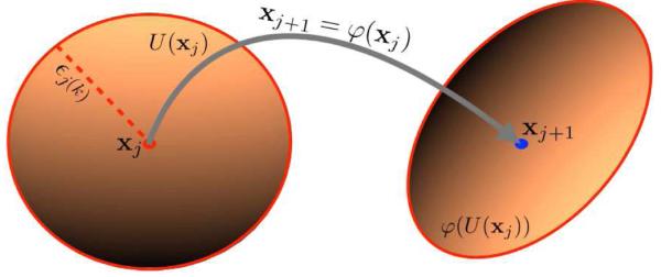
(Color online) Schematic representation of the ϵ_j(k) ball neighborhood U(x_j), corresponding to the k nearest neighbors of x_j, and its deformation (region within red boundary) due to application of the mapping ϕ, x_j+1 = ϕ(x_j). Note that the neighborhood of x_j+1 corresponding to its k nearest neighbors is usually different. Locally at x_j the mapping ϕ is approximated by a linear transformation. Expansion of U(x_j) by inclusion of more points rescales ϕ(U(x_j) by stretching or contraction in different directions. Hence, their radii will scale by the same exponent.

Before we employ σ_S to identify dynamical transitions and distinguish different dynamical regimes in a time series, first we must understand what are those analytical properties of σ_S that give it the capability to achieve these tasks. In the next subsection, we show that σ_S is linearly dependent on the effective dimension of the attractor in the absence of transitions. The concept of dimension of an attractor is inherently related to the complexity present in a time series originating from a nonlinear dynamical system [2–5]. Hence, showing an analytical relationship between σ_S and the effective dimension of the attractor amounts to demonstrating a dependence of σ_S on the dynamical complexity present in the time series. This relationship gives σ_S the capability of identifying changes in the dynamical regimes. In the process of exploring this relationship we also present some numerical arguments for σ_S working well in the case of short time series. We then discuss the relationship between the above introduced measures and the Lyapunov spectrum of the system, which is significant because the spectrum of Lyapunov exponents is perhaps the most widely used concept for measuring and understanding chaotic dynamics [3–5]. We will establish relationships between the similarity measure S_j∣j+1 and the Lyapunov spectrum, yielding insight into the features of σ_S and its possible applications for measuring or providing information about the Lyapunov exponents, which could in turn be used to classify system dynamics.

A. Relationship with attractor dimensions

FLUS relies on comparing dynamical similarity of two consecutive time points in the embedded space, in terms of calculations of S_j∣j+1 for the dynamics under study. To get further detailed insights into the properties of S_j∣j+1, we investigate the scalings of the mean distances d(x_j) and d(x_j+1∣x_j) with the number of nearest neighbors considered in defining the respective neighborhoods [45].

Suppose that a vector x_j in phase space has k nearest neighbors. Let $\overline{d}\left({\mathrm{x}}_j\right)$ be the mean density of the whole point cloud around x_j, i.e., $\overline{d}\left({\mathrm{x}}_j\right)=\frac{1}{N}{\sum }_{k=1}^N\Vert {\mathrm{x}}_j-{\mathrm{x}}_k\Vert$. For k ≪ N, we expect the following scaling law (see [45–50] for analytical details):

$$\frac{d\left({\mathrm{x}}_j\right)}{\overline{d}\left({\mathrm{x}}_j\right)}\approx a_j{\left(k∕N\right)}^{{\alpha }_j},$$ (6)

where N is the length of the time series and a_j is a scaling coefficient. In the N → ∞ limit, α_j = D_F, where 1/D_F is the effective dimension of the attractor. First introduced in [46], 1/D_F has been conjectured in [49, 50] to be related to the qth order Renyi dimension D_q by an implicit relationship where q satisfies

$$1=\left(q-1\right)D_q,\frac{1}{D_F}=D_q.$$ (7)

For a stochastic time series, 1/D_F = m where m is the embedding dimension.

Because the conditional distance d(x_j+1∣x_j) between x_j and x_j+1 has a similar geometric formulation as the distance d(x_j), the conditional distance also scales with the ratio k/N, which we write as

$$\frac{d\left({\mathrm{x}}_{j+1}\mid {\mathrm{x}}_j\right)}{\overline{d}\left({\mathrm{x}}_{j+1}\mid {\mathrm{x}}_j\right)}\approx b_j{\left(k∕N\right)}^{{\beta }_j},$$ (8)

where b_j is a scaling coefficient. In Fig. 2(a-d) we have numerically demonstrated these scalings for d(x_j) and d(x_j+1∣x_j), using two different nonlinear systems. The first example system is the Rössler system described by

$$\stackrel{.}{x}=-y-z,\stackrel{.}{y}=x+\mathit{ay},\stackrel{.}{z}=0.3x-4.5z+\mathit{xz},$$ (9)

where the selected parameter a = 0.39 corresponds to screw type chaos (see Fig. 2(a-b) for scaling behavior). The second example system is the logistic map

$$x_{i+1}=4x_i\left(1-x_i\right),$$ (10)

with corresponding scaling plotted in Fig. 2(c-d). Generally such scaling laws require large numbers of data points [3, 4, 39, 51–54], but here we have attempted to estimate them using smaller amounts of data, namely with time series of length N = 4500. (In particular, we numerically solve the respective systems with a fourth-order Runge-Kutta integrator with step size h = 0.001. We then sample 4,500 points of the x-component with τ = 200h.) In Fig. 2 we can clearly observe that the scaling laws of Eq. (6) and Eq. (8) hold even for short time series, though there are fluctuations in the values of the exponents. Therefore, for short time series we assume that α_j = D_F + δ_j, where δ_j are fluctuations due to the shortness of the time series. Important to the further development and application of the method, we further explore the relationship between D_F and σ_S under the constraints imposed by considering short time series.

FIG. 2.

(Color online) (a) and (b) Scaling laws for the Rössler system for two different randomly chosen time points taken over a short time series of length N = 4500. See Eq. (6) for red lines (lines fitted to the dots) and Eq. (8) for blue lines (lines fitted to the open squares). Note that $\frac{{\beta }_j}{{\alpha }_j}\to 1$ here in the absence of dynamical transitions in the model. The embedding parameters used were m = 10 and L = 15. (c) and (d) Scaling laws in the logistic map for two different randomly chosen time points over a short time series of length N = 4500. See Eq. (6) for red lines and Eq. (8) for blue lines. Note again that $\frac{{\beta }_j}{{\alpha }_j}\to 1$ as there are no dynamical transitions. The embedding parameters used were m = 3 and L = 2. We also observe the fluctuations in the values of exponents α and β, possibly caused by the shortness of these time series and numerical error in the evolution of the dynamics.

Assuming the scaling forms of Eqs. (6, 8), the Eq. (3) definition of the similarity between two consecutive time points becomes

$$S_{j\mid j+1}\approx {\overline{S}}_{j\mid j+1}{A}_j{\left(k∕N\right)}^{{\gamma }_j},$$ (11)

where γ_j = α_j – β_j, ${\gamma }_j={\alpha }_j-{\beta }_j,{\overline{S}}_{j\mid j+1}=\frac{\overline{d}\left({\mathrm{x}}_j\right)}{\overline{d}\left({\mathrm{x}}_{j+1}\mid {\mathrm{x}}_j\right)}$ and $A_j=\frac{a_j}{b_j}$. The dynamical similarities between two consecutive time points x_j and x_j+1 will be determined by the relationship between the exponents α_j and β_j. If no abrupt transition has occurred at the time point j then a simple determinism existing between time points j and j + 1 in the form of a mapping of the kind ϕ exists and Eq. (4) holds. In that case, we expect γ_j ≈ 0, i.e., β_j ≈ α_j (as determined in the limit of large N), and d(x_j) and d(x_j+1∣x_j) are expected to scale by the same exponent. We provide an intuitive explanation for this behavior in the sketch in Fig. 1: locally at x_j the mapping ϕ can be approximated by a linear transformation, deforming the neighborhood U(x_j) into an ellipsoid upon application of ϕ. Any expansion in the ball U(x_j) by inclusion of more points thereby will lead to rescaling of the size of ϕ(U(x_j) by stretching or contraction in different directions. Hence, the sizes of these regions scale with the same exponent of k/N. We also expect in Eq. (11) that ${\overline{S}}_{j\mid j+1}{A}_j$ → const. as N → ∞. Hence, in the absence of a dynamical transition, S_j∣j+1 → const. as N → ∞. Rigorous mathematical expression for $\overline{d}\left({\mathrm{x}}_j\right)∕\overline{d}\left({\mathrm{x}}_{j+1}\mid {\mathrm{x}}_j\right)$ is considered in [47–50]. However, all of these scalings are only valid asymptotically for large N. In the practical case of time series of finite length, we observe fluctuating deviations of the calculated exponents of the scaling, similar to that observed in our numerical examples in Fig. 2.

To study the influence of these fluctuations on the method and find an approximate expression for σ_S, we start with some definitions for notational convenience. We define the quantity r_j such that $r_j^{{\gamma }_j}={\overline{S}}_{j\mid j+1}{A}_j$, so that Eq. (11) can be written as

$$S_{j\mid j+1}\approx {\left(r_{j}k∕N\right)}^{{\gamma }_j}.$$ (12)

Expecting γ_j = α_j – β_j to be approximately zero in the absence of dynamical transitions, we define ${\Delta }_j={\gamma }_j∕{\alpha }_j=1-\frac{{\beta }_j}{{\alpha }_j}$ and remark that Δ_j → 0 in the limit of large N in the absence of a dynamical transition. Indeed, in the examples considered in Fig. 2 we observe β_j ≈ α_j, even for finite N. Again assuming that α_j = D_F + δ_j for finite N, we substitute γ_j = Δ_jD_F + Δ_jδ_j into Eq. (12). Expanding in powers of {Δ_j, δ_j} and discarding higher-order terms we then obtain

$$S_{j\mid j+1}\approx 1+D_F\ln \left(r_{j}k∕N\right){\Delta }_j=1+D_F\ln \left(k∕N\right){\Delta }_j^{\prime },$$ (13)

where we have defined ${\Delta }_j^{\prime }={\Delta }_j\left(\frac{\ln r_j}{\ln \left(k∕N\right)}+1\right)$. The mean and variance of S_j∣j+1 can then be expressed as

$${\mu }_S=\langle S_{j\mid j+1}\rangle \approx 1+D_F\ln \left(k∕N\right)\langle {\Delta }_j^{\prime }\rangle$$ (14)

and

$${\sigma }_S^2\approx {\left[D_F\ln \left(k∕N\right)\right]}^2{\sigma }_{{\Delta }_j^{\prime }}^2,$$ (15)

elucidating the explicit dependence on D_F, recalling that 1/D_F is the effective dimension of the attractor [45]. The quantity ln(k/N) will be taken as fixed over the length of the time series. Consequently, such transitions changing the attractor’s structure and thus significantly altering D_F can be well identified by σ_S. A large variety of systems show such transitions, as will be shown in Sec. III.

Because r_j and Δ_j are expected to converge to constant values in the limit of large N, for fixed k/N we expect ${\Delta }_j^{\prime }$ to also converge in this limit. For finite N, however, we expect non-zero ${\sigma }_{{\Delta }_j^{\prime }}$, and then σ_S represents a multiple of the inverse attractor dimension. To obtain σ_S, we numerically sample over a window of length n within the time series. In Fig. 3 we demonstrate convergence of σ_S under different length samples n, again considering both the logistic map and Rössler system in Fig. 3(a) and (b) respectively. We generate an ensemble of 10, 000 bootstrap samples of σ_S by resampling with replacement of windows containing consecutive values n of S_j∣j+1 from the possible N – 1 values and then calculating σ_S for each of these samples. ${\tilde{\sigma }}_S$ is the median of these sampled values of σ_S, whereas ϵ is the standard error. Then we calculate ${\tilde{\sigma }}_S$ and ϵ by progressively increasing n to see whether increasing n (sample size) leads to the convergence of σ_S to a certain value. We observe in 3(a) and (b) that the values of ${\tilde{\sigma }}_S$ quickly converge as n is increased. The standard error ϵ in calculation of σ_S also shows a continuous drop before saturating to small value around 0.0002. All this substantiates the usefulness of the windowing technique we have used in this work.

FIG. 3.

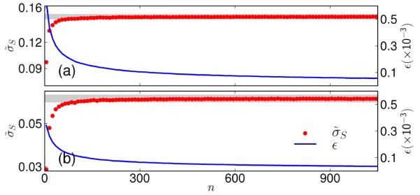
(Color online) Convergence of σ_S under sampling over windows of size n. We generate different realizations of σ_S by bootstrapping, i.e., resampling windows of size n of S_j∣j+1 values with replacement and calculating σ_S for each of the resampled window. ${\tilde{\sigma }}_S$ is the median of 10, 000 such bootstrap realizations and ϵ gives the corresponding standard error in the estimation of the median over these realizations. (a) Logistic map (b) Rössler system (in both cases, the total length of the time series is N = 4500.)

Further discussion about the analytical properties of S_j∣j+1 and its moments continues in Sec. II B. But first we present a numerical example to demonstrate that σ_S is sensitive to changes in the dimension or complexity of the attractor.

As our numerical experimentation here and in later sections will demonstrate, σ_S is extremely sensitive to changes in the dynamics, beyond the dependence on D_F elucidated above. In particular, in the presence of a dynamical transition the simple linear approximation of the local mapping may break down, so that we no longer have γ_j → 0 (or $\frac{{\beta }_j}{{\alpha }_j}\to 1$), in turn producing a large fluctuation in the values of S_j∣j+1 that is captured by σ_S. We thereby expect the statistically most significant fluctuations to indicate dynamical transitions. Indeed, as described in Sec.III, we will identify such transitions by means of statistical significance tests.

Before we discuss further analytical properties of the above introduced measure, we will first demonstrate the sensitivity of σ_S to changes in the dynamical complexity through a simple yet challenging numerical example. We will consider the coupled map

$$\begin{array}{cc}\hfill x_{i+1}& =\left(x_i+2\pi \omega \right)\text{mod}\left(2\pi \right),\hfill \\ \hfill y_{i+1}& =\frac{1}{2\pi }\left(a\cos \left(x_i\right)+b\right)\sin \left(2\pi y_i\right).\hfill \end{array}$$ (16)

This map can exhibit two distinct dynamical regimes for certain parameter regimes: one is the ordinary chaotic attractor and another is a strange non-chaotic attractor (SNA). SNA appears in various quasi-periodically driven dissipative dynamical systems [55–57] and the transition between chaos and SNA can be quite subtle. Identifying such transitions is a challenging numerical problem [58, 59]. In this example our main aim will be to show that σ_S is sensitive to changes in the dynamical complexity due to transition between these two distinct dynamical regimes. Later in Sec. III. we will further illustrate the ways in which σ_S can be employed to identify dynamical transitions.

The transitions between chaos and SNA can only be observed in the space of Lyapunov exponents of Eq. (17). The two types of Lyapunov exponents, namely, the largest transverse Lyapunov exponent Λ_T and the largest Lyapunov exponent Λ_y of the subsystem y, are given by [56, 57]

$$\begin{array}{cc}\hfill {\Lambda }_T& =\underset{n\to \infty }{\lim }\frac{1}{n}\sum _{j=1}^n\ln \mid a\cos \left(x_j\right)+b\mid ,\hfill \\ \hfill {\Lambda }_y& =\underset{n\to \infty }{\lim }\frac{1}{n}\sum _{j=1}^n\ln \mid a\cos \left(x_j\right)+b\cos \left(2\pi y_j\right)\mid .\hfill \end{array}$$ (17)

It is known that in the case of Λ_T > 0 and Λ_y < 0 we have SNA while for Λ_T > 0 and Λ_y > 0 we have a chaotic regime. In Fig. 4 (a, b) the grey band represents the transition to SNA from chaos. This transition is known to occur via on-off intermittency, whereas the grey band in Fig. 4 (c, d) highlights the transition from SNA to chaos.

FIG. 4.

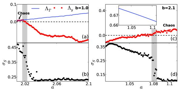
(Color online) An illustration of σ_S’s sensitivity to the changes in the dynamical complexity: identifying transition between chaos and strange non-chaotic attractor (SNA). Chaos exists when both Λ_T (largest transverse Lyapunov exponent) and Λ_y (largest Lyapunov exponent) have positive values whereas SNA exists when Λ_y is negative and Λ_T is positive. (a,c) Largest transverse Lyapunov exponent Λ_T (blue lines) and largest Lyapunov exponent Λ_y (red dots) on varying parameter a (see Eq. (17) and Eq. (18)). Transitions between chaos and SNA are highlighted by gray vertical band in all the panels. (a) Observe Λ_y becoming negative while a is increased whereas Λ_T is positive and continues to increase leading to a transition from chaos to SNA (gray band). In (b) we show σ_S (black dots) calculated from time series of x variable of Eq. (17). Observe the sharp drop in values of σ_S as the chaos converts into SNA (gray band). (c) Observe Λ_y becoming positive while a is increased whereas Λ_T is positive and continues to decrease leading to a transition from SNA to chaos (gray band). (d) The value of σ_S shows a sharp drop as SNA disappears into chaos.

We generate a short time series of length N = 4500 at 100 different values of a separated by 0.002. Then we calculate σ_S using embedding parameters m = 5 and L = 2. In Fig. 4 we have plotted σ_S with the Λ_T and Λ_y. An abrupt change in the values of σ_S would indicate a transition. Comparing Fig. 4 (a, b) we observe that as Λ_y starts to decrease and becomes negative, the values of σ_S show a simultaneous drop, signifying the dependence of σ_S on the complexity or qualitative features of the dynamics. We observe lower values of σ_S for SNA than for chaos. A similar change is observed if we reverse these transitions, i.e., going from SNA to chaos (Fig.4 (c, d)). As the values of Λ_y increase to positive values there is again a sharp drop in the values of σ_S. This example demonstrates that σ_S is able to capture even a subtle change in dynamics, like the ones that occur in transitions between SNA and chaos. In [1] we have shown that σ_S can uncover all the transitions that are induced by the variation of the parameter in a logistic map like period-chaos transitions, intermittency, chaos-chaos transitions, etc..

B. Relationship with Lyapunov spectrum

Lyapunov exponents λ_i are the most extensively used measures for a quantitative characterization of nonlinear dynamics [3–5, 23, 48]. Several dynamical invariants are conjectured in terms of them such as Lyapunov dimension. However, reliably estimating λ_i from short time series remains a challenging problem [48, 60, 61], frequently encountered in various real time systems. The main objective of this section is to understand the new measure S_j∣j+1, its mean μ_S, and variance σ_S in terms of these well known dynamical measures of Lyapunov exponents.

Suppose that Eq. (4) holds and ${\lambda }_1^j,{\lambda }_2^j,\dots ,{\lambda }_m^j$ are the eigenvalues of the Jacobian matrix Dϕ(x_j). Then the deformation of the infinitesimal ϵ_j(k) ball neighborhood of x_j in any direction i will be a multiple of exp(${\lambda }_i^j$) (see Fig. 5). Defining ${\Lambda }_i^j=\text{exp}\left({\lambda }_i^j\right)$, where ${\Lambda }_i^j$ are called the Lyapunov numbers, the local Lyapunov exponents, λ_i, are given by

$${\lambda }_i\left(n\right)=\frac{1}{n}\sum _{j=1}^n{\lambda }_i^j.$$ (18)

The global Lyapunov exponent L_i corresponding to the direction i is the asymptotic value of λ_i

$$L_i=\underset{n\to \infty }{\lim }\frac{1}{n}\sum _{j=1}^n{\lambda }_i^j.$$ (19)

If the Euclidean distance metric is used for calculation of d(x_j), a simple geometrical consideration yields

$$d\left({\mathrm{x}}_{j+1}\mid {\mathrm{x}}_j\right)={\left(\frac{1}{m}\sum _{i=1}^m{\left({\Lambda }_i^j\right)}^2\right)}^{\frac{1}{2}}d\left({\mathrm{x}}_j\right),$$

which directly leads to

$$S_{j\mid j+1}={\left(\frac{1}{m}\sum _{i=1}^m{\left({\Lambda }_i^j\right)}^2\right)}^{-\frac{1}{2}}.$$ (20)

Hence, S_j∣j+1 measures the total deformation of the ϵ_j(k) ball neighborhood of point x_j when a mapping ϕ is applied on it.

FIG. 5.

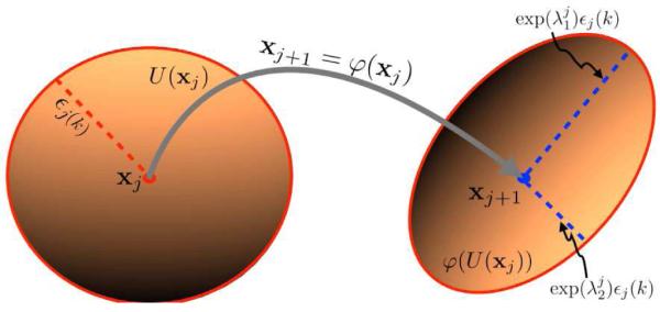
(Color online) Evolution of the ϵ(k) neighborhood of the time point x_j into an ellipsoid by the application of the smooth mapping ϕ such that x_j+1 = ϕ(x_j). The expansion or contraction in any direction i is a multiple of exp(${\lambda }_i^j$), where ${\lambda }_i^j$ are the eigenvalues of Dϕ at j.

From Eq. (20), we find that the average of S_j∣j+1 taken over a window of size n is,

$${\mu }_s=\frac{1}{n}\sum _{j=1}^n\left[{\left(\frac{1}{m}\sum _{i=1}^m{\left({\Lambda }_i^j\right)}^2\right)}^{\frac{1}{2}}\right].$$ (21)

Comparing, Eq. (21) with Eq. (18) and Eq. (19) we can conclude that μ_S will resemble the sum of the local Lyapunov exponents, approximating the sum of the global Lyapunov exponents over large n. This is shown numerically for the Logistic map in Fig. 6. In a chaotic system we always have at least one direction i such that the ${\lambda }_i^j>0$, i.e., ${\Lambda }_i^j>1$, representing the expansion in the direction i. In other directions we will either have contraction, ${\lambda }_i^j<0$, i.e., ${\Lambda }_i^j<1$ or ${\lambda }_i^j=0$, i.e., ${\Lambda }_i^j=1$. Therefore, in a chaotic system with few degrees of freedom the most dominant contribution to S_j∣j+1 in Eq. (20) comes from the largest positive eigenvalue corresponding to the expansion. Hence, for such systems μ_S will be similar to the Lyapunov exponent. In Fig. 6 we observe a strong correspondence between μ_S and the Lyapunov exponent of the logistic map. We know for certain systems the sum of the largest Lyapunov exponents is provably related to the dynamical invariants such as Lyapunov dimension, topological entropy, and information dimension (due to Kaplan-Yorke conjecture) [22, 23, 62, 63]. Therefore, we might think that μ_S could also be used in quantifying dynamics but our numerical analysis has shown that μ_S is not well suited for detecting dynamical transitions in the series because it is not sensitive in quantifying and capturing large fluctuations in S_j∣j+1. It will be better to use σ_S for this purpose, as σ_S is better suited to quantify variation in parameters of a dynamical system and corresponding changes in the dynamics, because any variation in the parameters of a dynamical system will lead to variation in the Lyapunov spectrum too. Transitions lead to large deformations of the ϵ_j(k) neighborhood, leading to large fluctuations in the magnitude of S_j∣j+1, which are then captured by σ_S. A point to note is that the global Lyapunov exponents L_i are not defined for a time series with a transition, due to the constraints imposed by ergodicity.

FIG. 6.

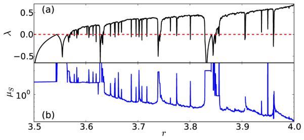
(Color online) Correspondence between μ_S (blue line in (b)) and the Lyapunov exponent λ (black line in (a)) for the logistic map. The parameters used for this figure are the same as used for Fig. 2.

In order to get further insights into the properties of σ_S we take a look at the distribution of S (dropping subscript for simplicity) over window size n of vectors, P (S, n). Since the ${\lambda }_i^j$ are in a sense random numbers for chaotic systems, and the expression of S, Eq. (20) consists of a summation over ${\Lambda }_i^j=\text{exp}\left({\lambda }_i^j\right)$, therefore, the central limit theorem implies that S follows a Gaussian distribution at least asymptotically. Following [22], we find that asymptotically P (S, n) has the following general analytical form,

$$P\left(S,n\right)~\frac{1}{\sqrt{2\pi n{\Phi }^n\left(S\right)}}\text{exp}\left(-n\Phi \left(S\right)\right),$$ (22)

where Φ(S) is a convex quadratic function with minimum zero, occurring at S = μ_S, i.e., Φ(μ_S) = 0, Φ′(μ_S) = 0, Φ^″(μ_S) > 0. Expanding Φ(S) around μ_S and neglecting higher order terms, we write Eq. (22) as,

$$P\left(S,n\right)~\frac{1}{\sqrt{2\pi n{\Phi }^{″}\left(S\right)}}\text{exp}\left(-n{\Phi }^{″}\left(S\right)\frac{{(S-{\mu }_S)}^2}{2}\right),$$ (23)

which gives a familiar looking form of a Gaussian distribution. Then

$${\sigma }_S={\left(n{\Phi }^{″}\left(S\right)\right)}^{-1∕2}.$$ (24)

A similar expression for distribution and variance could also be written for the local Lyapunov exponents [22], where Φ(λ_i) is known as the spectrum of the local Lyapunov exponents and can be used for characterising the dynamics of the system [64–66]. So as an analogy we propose that Φ(S) can also be used to characterise the dynamics. The distribution of S for different types of dynamics may follow a Gaussian distribution of the type P (S, n) asymptotically but each type of dynamics must correspond to unique μ_S and σ_S. This is because of the fact that each type of dynamics has a unique ϕ (see Eq. (4)) and hence unique eigenvalues and the corresponding deformations and values of S should also be unique. In future research we intend to develop a method based on estimation of Φ(S) to classify distinct dynamics.

III. DYNAMICAL TRANSITION INDUCED BY CO-EVOLVING PARAMETERS

In the numerical example above, values of σ_S could distinguish two distinct chaotic regimes and SNA, demonstrating that σ_S can be used to distinguish different types of dynamics. A similar example about the capability of σ_S in identifying distinct dynamics was presented in [1] for the logistic map, where σ_S was used to uncover all of the transitions induced there by variation of the parameter in the map, including period-chaos transitions, intermittency, and chaos-chaos transitions. An important point is that in these examples we had access to a whole time series at each value of the parameter. However, in many applications we do not have the luxury of a whole time series being available at a single value of the control parameters; rather, the more common real-world situation involves control parameters co-evolving with the system dynamics [13, 24–26]. In such cases, we only have very few points available at a particular value of the control parameter. For example, in the study of palaeoclimate, we have few observations of a climate variable via proxies, while the parameters driving climate like solar insolation co-evolve with these climate variables in time leading to transitions in the dynamics [1, 11, 17, 26, 30]. Other examples of such situations are readily imagined in social dynamics, where we have very few observation of social indices while the parameters driving social dynamics, like economic and political factors, coevolve with variables of interest [13, 18–20]. A further example is in neuroscience, where event-related potentials (ERP) measured by electroencephalography (EEG) show several distinct dynamical behaviors as a response to changing stimuli [67, 68].

As a conceptual model for studying such transitions in the presence of co-evolving parameters, we consider

$$\stackrel{.}{\mathrm{y}}=f\left(\mathrm{y},\zeta \left(t\right)\right),$$ (25)

where y is a set of variables of a dynamical system and ζ(t) is a parameter evolving in time. A variety of qualitative changes in the dynamics of the system may be generated by the passing of ζ(t) through a bifurcation point or even the rate of change of ζ(t). Some of the system changes may be subtle, such as shifting from one regime of complex chaotic dynamics to another chaotic dynamics of higher or lower complexity [3, 17, 24–26]. In the numerical examples following this section, we let the parameter simultaneously evolve with variables of the system, in order to better test the method for practical utility in real systems.

A statistical test for assisting with a more automatized identification of dynamical transitions presented in [1] is briefly described here again for convenience. To test the relative statistical significance of two values of σ_S belonging to distinct dynamics we use a bootstrapping procedure where we randomly draw n values with replacement from the series of S_j∣j+1, where n is the window size used in calculation of σ_S. Repeating this procedure several thousand times, we generate an ensemble of values of σ_S and interpret the 0.05 and 0.95 quantiles of this ensemble as the 90% confidence bounds. The values of σ_S outside this bound are then classified as belonging to dynamics of two distinct complexity with 90% confidence. The time band over which the crossover between the two levels occurs contains the point of dynamical transition. The points with lower values of σ_S may be regarded as belonging to dynamical regimes which are relatively more stable and lower in dynamical complexity.

A. Identifying drift in the dynamics (nonstationarity)

In order to explore the challenge of identifying a continuous drift in the dynamics of a time series, we consider the generalized Baker’s map [69], with a time series generated following the procedure described in [6]:

$$\begin{array}{cc}\hfill \text{if}{v}_i\le \alpha :u_{i+1}& =\beta u_i,v_{i+1}=v_i∕\alpha ,\hfill \\ \hfill \text{if}{v}_i>\alpha :u_{i+1}& =0.5+\beta u_i,v_{i+1}=\frac{\left(v_i-\alpha \right)}{\left(1-\alpha \right)},\hfill \end{array}$$ (26)

with Lyapunov exponents

$${\lambda }_1=\alpha \ln \frac{1}{\alpha }+\left(1-\alpha \right)\ln \frac{1}{1-\alpha },$$ (27)

$${\lambda }_2=\ln \beta .$$ (28)

Introducing a drift in the parameter β as done in [6], we generate a time series of length 15, 000 with fixed α = 0.4 and varying β = i/15, 000. We remove the trend from the resulting time series by the transformation

$$x_i=\frac{w_i-{\langle w\rangle }_k}{\sqrt{{\langle {(w_i-{\langle w\rangle }_k)}^2\rangle }_k}},$$

where w_i = u_i + v_i and averages are taken locally over the k = 50 nearest times.

Ignoring the initial transient, we consider only a relatively short section of the time series, 1000 ≤ i ≤ 7000 (cf. the 40, 000 data points used in [6]). The top panel in Fig. 7 shows the times series and the middle panel shows the evolution of λ₂. Observe that there is no visibly apparent trend in the time series even though λ₂ is continuously evolving. Using embedding parameters m = 5 and L = 2, we observe in Fig. 7 that values of σ_S drift from significantly higher values (orange dots) to significantly lower ones (green dots), indicating a dynamical drift that has occurred during this time interval. This evolution of σ_S can be described by a quadratic fit, as shown in Fig. 7 (lowest panel) with thick red line. Given the limited range of β here, λ₂ = ln β can be approximated by quadratic polynomial in β. Therefore, the dynamical drift defined by λ₂ should be visible in the form of a quadratic trend in any other measure of dynamical complexity. It seems σ_S is very well able to capture this feature of the dynamics.

FIG. 7.

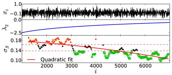
(Color online) Identifying drift in the dynamics of the Baker’s map with continuously changing parameter β. As indicated in Eq. (27), λ₁ is constant with respect to β. In contrast, λ₂ = ln β. We observe σ_S changing from significantly higher values to significantly lower values as the time progresses. A quadratic fit describes this evolution (red curve), indicating the nonlinear change of parameter of the system.

B. Transition between transient chaos and Lorenz’s attractor

In order to explore a continuous-time example with a transition from transient chaos to a chaotic attractor, we next consider the Lorenz system

$$\begin{array}{cc}\hfill \stackrel{.}{x}& =a\left(y-z\right),\hfill \\ \hfill \stackrel{.}{y}& =x\left(\gamma -z\right)-y,\hfill \\ \hfill \stackrel{.}{z}& =\mathit{xy}-\mathit{bz},\hfill \end{array}$$ (29)

with a = 10 and b = 8/3. The chaotic Lorenz attractor exists for γ > 24.74, whereas transient chaos exists for 13.9 < γ < 24.06. For the transition zone 24.06 < γ < 24.74, there is a coexistence of three attractors: two steady states and one a chaotic attractor [70]. The transient chaos disappears due to a crisis at γ ≈ 24.06 and Lorenz’s attractor emerges as the only possible stable attractor due to a subcritical Hopf bifurcation at γ ≈ 24.74. We investigate a time series of the x variable as generated by a fourth-order Runge-Kutta numerical solution with time step h = 10⁻³ that is sampled every 10³ time steps. We sample 6, 000 such time points during which γ is varied linearly from 23.5 to 25.25 (γ = γ₀ + 2.92 × 10⁻⁴t, where γ₀ = 23.5 and t is the integration time). This variation leads the system to pass from transient chaos to a transition zone (crisis and subcritical Hopf transitions) to the formation of of the Lorenz attractor (Fig. 8).

FIG. 8.

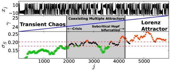
(Color online) Formation of Lorenz’s attractor, when parameter γ is varied from 23.5 to 25.25 (see Eq. (29)). When γ < 24.06, transient chaos exist whereas 24.06 < γ < 24.74 is a transition zone where multiple attractors coexist and for γ > 24.746 only Lorenz’s attractor exists. The σ_S distinguishes between these three regions, for γ < 24.06 green open squares indicates low complexity dynamics, for γ > 24.74 only orange dots exist indicating higher complexity dynamics. In between these two regions we have a state where multiple attractors coexist, indicated by jumps in the values of σ_S below and above the significance bands (red dotted horizontal lines). The thick black vertical lines are drawn at the times points when γ ≈ 24.06 (crisis) and γ ≈ 24.74 (subcritical Hopf bifurcation)

To calculate σ_S for this example we have used m = 10, L = 10 and a window size of 300 with 90% overlap. A detailed explanation for our choice of rather higher values of embedding parameters is provided in Sec. III F. The calculated values of σ_S are shown in the lowest panel of Fig. 8. We observe lower values of σ_S (green open squares) predominantly below the confidence bound for transient chaos and higher values (orange dots) predominantly above the confidence bound for the Lorenz attractor, distinguishing the two dynamical regimes in this time series. The transition zone (grey shaded region) not only contains multiple transitions but also multiple attractors, which is also reflected in the values of σ_S jumping between green open squares and orange dots. Due to the fact that the formation of an attractor is temporally delayed [71], and we also lose a few initial points due to windowing and embedding, the transitions are typically rightward shifted, as expected.

C. Abrupt transitions between chaos and intermittent chaos

We next explore abrupt jumps between distinct dynamical regimes, by way of an Ikeda map. In this map, two different kinds of chaos can be observed by changing one of the parameters. The first type of chaos is distinguished from the second one by the existence of intermittent bursts of activity. The phenomenon that describes this feature is called an interior crisis or an attractor merging crisis, where a chaotic attractor suddenly widens while still spending long stretches of time within the region of the former attractor [72–74]. The Ikeda map is given by

$$z_{j+1}=a+{\mathit{bz}}_j\text{exp}\left(i\kappa -\frac{i\eta }{1+{\mid z_j\mid }^2}\right)$$ (30)

with z = x+iy complex [22, 75]. We consider the parameters a = 0.85, b = 0.9, and κ = 0.4, for which we will have chaos for η < η_c ≐ 7.2688489 and intermittent chaos above the critical value (η > η_c) [76]. We here make η abruptly change between η = 7.2 (precrisis) and η = 7.4 (postcrisis) in every 100th iteration of the map to generate a time series of the variable y_j = Im(z_j) of length N = 500 (i.e., containing four transitions between precrisis chaos and postcrisis intermittent chaos in a relatively short time series).

In Fig. 9 we observe that σ_S (calculated with window size n = 50 and embedding parameters m = 5 and L = 5) correctly identifies these four transitions in the time series of the variable y_j. We note that σ_S has higher values (orange dots) for intermittent chaos (η = 7.4) and lower values (green open squares) for chaos (η = 7.2). The width of the grey bands is equal to n and they are centered at the transitions and hence the jump in the values of σ_S between different dynamical regimes is expected to occur within these bands. This example also illustrates the capability of the method to identify transitions even in the presence of short lived nonstationarity in the form of intermittent burst in the dynamics.

FIG. 9.

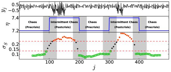
(Color online) Identifying abrupt transition between chaos and intermittent chaos induced by an interior crisis. The iterations of the Ikeda map (Eq. 30) for η = 7.2 and η = 7.4 belong to the precrisis chaos and the postcrisis intermittent chaos respectively. y_j is the imaginary part of z_j. Observe the values of σ_S jumping between the green color markers (open squares) and the orange color markers (dots) as η is abruptly changed between two dynamical regimes. The vertical grey bars indicate the region where transitions should be found and their width is equal to the window size n.

D. Tolerance of the measure against observational noise

To test the influence of observational noise on FLUS, we again consider the example of the Rössler model, Eq. (9). In this system, two topologically distinct attractors exist, namely spiral type chaos for a = 0.32 and screw type chaos for a = 0.38. Somewhere in the interval 0.32 < a < 0.38, a transition from screw to spiral type chaos occurs via the formation of a homoclinic orbit [77, 78].

We generate a test time series for our method by varying the control parameter a by $a\left(t\right)=0.32+0.07\mid \sin \left(\frac{\pi }{600}t\right)\mid$ where t is the integration time, and we have used a fourth-order Runge-Kutta integrator with h = 10⁻³. We sample 6, 000 points of the x-component separated in time by 200h. The control parameter a crosses the transition point four times during this time series [see Fig. 10(c)]. While this example system was also discussed in [1], we do so here in the context of observational noise (the present subsection) and missing values (in the next subsection).

FIG. 10.

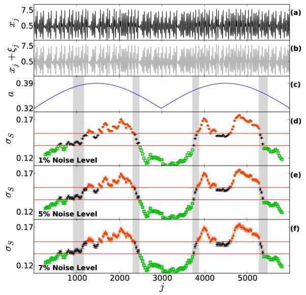
(Color online) Test the effect of presence of observational noise on the method: (a) x_j are values of x variable of Eq. 9 sampled at time step j, (b) shows the effect of adding white noise to x_j. (c) shows the variation of control parameter a, note the crossing of four grey bands by the parameter a. These grey band represent the four dynamical transition that take place when a crosses the value close to 0.38. The width and location of these bands is the same as in the noiseless case presented in [1]. (d-f) shows the variation of σ_S with three different levels of noise added to the signal. For 1% we see the smallest error bars and all the four transitions are clearly visible, i.e., crossing of significane band by values of σ_S right between the grey bands. In higher noise levels the transitions are still intact but with increasing error bars.

We add simple white noise to this time series, adding to each time point a random variable ξ from a normal distribution with mean 0 and standard deviation σ(ξ) = ησ(x), where σ(x) is the observed standard deviation of the original time series [see Fig. 10(b)]. We vary the strength of noise by varying η: for instance, η = 0.01 corresponds to a 1% noise level in the signal. We test the tolerance of the measure against three different noise levels here, viz. 1%, 5%, and 7% [see Fig. 10(d-f)]. The error bars on the values of σ_S are obtained by generating 1, 000 different realizations of noise at each level. We have replaced the significance levels from dotted red lines to solid red lines, as these are the mean of the significance levels for the different realizations of the noise. In Fig. 10(d-f) we observe that all the transitions seem to remain intact for all the different levels of noise. This is a clear indication that this method is robust against nominal levels of noise. We have also attempted the above numerical experiment with some other models, and the results of those experiments also demonstrate similar robustness of this method against nominal levels of noise. The embedding parameters used for every level of noise are exactly the same: m = 10 and L = 15 with window size of 300 and 90% overlap. These parameters are also the same as used in [1] to discuss the same example system in the absence of noise.

E. Strategy for treatment of missing values

Apart from shortness of the data, another central problem which surrounds data analysis is irregular sampling or missing values [79–81]. This is a common problem in fields such as astronomy, medical, earth, and social sciences [79–84]. We here propose a strategy to deal with missing values while using FLUS. To generate a test time series, we consider the same Rössler model as used in the previous section and randomly remove some of the values in the time series. The number of time points removed from the time series are given in terms of percentage of missing values. A straightforward application of the FLUS method will not work in such a case, due to the incompatibility of embedding a time series in delayed coordinates with missing values. The first step of our strategy for dealing with treatment of missing values involves replacing the missing values with a flag (e.g. a NaN character). Then we continue to embed the time series in time delayed coordinates, with some of the coordinates just being the flags. But this would make the numerical calculation of a distance metric impossible. To get over this issue we recommend to use of the Chebyshev distance, rather then Euclidean distance as done elsewhere in this work. Chebyshev distance between two vectors x_j and x_l is given by $\Vert {\mathrm{x}}_j-{\mathrm{x}}_l\Vert =\underset{i}{\max }\left\{\mid x_j^i-x_l^i\mid \right\}$, where $x_j^i$ is the ith component of the vector x_j. It ignores the non-numerical flags and maximum is only calculated over the numerical values. Thus, it returns non-numerical values only in the rare case when all the components of both the vectors are non-numerical flags. Using the same delay and embedding dimensions as in the previous section, we present the result at different amounts of missing values in Fig. 11 (c-e). The error bar on the values of σ_S were obtained from 1000 different realizations of missing values. The solid horizontal red lines are again the mean significance levels for different realizations of missing values. In Fig. 11 we observe that the above strategy seems to work with a reasonable amount of missing values in the data. The embedding parameter used in this case were exactly the same as used in previous example.

FIG. 11.

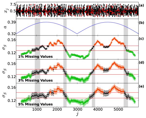
(Color online) Testing the effect of missing values on the method: (a) Red points represent the time points missing from the dynamics (black points) of the Rössler system at the level of 5% missing values. The transitions highlighted by grey bands are introduced by changing the parameter a in Eq. 9 as described above in Sec. III D. (c-e), showing the variation of σ_S at different levels of missing values, in all the three we observe the transitions to remain intact. An important point to note is that even on using Chebyshev distance, there is no structural change in evolution of σ_S compared to the previous example (See Fig. 10).

F. A note about embedding parameters, window size and length of the time series

In the examples above, we have used a rather high embedding dimension, which is due to the fact that the systems we are considering have one of its parameters varying with time (such as Bakers’ map, and Lorenz system with a drift, and Rössler system with nonlinear transitions). This converts the systems into non-autonomous systems. Taken’s theorem is not valid for such a system. Hence, we cannot take the embedding dimension 2m + 1 as prescribed by the Taken’s theorem (m is the known dimension of the system) [43, 85]. Though there is no specific embedding theorem for such systems, heuristic arguments in [86] state that a proper choice for the embedding dimension should be larger than 2(m + P) where P is the number of time varying parameters of the system. It has been suggested that this technique of “overembedding” a time series helps in overcoming both nonstationarity and noise effects [86, 87]. We will continue using high embedding dimension in the next section, where we apply our method to the analysis of crime record’s time series, as these time series have originated from a system (society) which is not only high dimensional but also a large parameter space. So, 2(m + P) must be a large number. In the crime record’s time series used below, apart from visible non-stationarity the time series also have a high amount of noise which is also visible by eye and via its power spectrum. Hence, a high embedding dimension is an appropriate choice.

In Fig. 3 we have shown a quick convergence of σ_S on taking large enough window sizes, which in turn gives the measure dependence on the structure of the attractor through the effective dimension D_F. By taking overlapping windows, we avoid reducing the amount of data appreciably. The presented method differs in one very basic aspect from other methods, in particular those based on recurrence properties. In many of them one first takes a window over the data (or embedded vectors) and then calculate some measure based on the recurrence property [2, 7, 9, 10, 88]. This creates a relationship between windowing, dimension and delay. In our method we follow a different approach, first the recurrence distances of a point over the whole time series are calculated and, then, by comparing each consecutive time point, we calculate the measure S_j∣j+1 for each point. Up to this step we have no windowing. In the next step we calculate the fluctuations in this measure by taking windows. The way we have defined the significance test, the window size now helps in resolving time scales on which we wish to see the transitions. The real task of windowing is to give control over resolving time scales for transitions.

Another crucial point is the minimum length of the time series required to apply this method. The only requirement for the method to work is that we should have enough points so that a convergent value of σ_S can be obtained. We observe the quick convergence of σ_S in Fig. 3(a-b), where σ_S converges over only a few hundred points. In general, a minimum of few hundred points should be sufficient to apply this method. An exception to this requirement may occur in a case where the rate of occurrence of transitions is faster than the time the attractor takes to set in.

IV. APPLICATION TO SOCIAL DYNAMICS

Now we present an application of our method to an observed time series in social dynamics. Crime rates in society might be interpreted as following some nonlinear dynamics and affected by political, economic, and social situations [89]. Analytic methods of time series analysis and agent based modeling have been used to predict and quantify the evolution of crime rates in different settings and societies [90–94]. Various methods from the rich paradigm of nonlinear time series analysis do not appear to have been applied to available data sets of crime records. We here analyze time series of robberies and homicides in the United States from 1975 to 1993 with monthly resolution. With this analysis we attempt to understand the nature of relationship if any between unemployment and robberies, and unemployment and homicides over this period [91, 95, 96].

A. Data source

The source of data studied here on monthly robberies and monthly homicides is ICPSR (Inter-university Consortium for Political and Social Research) study 6792 (Uniform Crime Reports: Monthly Weapon-Specific Crime and Arrest Time Series, 1975-1993). The source of unemployment data is the US Bureau of Labour Statistics (http://www.bls.gov/data/), using the monthly levels of unemployment for the whole US for the period 1975-1993. In Fig. 12 (a) and Fig. 13 (a), black lines correspond to monthly robberies and monthly homicides respectively and blue dotted lines represent the unemployment rate over the same period. For the results below, we have removed the linear trend from monthly robberies and monthly homicides time series by subtracting a linear least squares fit to the data.

FIG. 12.

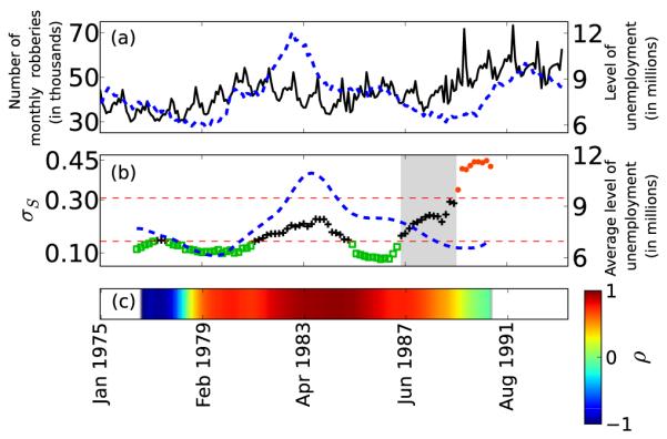
(Color online) (a) Black line indicates the monthly robberies in the US between 1975 to 1993, whereas the blue dotted line is the monthly unemployment rate between the same period. (b) Values of σ_S calculated for monthly robberies time series, represented by green open squares, black + signs and orange dots. The blue dotted line is the average values of monthly unemployment rate, calculated exactly with the same window sizes as used for σ_S. Note the change in the values of σ_S from green open squares to orange dots, representing a transition from one dynamical regime to other, as also highlighted with the grey band. (c) Continuous color variation shows running windowed linear cross-correlation ρ between average values of monthly unemployment rate and values σ_S. Observe the high correlation between the two until 1987.

FIG. 13.

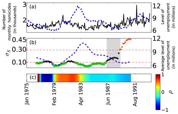
(Color online) (a) Black line indicates the monthly homicides in the US between 1975 to 1993, whereas the blue dotted line is the monthly unemployment rate between the same period. (b) Values of σ_S calculated for monthly homicides time series, represented by green open squares, black + signs and orange dots. The blue dotted line is the average values of monthly unemployment rate, calculated exactly with the same window sizes as used for σ_S. Note the change in the values of σ_S from green open squares to orange dots, representing a transition from one dynamical regime to other, as also highlighted with the grey band. (c) Continuous color variation shows running windowed linear cross-correlation ρ between average values of monthly unemployment rate and values σ_S. Observe the low correlation between the two for almost over the whole of time period.

B. Results

The calculation of σ_S for the monthly robberies and homicides time series was done using a window size of 20 months with 90% overlap, embedding dimension 12, and delay of 3, plotted in Fig. 12(b) and Fig. 13(b). As emphasised in the discussion above, higher values of σ_S correspond to greater variability or complexity in the dynamics; while low values correspond to low complexity in the dynamics. For the monthly robberies time series in Fig. 12(b) we observe low values of σ_S until 1982 (green open squares). Between 1983-1985 we also observe lower values of σ_S but in a statistically insignificant regime (black plus signs). Then close to 1987 there is a significant increase in the values of σ_S (orange dots) and the values cross the significance band during a transition between the period 1987–1990 (highlighted by a grey band). We uncover a similar transition in Fig. 13(b) occurring close to 1987 (see the grey band in both figures covering the period 1987–1990.)

If we closely observe the original time series of robberies and homicides, then it is visible even to the naked eye that there are higher variabilities and larger fluctuations after this period. A fact to be noted here is that crimes in the US across all categories of crime started to drop in the 1990’s and this drop has continued since [97–100]. Several reasons have been hypothesized for this decrease, including increased incarceration [101], more police [102], the decline of crack use [103], legalized abortion [97], improvement in the quantity and quality of security [99] and changing demographics [100]. Our time series analysis above only brings forward the point that some fundamental change in the dynamics of crime in the US occurred in the late 1980’s and early 1990’s, leading to continuous drop in the crime rate in the following decades.

In Fig. 12 (c) and Fig. 13 (c), the continuous color variation gives the cross correlation ρ between σ_S and unemployment rate averaged over exactly the same time windows as σ_S. The blue curves in the middle panels of Fig. 12 and Fig. 13 correspond to this averaged unemployment rate. In the case of unemployment and robberies, we observe high positive values of cross correlation (ρ ~ 1.0) between the two curves from 1979 to 1989 and then an abrupt breakdown of this correlation, indicating some fundamental shift in the crimes related to robberies around this time. In our second case of homicides, however, we do not observe any such relation between unemployment and homicides: the values of cross correlation between σ_S and average unemployment are rather low starting in the mid 1980s, fluctuating between negative and positive values. That is, the signals of unemployment rate driving variability and complexity in dynamics of robberies before the 1990’s are quite apparent but they do not seem to play a similarly significant role in homicides.

Sociologists have pointed out that the relationship between unemployment and robberies is a rather complex one: increasing unemployment increases the criminal motivation (unemployed individuals are more motivated to indulge in robbery for their financial needs and survival) but it also decreases the criminal opportunity (more men start to stay at home, so less opportunity for criminals to break into homes), creating a counter balancing effect [104]. Hence, we cannot expect a linear relationship between both. We have also not observed a strong linear correlation (see Fig. 14) or a Granger causal relationship between these two variables. What our above analysis shows is that unemployment may have been driving the complexity or variability in the dynamics of robberies prior to the late 1980’s and early 1990’s. The breakdown in this relationship corresponds to a time period when the crime rate in the US started to steadily drop, due to several reasons discussed in detail in the references [97–103].

FIG. 14.

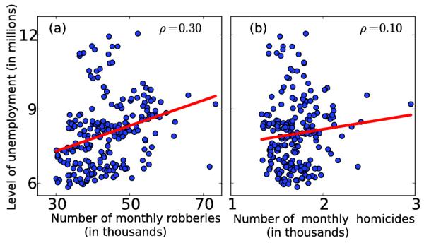
(Color online) (a) Scatter plot between the level of unemployment and monthly robberies. (b) Scatter plot between the level of unemployment and monthly homicides. ρ is the cross-correlation between the plotted variables and the red color line is the linear fit. Note the low correlations between the plotted variables in both (a) and (b).

An important perspective in criminology has been conflict theory, where it is considered that economic deprivations influence crime rates [92], but there does not exist a conclusive empirical support for this relationship [95, 96, 105]. In our analysis, if we treat the unemployment rate as being one of the economic indicators then we observe an episodic relationship between robberies and unemployment but the same cannot be said for homicides. Undoubtedly multiple interconnected factors including economic indicators drive crime rates. It is not possible to discern all such relationships with our method. To accept or reject the economic deprivations perspective of crime, one would need to do an extensive analysis of different social and economic indicators. Our method can only help in identifying certain fundamental shifts or transitions in the dynamics of the system at different temporal scales, though some of those transitions would be in the realm of speculation until and unless we have some independent means to verify them.

V. CONCLUSION

Developing a set of methods that can be used to distinguish distinct dynamical regimes and transitions between them in a given time series has been a challenge in nonlinear time series analysis with wide applicability in a variety of fields. We have recently proposed the new method FLUS, based on computation of nonlinear similarities between time points of a univariate time series [1]. FLUS is robust, automatized, and computationally simple and can be used even in cases with shorter time series, or missing values, or observational noise. Here we have presented some new analytical findings, where we have related this measure to some classical concepts in nonlinear dynamics such as attractor dimensions and Lyapunov exponents. We have shown that the new measure has linear dependence on the variation of change in dimensionality or complexity of the attractor. Also, it measures the variance of the sum of the Lyapunov spectrum. One of the problems we have studied in detail with this method is identification of transitions in dynamics when the parameters of the system are also evolving with dynamics. The proposed method is able to identify these most subtle of transitions, even including those where the evolution of parameters induces only a drift or nonstationarity in the dynamics. Also, employing a wide variety of prototypical model systems we have demonstrated the practical usefulness of this method.

Furthermore, we have used this method to analyze a time series from social dynamics, studying time series of US crime from 1975 to 1993. In doing so we have attempted to understand the nature of the relationship between crime rates (robbery and homicides) and unemployment levels during this period. We have found a dynamical transition in the late 1980’s in both homicide and robbery rates and also found the dynamical complexity in robbery rates was driven by unemployment before this transition in 1990’s. As demonstrated above, FLUS could be useful in such analysis and in other endeavours where similar questions could arise.

References

- [1].Malik N, Zou Y, Marwan N, Kurths J. Europhysics Letters. 2012;97:40009. [Google Scholar]
- [2].Marwan N, Romano M, Thiel M, Kurths J. Phys. Rep. 2007;438:237. [Google Scholar]
- [3].Kantz H, Schreiber T. Nonlinear Time Series Analysis. 2nd ed Cambridge University Press; Cambridge: 2004. [Google Scholar]
- [4].Small M. Applied Nonlinear Time Series Analyses. World Scientific; 2005. [Google Scholar]
- [5].Abarbanel H. Analysis of Observed Chaotic Data. 1st ed Springer; 1996. [Google Scholar]
- [6].Schreiber T. Phys. Rev. Lett. 1997;78:843. [Google Scholar]
- [7].Donges JF, Donner RV, Rehfeld K, Marwan N, Trauth MH, Kurths J. Nonlinear Processes in Geophysics. 2011;18:545. [Google Scholar]
- [8].Livina VN, Lenton T. Geophys. Res. Lett. 2007;34:L03712. [Google Scholar]
- [9].Donges JF, Donner RV, Trauth MH, Marwan N, Schellnhuber HJ, Kurths J. PNAS. 2011;108:20422. doi: 10.1073/pnas.1117052108. [DOI] [PMC free article] [PubMed] [Google Scholar]
- [10].Marwan N, Donges JF, Zou Y, Donner RV, Kurths J. Phys. Lett. A. 2009;373:4246. [Google Scholar]
- [11].Lenton TM, Held H, Kriegler E, Hall JW, Lucht W, Rahmstorf S, Schellnhuber HJ. PNAS. 2008;105:1786. doi: 10.1073/pnas.0705414105. [DOI] [PMC free article] [PubMed] [Google Scholar]
- [12].Schütz N, Holschneider M. Phys. Rev. E. 2011;84:021120. doi: 10.1103/PhysRevE.84.021120. [DOI] [PubMed] [Google Scholar]
- [13].Scheffer M. Critical Transitions in Nature and Society. Princeton University Press; 2009. [Google Scholar]
- [14].Lehnertz K, Elger CE. Phys. Rev. Lett. 1998;80:5019. [Google Scholar]
- [15].Venegas J, Winkler T, Musch G, Melo MV, Layfield D, Tgavalekos N, Fischman A, Callahan R, Bellani G, Harris R. Nature. 2005;434:777. doi: 10.1038/nature03490. [DOI] [PubMed] [Google Scholar]
- [16].McSharry PE, Smith LA, Tarassenko L. Nature Med. 2003;9:241. doi: 10.1038/nm0303-241. [DOI] [PubMed] [Google Scholar]
- [17].Ashwin P, Wieczorek S, Vitolo R, Cox P. Phil. Trans. R. Soc. A. 2012;370:1166. doi: 10.1098/rsta.2011.0306. [DOI] [PubMed] [Google Scholar]
- [18].May R, Levin S, Sugihara G. Nature. 2008;451 doi: 10.1038/451893a. [DOI] [PubMed] [Google Scholar]
- [19].Mantegna RN, Stanley HE. An Introduction to Econo-physics: Correlations and Complexity in Finance. Cambridge University Press; Cambridge, UK: 1999. [Google Scholar]
- [20].Chakrabarti BK, Chakraborti A, Chatterjee A. Econophysics and Sociophysics : Trends and Perspectives. Wiley-VCH; Berlin: 2006. [Google Scholar]
- [21].Chakrabarti BK, Acharyya M. Rev. Mod. Phys. 1999;71:847. [Google Scholar]
- [22].Ott E. Chaos in Dynamical Systems. 2nd ed Cambridge University Press; Cambridge: 2002. [Google Scholar]
- [23].Ruelle D. Chaotic evolution and strange attractors - The statistical analysis of time series for deterministic nonlinear systems. Cambridge; Cambridge, UK: 1989. [Google Scholar]
- [24].Guckenheimer J, Holmes P. Nonlinear Oscillations, Dynamical Systems, and Bifurcations of Vector Fields. Springer; 1983. [Google Scholar]
- [25].Benoît E, editor. Dynamic bifurcations. Lecture Notes in Mathematics. Vol. 1493. Springer-Verlag; Berlin, Germany: 1991. [Google Scholar]
- [26].Kuehn C. Physica D. 2011;240:1020. [Google Scholar]
- [27].Ditlevsen PD, Kristensen MS, Andersen KK. Journal of Climate. 2005;18:2594. [Google Scholar]
- [28].Ditlevsen PD, Johnsen S. Geophys. Res. Lett. 2010;37:L19703. [Google Scholar]
- [29].Ganopolski A, Rahmstorf S. Phys. Rev. Lett. 2002;88 doi: 10.1103/PhysRevLett.88.038501. [DOI] [PubMed] [Google Scholar]
- [30].Levermann A, Schewe J, Petoukhov V, Held H. PNAS. 2009;106:20572. doi: 10.1073/pnas.0901414106. [DOI] [PMC free article] [PubMed] [Google Scholar]
- [31].Marwan N, Schinkel S, Kurths J. EPL (Europhysics Letters) 2013;101:20007. [Google Scholar]
- [32].Steyn-Ross DA, Steyn-Ross M, editors. Modeling Phase Transitions in the Brain. Springer; 2010. [Google Scholar]
- [33].Tredicce JR, Lippi GL, Mandel P, Charasse B, Chevalier A, Picque B. Am. J. Phys. 2004;72 [Google Scholar]
- [34].Held H, Kleinen T. Geophys. Res. Lett. 2004;31:L23207. [Google Scholar]
- [35].Guttal V, Jayaprakash C. Theoret. Ecol. 2008;2:3. [Google Scholar]
- [36].Iwayama K, Hirata Y, Suzuki H, Aihara K. Nonlinear Theory and Its Applications, IEICE. 2013;4:160. [Google Scholar]
- [37].Gao Z, Jin N. Chaos. 2009;19:033137. doi: 10.1063/1.3227736. [DOI] [PubMed] [Google Scholar]
- [38].Gao Z-K, Jin N-D, Wang W-X, Lai Y-C. Phys. Rev. E. 2010;82:016210. doi: 10.1103/PhysRevE.82.016210. [DOI] [PubMed] [Google Scholar]
- [39].Zou Y, Heitzig J, Donner R, Donges J, Farmer J, Meucci R, Euzzor S, Marwan N, Kurths J. Europhysics Letters. 2012;98:48001. [Google Scholar]
- [40].Donner RV, Small M, Donges JF, Marwan N, Zou Y, Xiang R, Kurths J. Int. J. Bifurc. Chaos. 2011;21:1019. [Google Scholar]
- [41].Donner RV, Heitzig J, Donges JF, Zou Y, Marwan N, Kurths J. Eur. Phys. J. B. 2011;84:653. [Google Scholar]
- [42].Gibson JF, Farmer JD, Casdagli M, Eubank S. Physica D. 1992;57:130. [Google Scholar]
- [43].Packard NH, Crutchfield JP, Farmer JD, Shaw RS. Phys. Rev. Lett. 1980;45:712. [Google Scholar]
- [44].Zou Y, Pazó D, Romano MC, Thiel M, Kurths J. Phy. Rev. E. 2007;76:016210. doi: 10.1103/PhysRevE.76.016210. [DOI] [PubMed] [Google Scholar]
- [45].Arnhold J, Grassberger P, Lehnertz K, Elger C. Physica D. 1999;134:419. [Google Scholar]
- [46].Termonia Y, Alexandrowicz Z. Phys. Rev. Lett. 1983;51:1265. [Google Scholar]
- [47].Pettis KW, Bailey TA, Jain AK, Dubes RC. IEEE Transactions on Pattern Analysis and Machine intelligence PAM-1(1) 1979:25. doi: 10.1109/tpami.1979.4766873. [DOI] [PubMed] [Google Scholar]
- [48].Parker TS, Chua L. Practical Numerical Algorithms for Chaotic Systems. Springer-Verlag; 1989. [Google Scholar]
- [49].Badii R, Politi A. J.Stats. Phys. 1985:40. [Google Scholar]
- [50].Grassberger P. 1985;107A [Google Scholar]
- [51].Grassberger P, Procaccia I. Physica D Nonlinear Phenomena. 1983;9:189. [Google Scholar]
- [52].Grassberger P, Procaccia I. Phys. Rev. Lett. 1983;50:346. [Google Scholar]
- [53].Grassberger P. Phys. Lett. A. 1983;97:227. [Google Scholar]
- [54].Gao JB. Phys. Rev. Lett. 1999;83:3178. [Google Scholar]
- [55].Grebogi C, Ott E, Pelikan S, Yorke JA. Physica D: Nonlinear Phenomena. 1984;13:261. [Google Scholar]
- [56].Yalçinkaya T, Lai Y-C. Phys. Rev. E. 1997;56:1623. [Google Scholar]
- [57].Lai Y-C. Phys. Rev. E. 1996;53:57. [Google Scholar]
- [58].Ngamga EJ, Senthilkumar DV, Prasad A, Parmananda P, Marwan N, Kurths J. Phys. Rev. E. 2012;85:026217. doi: 10.1103/PhysRevE.85.026217. [DOI] [PubMed] [Google Scholar]
- [59].Ngamga EJ, Nandi A, Ramaswamy R, Romano MC, Thiel M, Kurths J. Phys. Rev. E. 2007;75:036222. doi: 10.1103/PhysRevE.75.036222. [DOI] [PubMed] [Google Scholar]
- [60].Wolf A, Swift JB, Swinney HL, Vastano JA. Physica D. 1985;16D:285. [Google Scholar]
- [61].Kurths J, Herzel H. Physica D. 1987;25:165. [Google Scholar]
- [62].Young LS. Ergodic Theory and Dyn. Systems. 1982;2:109. [Google Scholar]
- [63].Frederickson P, Kaplan JL, Yorke ED, Yorke JA. J. Diff. Eq. 1983:185. [Google Scholar]
- [64].Grassberger P, Badii R, Politi A. Jour. of Stats. Phys. 1988;51:135. [Google Scholar]
- [65].Sepúlveda MA, Badii R, Pollak E. Phys. Rev. Lett. 1989;63:1226. doi: 10.1103/PhysRevLett.63.1226. [DOI] [PubMed] [Google Scholar]
- [66].Prasad A, Ramaswamy R. Phys. Rev. E. 1999;60:2761. doi: 10.1103/physreve.60.2761. [DOI] [PubMed] [Google Scholar]
- [67].Allefeld C, Graben P. Beim, Kurths J. In: Advanced methods of electrophysiological signal analysis and symbol grounding?: dynamical systems approaches to language. Allefeld C, Graben P. Beim, Kurths J, editors. Nova Science Publishers; New York: 2008. ISBN 9781604560220 (hardcover), formerly CIP. [Google Scholar]
- [68].Luck SJ. An Introduction to the Event-Related Potential Technique. The MIT Press; 2005. [Google Scholar]
- [69].Farmer JD, Ott E, Yorke JA. Physica D. 1983;7:153. [Google Scholar]
- [70].Sparrow C. The Lorenz Equations: Bifurcations, Chaos and Strange Attrcators. Springer-Verlag; 1982. [Google Scholar]
- [71].Baer SM, Erneux T, Rinzel J. SIAM J. Appl. Math. 1989;49:5571. [Google Scholar]
- [72].Grebogi C, Hammel SM, Yorke JA, Sauer T. Phys. Rev.Lett. 1990;65 doi: 10.1103/PhysRevLett.65.1527. [DOI] [PubMed] [Google Scholar]
- [73].Grebogi C, Ott E, Yorke JA. Phys. Rev.Lett. 1982;48 [Google Scholar]
- [74].Grebogi C, Ott E, Yorke JA. Phys. Rev. A. 1988;37 doi: 10.1103/physreva.37.1711. [DOI] [PubMed] [Google Scholar]
- [75].Hammel SM, Jones CKRT, Moloney J. J. Opt. Soc. Am. B. 1985;2:552. [Google Scholar]
- [76].Grebogi C, Ott E, Romeiras F, Yorke JA. Phys. Rev. A. 1988;36:5365. doi: 10.1103/physreva.36.5365. [DOI] [PubMed] [Google Scholar]
- [77].Gaspard P, Nicolis G. J. of Stat. Phys. 1983;31:499. [Google Scholar]
- [78].Gaspard P. Physica D. 1993;62:94. [Google Scholar]
- [79].Rehfeld1 K, Marwan N, Heitzig J, Kurths J. Nonlin. Processes Geophys. 2011;18:389. [Google Scholar]
- [80].Scargle JD. Astrophys. J. 1989;343 [Google Scholar]
- [81].Schulz M, Stattegger K. Comput. Geosci. 1997;23:929. [Google Scholar]
- [82].Kim KK, Kim JS, Lim YG, Park KS. Physiol. Meas. 2009;30:1039. doi: 10.1088/0967-3334/30/10/005. [DOI] [PubMed] [Google Scholar]
- [83].epar D, Radalj Z, Vovk B. In: Proceedings of the Sixth European Conference on Mathematics in Industry August 2731, 1991 Limerick. Hodnett F, editor. Vieweg+Teubner Verlag; European Consortium for Mathematics in Industry; 1992. pp. 103–106. ISBN 978-3-663-09835-5. [Google Scholar]
- [84].King JHG. American Journal of Political Science. 2010;54:561. [Google Scholar]
- [85].Takens F. In: Dynamical Systems and Turbulence, Lecture Notes in Mathematics. Rand DA, Young L-S, editors. Vol. 898. Springer-Verlag; 1981. pp. 366–381. [Google Scholar]
- [86].Hegger R, Kantz H, Matassini L, Schreiber T. Phys. Rev. Lett. 2000;84:4092. doi: 10.1103/PhysRevLett.84.4092. [DOI] [PubMed] [Google Scholar]
- [87].Verdes PF, Granitto PM, Ceccatto HA. Phys. Rev. Lett. 2006;96:118701. doi: 10.1103/PhysRevLett.96.118701. [DOI] [PubMed] [Google Scholar]
- [88].Casdagli M. Physica D. 1997;108:12. [Google Scholar]
- [89].McDowall D. Criminology. 2002;40:711. [Google Scholar]
- [90].Greenberg DF. Journal of Quantitatiue Criminology. 2001;17:291. [Google Scholar]
- [91].Box-Steffensmeier JM, Freeman J, Pevehouse J. Modeling Social Dynamics. 2008 http://www.empiwifo.uni-freiburg.de/freeman_files/TimeSeriesBookChp1.
- [92].Pratt TC, Lowenkamp CT. Homicide Studies. 2002;6:61. [Google Scholar]
- [93].Makowsky M. Journal of Artificial Societies and Social Simulation. 2006;9 [Google Scholar]
- [94].Malleson N, Heppenstall A, See L, Evans A. Environment and Planning B: Planning and Design. 2013;40:405. [Google Scholar]
- [95].Chiricos TG. Social Problems. 1987;34:187. [Google Scholar]
- [96].Freeman RB. In: Crime and public policy. Wilson JQ, editor. ICS; San Francisco: 1983. pp. 89–106. [Google Scholar]
- [97].Levitt SD. Journal of Economic Perspectives. 2004;18:163. [Google Scholar]
- [98].LaFree G. Annual Review of Sociology. 1999;25:145. [Google Scholar]
- [99].Farrell G, Tseloni A, Mailley J, Tilley N. Journal of Research in Crime and Delinquency. 2011;48:147. [Google Scholar]
- [100].Ouimet M, Canadian J. Criminology. 2002;44:33. [Google Scholar]
- [101].Marvell T, Moody C. Journal of Quantitative Criminology. 1994;10:109. [Google Scholar]
- [102].Marvell T, Moody C. Criminology. 1996;34:609. [Google Scholar]
- [103].Blumstein A, Rosenfeld R. Journal of Criminal Law and Criminology. 1998;88:1175. [Google Scholar]
- [104].Kleck G, Chirico T. Criminology. 2006;40:649. [Google Scholar]
- [105].Piehl A. In: The handbook of crime and justic. Tonry M, editor. Oxford University Press; New York: 1998. pp. 302–319. [Google Scholar]