Investigation of morphometric variability of subthalamic nucleus, red nucleus, and substantia nigra in advanced Parkinson's disease patients using automatic segmentation and PCA‐based analysis

Abstract

Subthalamic nucleus (STN) deep brain stimulation (DBS) is an effective surgical therapy to treat Parkinson's disease (PD). Conventional methods employ standard atlas coordinates to target the STN, which, along with the adjacent red nucleus (RN) and substantia nigra (SN), are not well visualized on conventional T1w MRIs. However, the positions and sizes of the nuclei may be more variable than the standard atlas, thus making the pre‐surgical plans inaccurate. We investigated the morphometric variability of the STN, RN and SN by using label‐fusion segmentation results from 3T high resolution T2w MRIs of 33 advanced PD patients. In addition to comparing the size and position measurements of the cohort to the Talairach atlas, principal component analysis (PCA) was performed to acquire more intuitive and detailed perspectives of the measured variability. Lastly, the potential correlation between the variability shown by PCA results and the clinical scores was explored. Hum Brain Mapp 35:4330–4344, 2014. © 2014 Wiley Periodicals, Inc.

INTRODUCTION

Chronic deep brain stimulation (DBS) of the subthalamic nucleus (STN) is an effective alternative treatment for Parkinson's disease (PD) patients that have adverse responses or resistance to the pharmaceutical treatment [Kleiner‐Fisman et al., 2003; Vingerhoets et al., 2002]. Often the therapeutic benefits of DBS in reducing motor‐function‐related symptoms are closely related to the precise placement of the DBS electrode to the motor sub‐region of the STN, while avoiding adjacent nuclei (e.g., substantia nigra) and white matter tracts as their stimulation can cause undesired side effects [Montgometry, 2010]. Classical pre‐surgical targeting for STN DBS relies on indirect inference of the nucleus location, based on the locations of other neuroanatomical landmarks, such as the anterior commissures (AC) and posterior commissures (PC) seen in the patient's T1w MRI or ventriculography. For better targeting quality, many groups [Acar et al., 2007; Guehl et al., 2007; Lanotte et al., 2002; McClelland et al., 2005] promoted using the mid‐point of the AC‐PC line, or the middle commissure (MC) point as the reference landmark instead of the AC and PC points. The relative spatial relationship between the STN and the landmarks is often derived from brain atlases such as the Talairach [Talairach and Tournoux, 1988] or Schaltenbrand [Schaltenbrand and Wahren, 1977] atlases. Because both of these atlases have shorter AC‐PC lines, some groups infer the location of the STN by scaling the atlas to align the AC and PC points [Guehl et al., 2007; Nowinski et al., 2004]. During surgery, the precise stimulation site is refined with physiological micro‐electrode recording (MER), which may require creating multiple parallel electrode insertion trajectories. Evidently, an accurate presurgical plan is instrumental to reduce the number of re‐insertions, and thus reduce the surgical time and risks. Although such indirect inference can be helpful in identifying the STN, which, together with substantia nigra (SN) and red nucleus (RN), are not readily visible on standard clinical T1w MRIs, the assumption that their sizes and locations with respect to brain landmarks stay fairly fixed may not hold across different individuals. This can be particularly true for patients with advanced PD, which may introduce further global and local morphological changes to the brain [Camicioli et al., 2003; Hutchinson and Raff, 2000; Nagano‐Saito et al., 2005] in addition to normal aging [den Dunnen and Staal, 2005; Keuken et al., 2013; Kitajima et al., 2008; Murphy et al., 1992; Scahill et al., 2003]. An evaluation of the assumption for indirect localization, with an analysis of the size and location variability for these nuclei in comparison to the standard atlases [Schaltenbrand and Wahren, 1977; Talairach and Tournoux, 1988] will likely facilitate the surgical planning for STN DBS.

With the help of chemical stains, histology is the gold standard for neuro‐anatomical, neurochemical and neuroarchitectonic analysis and this technique has been applied to the study of anatomical variability of deep brain structures in fixed or frozen postmortem brains [Den Dunne and Staal, 2005; Massey et al., 2012]. However, four reasons justify the need of anatomical variability studies based on MRI of in vivo brains. First, due to the limited availability of brain donors and costs associated with preparation and analysis of potentially thousands of histological slices, it is difficult for histology‐based studies to include a large number of subjects. Second, the brain is susceptible to changes and deformation due to external forces, tissue preservation methods, and environmental changes (i.e., temperature, humidity, pressure). Once the brain is extracted from the skull, the morphometric properties of the brain structures may alter, and measurements may be different from the situation in vivo. Third, histological sections are often prepared with slices in one direction (coronal, sagittal, or transverse). This limits the accuracy of 3D analysis of the nuclei of the same subject, unlike the MR images that can be isotropic. Finally, MRI is still used for pre‐surgical planning. Therefore, morphometric variability analysis of the midbrain nuclei using MRI remains important for clinical considerations.

To date, a few previous endeavors [Ashkan et al., 2007; Daniluk et al. 2010; Patel et al., 2008; Richter et al., 2004; Zhu et al., 2002] have reported the size and location variability with respect to the standard atlases for the STN by using 1.5 T T2w MRI with a 2 or 3 mm axial‐slice thickness and manual structural contour identification. However, for a small nucleus like the STN as well as for the commissure points, the partial volume effects associated with a 2 or 3 mm slice thickness may make accurate delineation of STN boundaries challenging. The later 3T or higher‐field MRI scanners that allow better image contrast, signal‐to‐noise‐ratio (SNR) and resolution can be better suited for the task. Although some [Forstmann et al., 2012; Keuken et al., 2013; Kitajima et al., 2008; Massey et al., 2012] have attempted variability analysis with high‐field MRI, the selections of stereotactic space as well as landmarks often differ from clinical practice, and furthermore, there is a lack of patient data.

In this article, we investigate the morphometric variability of the STN and the neighboring SN and RN that are directly visualized by 3T T2w MR images (1 mm isotropic resolution), and compare the results within the Talairach AC‐PC based coordinate system. Instead of 2D manual contour identification [Ashkan et al., 2007; Daniluk et al. 2010; Richter et al., 2004; Zhu et al., 2002], we employed an automatic majority‐voting label‐fusion segmentation technique [Aljabar et al., 2009; Heckemann et al., 2006; Rohlfing et al., 2004; Rohlfing and Maurer, 2007] to identify the nuclei in 3D. Besides measuring the nuclei's relative locations with respect to the commissure points as commonly practiced in DBS presurgical planning, we performed principal‐component analysis (PCA) to obtain more in‐depth and intuitive perspectives of their morphometric variability. Finally, the computed principal components were correlated with patients' clinical information to explore the possible link between the morphometric variability and disease progression.

METHODS AND MATERIALS

Patients and MRI Protocols

For the analysis, 33 PD patients (19 male and 14 female, age = 61 ± 8 years) that received DBS procedures at the CHU Rennes (France) were scanned before surgery with a Philips Achieva 3T MRI scanner for both T1w MRIs (TR = 8.4 ms, TE = 3.7 ms, flip angle = 8°, acquisition matrix = 240 × 240, 160 axial slices, 1 mm³ isotropic resolution) and turbo spin echo (TSE) T2w MRIs (TR = 3,035 ms, TE = 80 ms, flip angle = 90°, acquisition matrix = 256 × 256, 36 coronal slices, 1 mm³ isotropic resolution). While the T1w MRI covers the entire head, the T2w MRI only images a coronal slab of the brain that contains the relevant nuclei. In Figure 1, coronal and sagittal slices of the T1w and T2w MR images, which cut through the RN and SN, are shown for a PD patient. The presurgical unified Parkinson's disease scale (UPDRS) III scores were evaluated as 8.35 ± 5.37 and 30.89 ± 14.35 (information missing for six patients) for with and without medication (on‐Dopa and off‐Dopa), respectively. All patients gave informed consent and the project was approved by the local research ethics board.

Figure 1.

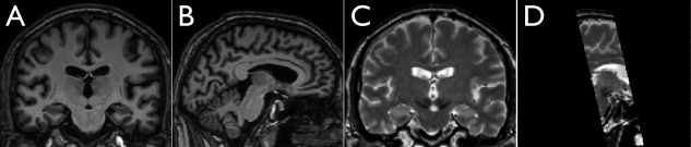
Examples of T1w and T2w MRI images from one Parkinson's disease patient in the study. From left to right: A. a coronal slice of T1w MRI cutting through the region of the red nucleus and substantia nigra; B. a sagittal slice of T1w MRI cutting through the region of the red nucleus and substantia nigra; C. a coronal slice of T2w MRI corresponding to A; and D. a sagittal section of the T2w MRI corresponding to B. Note that the T2w acquisition does not cover the entire brain.

Automatic Segmentation

In earlier investigations [Ashkan et al., 2007; Daniluk et al. 2010; Richter et al., 2004] structure identification was conducted with manual contour drawing or landmark picking (e.g., selecting the most anterior point of a structure) in the axial slices, and no volumetric segmentation or evaluation was involved. Manual segmentation can be good to identify structures, but automatic segmentation can provide more consistent results against inter‐ and intra‐rater segmentation quality incoherence while saving both labor and time. Previously, automatic segmentation techniques have contributed to morphometric studies relating to neurological diseases and brain development [Hu et al., 2013; Morra et al., 2009]. Among the proposed methods, label‐fusion techniques have gained the popularity with the robust performance in identifying structures that are typically difficult to segment solely by image intensity features. In this article, we employed the majority‐voting label‐fusion method [Aljabar et al., 2009; Heckemann et al., 2006; Rohlfing et al., 2004; Rohlfing and Maurer, 2007] to segment the RN, SN, and STN. Before segmentation, the T1w and T2w images were pre‐processed for all patients. All images were first denoised by the nonlocal mean filter technique proposed by Coupe et al. [2008], and then corrected for field inhomogeneity [Sled et al., 1998]. Each patient's T1w and T2w MRIs were rigidly coregistered using a normalized mutual information objective function [Studholme et al., 1999]. The essence of label‐fusion is to deform multiple atlases (segmented labels and MRI volumes) to the target subject's anatomy and determine the final segmentation based on the consensus of all customized atlases in order to mitigate imperfect registration and label interpolation in the single atlas deformation. In this project, 10 out of the total of 33 subjects were selected to form the label‐fusion atlas library, where each subject's brain was brought to the MNI305 space by a 9‐parameter linear registration. Then, for each subject, the SN, RN and STN were segmented manually in the stereotactic space in both hemispheres with ITK‐SNAP (http://www.itksnap.org) by an experienced neurosurgeon (CH). To further enrich the library, left‐right mirrored versions of these atlases were also included, effectively doubling the original library size.

For each subject to be segmented, the library atlases were first registered to the target patient's anatomy with a global affine registration using T1w MRI, and then deformed through local T2‐T2 nonlinear registration with SyN [Avants et al., 2008] in the central region of the brain. Here, instead of using the conventional nearest‐neighborhood interpolation, we used tri‐linear interpolation to deform the labels. This adds certain level of fuzziness to the atlases. The procedure is repeated for all 20 atlases in the template library. A demonstration of the label fusion procedure is shown in Figure 2.

Figure 2.

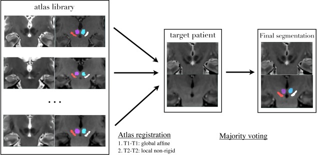
Demonstration of majority‐voting label‐fusion procedure for a Parkinson's disease patient, whose brain MRIs are in the “AC‐PC normalized space.”

To obtain the final segmentation at each voxel location in the patient's image, the structural label with the maximum counts determined voxel's label (i.e., a simple voting scheme). Some subjects from the cohort of 33 patients formed the atlas library. In these cases, the label‐fusion segmentation was performed in a leave‐one‐out manner, where the effective library would exclude the subject to be segmented.

Validation of Automatic Segmentation

The automatic label‐fusion segmentation method used to delineate the RN, SN, and STN was validated in a leave‐one‐out manner using the 10 patients' MRIs, which formed the atlas library. To avoid resampling errors and ensure the quality of comparison, the RN, SN, and STN were automatically segmented in the stereotactic space (MNI305) transformed volumes, where manual segmentations were performed. The comparison between the automatic and manual segmentation was performed with three metrics: (1) Dice overlap coefficient, or kappa = 2*a/(b + c) where a is the volume of the intersection of two segmentations, and b and c are volumes of each segmentation; (2) 95% Hausdorff distance, and (3) Euclidean distance between the centers of mass (COM) of the manual and automatic segmentations.

Coordinate Spaces

Any variability estimated will depend on the choice of coordinate space. Hence, selecting a coordinate space is important for understanding the anatomical variability and its potential link to other factors, such as the clinical information. In stereotactic neurosurgeries, the commissure points were frequently employed as the landmarks to infer the location of the subcortical structures, and thus these landmarks are natural choices to define a coordinate space to evaluate variability. To verify the spatial relationship and size differences between the nuclei and the Talairach atlas, which is often employed in the conventional DBS planning, we analyzed the variability in two different AC‐PC aligned spaces. For both spaces, AC and PC points were manually identified for each subject, and the brain was reoriented in the same manner as specified in the Talairach atlas [Talairach and Tournoux, 1988]. That is to say that the superior edge of AC and the inferior edge of PC were aligned at the centerline of the same axial plane, perpendicular to the mid‐sagittal plane of the subject's brain.

For the first space, the brain reorientation employed a rigid transformation. For the second space, in addition to the rigid transformation, all brains were scaled uniformly in three dimensions so that all AC‐PC distances were normalized to be 23 mm as measured in the Talairach atlas [Talairach and Tournoux, 1988], and the AC‐PC lines were aligned at exactly the same location for all patients. To avoid confusion, here we refer to the first and second space as the “AC‐PC native space” and “AC‐PC normalized space”, respectively. Automatic segmentations were performed for each patient in these two spaces separately. Although we mainly employed the “AC‐PC normalized space” to analyze the position and size variability, it is still important to acquire the nuclei sizes in the “AC‐PC native space” in the absence of the scaling factor for comparison. Therefore, both of them were necessary for this study.

Distance‐Based Variability Analysis

As used in many clinical papers [Ashkan et al., 2007; Daniluk et al., 2010; Richter et al., 2004], measuring Euclidean distances between points within the structure of interest and other anatomical landmarks is a straightforward approach to explore the anatomical variability in terms of both position and size. For both coordinate spaces, we measured nuclei sizes in term of volume (in mm³) as well as the extents of their 3D dimensions defined by the smallest rectangular box that contains the nucleus. The position variability of the nuclei was explored only in the “AC‐PC normalized space.” Because in DBS planning, the position of the STN is often inferred from the MC point, we measured the relative position between the center of mass (COM) of the nuclei and the geometric center of the “bounding box” to the MC point. The measurements were compared against the Talairach atlas [Talairach and Tournoux, 1988], and the comparison was studied with one‐tailed one‐sample t tests.

PCA‐Based Variability Analysis

Although the distance measurements offer quantitative comparison between subjects and standard atlases, the interpretation is less intuitive for 3D volumes. Alternatively, more detailed and intuitive morphometric variability analysis for the nuclei can be achieved using PCA, which is able to isolate shape variations that are independent in a high‐dimensional space and offers the possibility to rank them according to their level of contribution to the overall variability. To bridge the volumetric segmentation and PCA, we employed the concept of a level‐set [Osher and Sethian, 1988]. Thus, for each structure, a signed distance transformation function (negative inside, positive outside and zero at the boundary) is computed, and is served as the input for PCA. An example of the distance transformation is demonstrated for the left red nucleus with a coronal view in Figure 3. As a result, the analysis is based on continuous‐valued fields instead of landmark points identified on the surface of the 3D segmentation. The application of level‐set functions has the advantage of obviating the need to identify corresponding landmark points in the same structure of different subjects, which is very difficult for small structures.

Figure 3.

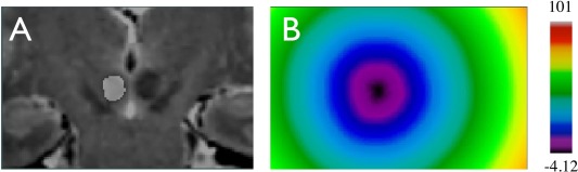
Structural segmentation and distance transformation. A. segmentation of the left red nucleus overlaid on the coronal slice of the T2w MRI; B. distance transformation of the left red nucleus label with the color map shown on the right. [Color figure can be viewed in the online issue, which is available at http://wileyonlinelibrary.com.]

Therefore, for a dataset of N patients, the distance transform function of patient i and structure L is denoted as ${\varphi }_{i,L}$, where i = {1,2, ., N} and L = {Left RN, Right RN, Left STN, Right STN, Left SN, Right SN}. Given the average level set function ${\overline{\varphi }}_L=\frac{1}{N}{\displaystyle \sum }_i{\varphi }_{i,L}$, eigenvalues ${\left\{{\lambda }_{j,L }\right\}}_{j=1,2,\mathrm{..},M}$ and the corresponding orthonormal eigenvectors (or principal components) ${\left\{P_{j,L}\right\}}_{j=1,2,\dots ,M}$ are found for the matrix $K=\frac{1}{N-1}{\mathit{S}}_{\mathit{L}}{\mathit{S}}_{\mathit{L}}^{\mathit{T}}$, where ${\mathit{S}}_{\mathit{L}}=[{\varphi }_{\sim 1,L},{\varphi }_{\sim 2,L},\dots ,{\varphi }_{\sim N,L}]$ and ${\varphi }_{\sim i,L}={\varphi }_{i,L}-{\stackrel{\sim }{\varphi }}_L$. This is achieved by decomposing K so that $K=U\Lambda U^T$ with $\Lambda$ being the diagonal matrix containing the eigenvalues and U being the orthonormal matrix that has the corresponding eigenvectors. Note that here, the eigenvectors ${\left\{{\lambda }_{j }\right\}}_{j=1,2,\mathrm{..},M}$ are arranged in the descending order.

Given a shape ψ_L, it can be represented as a linear combination of PCA components, as

$${\psi }_L={\overline{\varphi }}_L+{\displaystyle \sum }_j{w}_{j,L}{P}_{j,L}$$

where ${\overline{\varphi }}_L$ is the mean level‐set function, $P_{j,L}$ is the principal components, and $w_{j,L}=P_{j,L}\cdot {\psi }_L$ is the reconstruction coefficient of $P_{j,L}$. By changing the principal components and their associated reconstruction coefficients, different variants of the structural shapes can be obtained. Two perspectives were explored with PCA in the “AC‐PC normalized space.” First, the specific variation type with respect to each principal component (or variation mode in the context of shape analysis) was examined. This is achieved by acquiring the level set function ${\overline{\varphi }}_L\pm 3\sqrt{{\lambda }_{j,L }}{P}_{j,L}$, which represents the positive (and negative) 3‐fold standard deviation for the shape variation of the jth variation mode $P_{j,L}$. The specific type of shape variation is visually identified by comparing the binary shapes obtained by thresholding the level‐set function ${\overline{\varphi }}_L+3\sqrt{{\lambda }_{j,L }}{P}_{j,L}$ and ${\overline{\varphi }}_L-3\sqrt{{\lambda }_{j,L }}{P}_{j,L}$ with the value of 0.8. Second, the relationship between the variation modes (in the form of level‐set) and the disease progression was experimentally explored. Here, the Pearson correlation between the reconstruction coefficient $w_{j,L}$ of the jth variation mode $P_{j,L}$ and the UPDRS‐III scores while controlling for sex and age was computed for each structure under study, and the results with statistical significance (P < 0.05) were reported.

RESULTS

Automatic Segmentation and Validation

The automatic segmentations for the SN, RN and STN for one patient registered to the MNI305 space are shown in Figure 4, along with the manual segmentations in the corresponding views.

Figure 4.

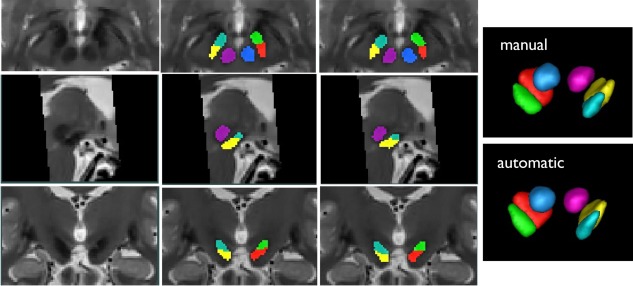
Demonstration of automatic segmentation results with one PD subject in MNI305 space. First column (from top to bottom): T2w MRI slices of the subject in axial, sagittal and coronal views; Second column: automatic segmentation results in the corresponding view of the first column; Third column: manual segmentation results in the corresponding view of the first column; Fourth column: 3D volumetric rendering of manual and automatic segmentation. Here the label colors are shown as: cyan = left STN, green = right STN, yellow = left SN, red = right SN, purple = left RN, and blue = right RN.

The segmentation validation results are shown in Figure 5 for all three evaluation metrics as boxplots with the mean values and standard deviations in the same graphs.

Figure 5.

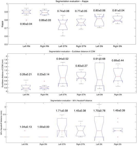
Results of automatic segmentation validation as boxplots. From top to bottom: kappa overlap coefficient, Euclidean distance between center of mass (COM), and 95% Hausdorff distance. The value of mean ± standard deviation for each result is shown beside the corresponding boxplot. [Color figure can be viewed in the online issue, which is available at http://wileyonlinelibrary.com.]

Distance‐Based Variability Analysis

The AC‐PC distance is an important measurement for the application of Talairach atlas. In the “AC‐PC native space,” the AC‐PC distance (mean ± standard deviation) is measured at 24.18 ± 1.81 mm with a range of 21.52–28.32 mm. In the Talairach atlas, the AC‐PC distance is 23 mm, which is at the 27% percentile of the cohort under study.

With a fairly large variability in the AC‐PC distance, fitting of the atlas often employs the process of scaling the AC‐PC line so that the commissures will overlap those of the patient. In this context, variability was examined in the “AC‐PC normalized space.” In general, two main factors are often investigated for the anatomical variability, size, and position. With regard to the nucleus size, we first took the measurement in terms of the medio‐lateral (M‐L), antero‐posterior (A‐P), and supero‐inferior (S‐I) dimensions of a smallest rectangular bounding box that completely contains the nucleus. The 3D dimensions of the bounding boxes were measured in both “AC‐PC native space” and “AC‐PC normalized space.” To take advantage of the volumetric segmentation, we also measured the volumes of the nuclei in mm³. Unfortunately, it was not possible to compare this value to a corresponding metric from the Talairach atlas. Both of the size measurements are detailed in Table 1, along with the corresponding available metrics obtained from the Talairach atlas.

Table 1.

Measurements of nuclei sizes as maximum extents in the medio‐lateral, antero‐posterior and supero‐inferior dimensions, as well as the nuclei volumes measured in mm³

Nucleus	Medio‐lateral (mm)	Antero‐posterior (mm)	Supero‐inferior (mm)	Size (mm3)
Left RN	6.91 ± 0.77 (7.5)	8.30 ± 0.73 (8.0)	6.79 ± 0.65 (8.5)	203.36 ± 25.75
	6.53 ± 0.53 (7.5)	8.00 ± 0. 5 6 (8.0)	6.53 ± 0.72 (8.5)	176.94 ± 32.13
Right RN	6.88 ± 0.65 (7.5)	8.24 ± 0.61 (8.0)	6.79 ± 0.60 (8.5)	203.45 ± 26.18
	6.62 ± 0.6 0 (7.5)	8.03 ± 0.62 (8.0)	6.47 ± 0.61 (8.5)	177.05 ± 31.54
Left STN	9.00 ± 0.87 (9.0)	9.70 ± 0.73 (8.5)	6.82 ± 0.85 (5.5)	156.36 ± 20.66
	8.68 ± 0.82 (9.0)	9.52 ± 0.87 (8.5)	6.44 ± 0.75 (5.5)	136.52 ± 26.23
Right STN	9.09 ± 0.88 (9.0)	9.55 ± 0.75 (8.5)	6.64 ± 0.74 (5.5)	155.73 ± 21.72
	8.67 ± 0.75 (9.0)	9.20 ± 0.7 0 (8.5)	6.35 ± 0 . 74 (5.5)	135.68 ± 29.32
Left SN	10.85 ± 0.94 (12.0)	12.73 ± 0.84 (13.0)	8.09 ± 0.98 (9.5)	285.33 ± 32.68
	10.42 ± 0.94 (12.0)	12.44 ± 0.99 (13.0)	7.85 ± 0.96 (9.5)	250.36 ± 46.00
Right SN	10.88 ± 1.17 (12.0)	12.76 ± 0.87 (13.0)	8.21 ± 0.78 (9.5)	285.52 ± 32.21
	10.32 ± 0.96 (12.0)	12.52 ± 0.89 (13.0)	7.94 ± 1.00 (9.5)	248.57 ± 46.27

Note that each value is shown as mean ± standard deviation. Here, the measurements in “AC‐PC native space” are shown in black fonts while those in “AC‐PC normalized space” are shown in bold italic fonts with underlines. The measurements from the Talairach atlas are listed in the parentheses.

From Table 1, it is shown that the mean nuclei sizes are smaller in the “AC‐PC normalized space” than the “AC‐PC native space” due to the AC‐PC distance normalization. Except the medio‐lateral dimension, the STN sizes measured from the Talairach atlas are on average smaller than the cohort in both coordinate spaces. Through t tests, we found that the sizes of the nuclei are significantly different from those in the Talairach atlas (except the A‐P dimensions of the left and right RN in the “AC‐PC normalized space,” the M‐L dimension of the left and right STN in the “AC‐PC native space,” and the A‐P dimension of the right SN in the “AC‐PC native space”).

The second main factor of anatomical variability is position. To study the position variability, the analysis was only conducted in “AC‐PC normalized space.” Because in DBS planning, the MC point is often used to infer the location of the STN, the distances between the nuclei's center of mass (COM) and the MC point in the M‐L, A‐P, and S‐I directions are reported in Table 2. Here, we see that on average, the left STN is 10.08 mm lateral, 0.94 mm posterior, and 5.00 mm inferior to the MC point while the right STN is 10.18 mm lateral, 0.71 mm posterior, and 5.06 mm inferior to the MC point. However, the center of the STN is 12 mm lateral, 2 mm posterior, and 4 mm inferior to the MC point on the Talairach atlas [Ashkan et al., 2007]. Our measurements do not correspond with those from the standard atlas, and the average STN position is more medial, more anterior, and more inferior to that in the Talairach atlas. While the previous reports [Ashkan et al., 2007; Daniluk et al., 2010] also attempt to utilize the estimated COM to measure the relative distances between the nuclei and the MC point, it is possible that this disagreement may be due to the fact that the COM of the nucleus is difficult to estimate on the 2D atlas. For the same reason, our measurements of the other nuclei locations in terms of the COM relative to the MC point were not compared with the atlas. Instead, we measured the location for geometric center of the “bounding box” of each nucleus relative to the MC point, which is more easily quantified objectively. From Table 3, it is demonstrated that such definition for the position of the STN is again significantly different (P < 0.05) between the cohort and the Talairach atlas.

Table 2.

Measured distances (mean ± standard deviation) between the COM of the nuclei and the middle commissure point in the medial‐lateral, anterior‐posterior, and superior‐inferior directions

Nucleus	Lateral to MC (mm)	Posterior to MC (mm)	Inferior to MC (mm)
Left RN	4.88 ± 0.51	7.38 ± 1.05	4.90 ± 0.75
Right RN	4.93 ± 0.53	7.24 ± 0.94	4.86 ± 0.77
Left STN	10.08 ± 1.04	0.94 ± 1.02	5.00 ± 0.89
Right STN	10.18 ± 1.00	0.71 ± 0.94	5.06 ± 0.93
Left SN	8.89 ± 0.87	4.90 ± 1.29	8.48 ± 1.00
Right SN	8.91 ± 0.79	4.86 ± 1.15	8.46 ± 1.10

Table 3.

Measured distances (mean ± standard deviation) between the geometry centers of the nuclei and the middle commissure point in the medial‐lateral, anterior‐posterior, and superior‐inferior directions

Nucleus	Lateral to MC (mm)	Posterior to MC (mm)	Inferior to MC (mm)
Left RN	4.85 ± 0.51 (4.75)	7.30 ± 1.09 (7.5)	4.95 ± 0.78 (5.25)*
Right RN	4.92 ± 0.55 (4.75)*	7.17 ± 0.92 (7.5)*	4.92 ± 0.77 (5.25)*
Left STN	9.80 ± 1.01 (9.50)	2.14 ± 1.10 (1.25)*	4.97 ± 1.01 (3.75)*
Right STN	9.83 ± 0.96 (9.50)*	1.96 ± 1.05 (1.25)*	4.97 ± 0.92 (3.75)*
Left SN	9.16 ± 0.89 (9.00)	4.83 ± 1.36 (6.00)*	7.57 ± 0.88 (8.25)*
Right SN	9.12 ± 0.79 (9.00)	4.70 ± 1.29 (6.00)*	7.67 ± 1.03 (8.25)*

An asterisk (“*”) indicates that the measurement disagrees with that from the Talairach atlas with statistical significance (P < 0.05).

PCA‐Based Variability Analysis

The experiments above give an idea of the positions and extents of the STN, RN and SN, but don't give any insight into how the shapes of these structures vary in the PD population. To address this limitation, PCA analysis was performed in “AC‐PC normalized space” for each structure with the left and right side analyzed separately. The PCA analysis decomposes the anatomical variability into ranked variation modes, and thus allows a more intuitive view on the nature of the variability. For all structures of interest, the first 5 and the first 10 components account for 95–98% and roughly 99% of the total variability, respectively. The eigenvalues of the first 10 components for all structures are illustrated as bar plots in Figure 6.

Figure 6.

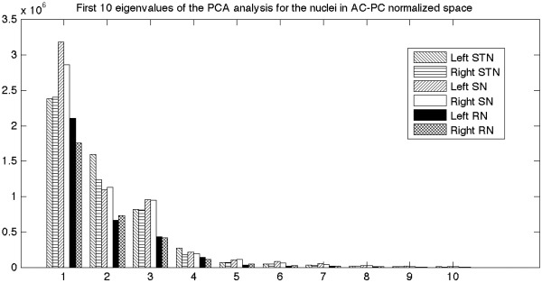
Bar plot showing the eigenvalues of the first 10 principal components from the PCA analysis of each nucleus.

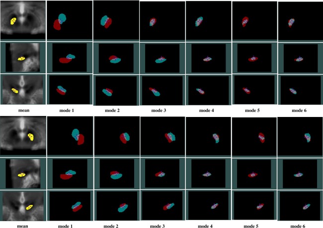
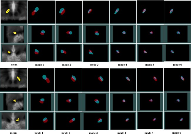
Through investigating the ordered eigenvalues of the structures using one‐tailed paired sample t tests, the eigenvalues of the RN are significantly lower (P < 0.05) than those of the SN and STN on the respective side. This implies that in terms of variability, the RN is less variable than the SN and STN. To demonstrate the variation modes, the first six most prominent shape variations for all structures are shown from Figure 7, 8 to 9, with the degree of threefold standard deviation (negative and positive) from the mean shape. Through the evolution between the two extreme shape variations (negative and positive deviations) for each mode, we can identify the specific type of shape variation that is represented by a mode. In the same figures, the mean shapes are overlaid on the average of all 33 AC‐PC normalized T2w MRIs, and they, not surprisingly, fit the averaged T2w MRI after AC‐PC normalization. However, owing to the structural variability remaining after the linear AC‐PC scaling alignment, the nuclei in the averaged T2w MRI appear blurry.

Figure 7.

PCA analysis results for the left (top three rows) and right (bottom three rows) RN showing effects of the first six variation modes and the mean shape overlaid on an average of AC‐PC normalized T2w MRIs. For each variation mode shown, the cyan color label represents mean shape minus threefold standard deviation while the red color label represents mean shape plus threefold standard deviation. Note that in each group of figures demonstrating the left or right RN, the cross‐hair cursor is placed at the same position, and the three rows show the axial, sagittal, and coronal views (from top to bottom) of the nucleus.

Figure 8.

PCA analysis results for the left (top three rows) and right (bottom three rows) SN showing effects of the first six variation modes and the mean shape overlaid on an average of AC‐PC normalized T2w MRIs. For each variation mode shown, the cyan color label represents mean shape minus threefold standard deviation while the red color label represents mean shape plus threefold standard deviation. Note that in each group of figures demonstrating the left or right SN, the cross‐hair cursor is placed at the same position, and the three rows show the axial, sagittal, and coronal views (from top to bottom) of the nucleus.

Figure 9.

PCA analysis results for the left (top three rows) and right (bottom three rows) STN showing effects of the first 6 variation modes and the mean shape overlaid on an average of AC‐PC normalized T2w MRIs. For each variation mode shown, the cyan color label represents mean shape minus threefold standard deviation while the red color label represents mean shape plus threefold standard deviation. Note that in each group of figures demonstrating the left or right STN, the cross‐hair cursor is placed at the same position, and the three rows show the axial, sagittal, and coronal views (from top to bottom) of the nucleus.

In general, for each structure, the first three shape variations are mostly related to the spatial displacements while the later principal components account for relatively more subtle global and local shape variations. More specifically, for the RN, the A‐P position displacement appears most significant, and the M‐L and S‐I displacements are secondary. It is interesting that for the RN, the second and third mode appear very similar in nature, but the direction of the displacement in space varies. For the SN and STN, a mix of A‐P and S‐I position difference is the most dominant. However, for the SN, the importance of S‐I and M‐L displacements come in the second and third while for the STN, after the first mode, the contribution of the M‐L displacement is more than the S‐I displacement. Overall, within the principal component representation of the position variability, the variability often involves displacements in three principal directions (medio‐lateral, infero‐superior, and antero‐posterior), but a prevailing trend in one or two directions can still be easily identified.

An additional observation is that while on average the variation modes appear similar between the left and right side, the symmetry does not hold all the time. Example of this phenomenon can be seen when comparing bilaterally the third modes of the SN and STN, as well as in the later principal component representations. Despite the symmetry assumption in many atlases, it is not surprising to discover asymmetric anatomical variability in these nuclei as in many other structures in the human brain.

Correlation

To explore the influence of the disease over the variations revealed by PCA analysis, we computed the Pearson correlation between the reconstruction coefficients for each variation mode and the clinical information (on‐Dopa and off‐Dopa UPDRS III) of the patients while controlling for age and sex. Given the exploratory nature of this analysis, the partial correlations with a significant level (P < 0.05), uncorrected for multiple comparisons, are shown in Table 4. It is mentioned earlier that for all structures of interest, the first 10 variation modes account for about 99% of the observed variation. Therefore, to avoid noise that may mislead the interpretation, the correlations are only listed for the relevant first 10 variation modes in Table 4. The variation modes showing significant correlations are different between the case of on‐ and off‐Dopa UPDRS III scores, and furthermore, the examination results are not symmetric between the left and right side. More specifically, as the on‐Dopa UPDRS III score increases, the positions of the right RN (Mode 3), right STN (Mode 2), and right SN (Mode 3) become more lateral, and the superior portion of the right RN is reduced (Mode 4). As of the off‐Dopa UPDRS III scores, with higher scores, the right STN is more infero‐posterior (Mode 1), the left STN size is smaller (Mode 7), and the right RN is more posterior (Mode 1).

Table 4.

Table of variation modes that have statistically significant (P < 0.05) correlations with on‐ and off‐Dopa UPDRS III scores

Nucleus	On‐Dopa UPDRS III		Off‐Dopa UPDRS III
Left RN
Right RN	Mode 3 (0.35)	Mode 4 (0.55)	Mode 1 (0.34)
Left STN			Mode 7 (0.45)
Right STN	Mode 2 (0.43)		Mode 1 (0.36)
Left SN
Right SN	Mode 3 (0.38)

Note that the value of correlation is shown inside the parenthesis after the respective variation mode number. Here, only the first 10 variation modes are shown in the table.

DISCUSSION

Label Fusion

For the purpose of nuclei segmentation, we employed the majority‐voting label‐fusion technique despite that a number of more recent and sophisticated label‐fusion techniques [Artaechevarria et al., 2009; Chen et al., 2012; Coupe et al., 2011; Isgum et al., 2009; Wang et al., 2011, 2013; Warfield et al., 2004] have demonstrated superior performance by exploring statistical behaviors of the images and atlases. Two reasons contribute to our selection of segmentation method. First, the relatively simple majority‐voting segmentation has shown robust performance [Aljabar et al., 2009; Collins and Pruessner, 2010; Heckemann et al., 2006; Rohlfing et al., 2004; Rohlfing and Maurer, 2007]. Second, a complete comparison of these new methods is not available, and the performance of the more sophisticated segmentation techniques depends on successful reimplementation. It is true that majority‐voting label‐fusion techniques have never been used in segmenting midbrain nuclei. However, a comparison of different algorithms is beyond the scope of this article. By visual inspection, the selected segmentation method demonstrates satisfactory results according to the manual segmentation protocols adopted by the neurosurgeon who labeled the relevant structures for the atlas library. From quantitative validation, we have achieved fairly satisfactory results for such small structures, compared with previous publications in terms of kappa [Haegelen et al., 2012] and the Euclidean distance between COMs [Brunenberg et al., 2011]. In this study, to further ensure the segmentation accuracy, T2‐T2 nonlinear registration was used instead of the more common T1‐T1 registration seen in DBS applications.

Stereotactic Spaces

The selection of coordinate space affects the final results of the morphological study. In an ideal mathematical analysis, one would identify the minimum variance frame [Bookstein, 1977] of selected landmarks, and report variability within this coordinate system. However, our goal was to identify anatomical variability in a coordinate system that is commonly used in stereotaxic neurosurgery. While it is true that the use of an AC‐PC based coordinate system mixes displacement and shape information, it is precisely the result of this mixing that is required by the neurosurgeons when determining optimal targets for deep brain surgery. While both are employed in DBS planning, the Schaltenbrand atlas [Schaltenbrand and Wahren, 1977] is more commonly seen in the previous studies of midbrain nuclei anatomical variability [Ashkan et al., 2007; Castro et al., 2006; Daniluk et al., 2010; Richter et al., 2004] than the Talairach atlas [Talairach and Tournoux, 1988]. However, we referred to the latter for our analysis. In contrast to the Talairach atlas, which only contains one healthy aged female subject without Parkinson's disease, the Schaltenbrand atlas was created with different subjects for different sections. To obtain more consistent dimension measurements, the Talairach atlas may be a better choice. However, the locations of the RN, SN and STN in the Talairach atlas do not represent the mean coordinates of a population since it was derived from the anatomy of a single individual, and these coordinates are different from the mean coordinates found in our study. Furthermore, the definitions of AC‐PC line and thus the MC point in these two atlases differ [Weiss et al., 2003], making it difficult to simultaneously compare the two atlases to the measurements of the cohort in the same coordinate space. Besides the histology‐derived stereotactic spaces, there also exist MRI‐derived stereotactic spaces, such as the ICBM152 [Fonov et al., 2011] and MNI305 spaces [Collins et al., 1994]. These newer stereotactic spaces resemble the brain orientation of the Talairach space, and the stereotactic space realignment for any upcoming subject is achieved fully automatically. Variability analysis [Forstmann et al., 2012] has also been previously conducted using such stereotactic space. Yet, often due to the availability of the software and the long history of successful applications in neurological studies, the histology‐derived atlases [Schaltenbrand and Wahren, 1977; Talairach and Tournoux, 1988] are still more commonly employed.

Morphometric Variability

While T2w MRI is still the most common way to image the midbrain nuclei in the clinics, as the medical imaging technology advances, there have been a number of MRI methods [Brunenberg et al., 2011; O'Gorman et al., 2011; Xiao et al., 2012] designed to directly visualize the STN. Consequently, this raised the debate of whether direct targeting using these MRI methods is superior to the classical landmark‐based indirect targeting method. On one hand, some studies [Richter et al., 2004; Zhu et al., 2002] support the use of direct visualization; on the other hand, a number of studies [Acar et al., 2007; Guehl et al., 2007; Lanotte et al., 2002; McClelland et al., 2005] have reported successful application of indirect targeting. As a result, an investigation is still necessary, especially with better imaging methods and high field scanners becoming increasingly available.

Similar to a previous study [Richter et al., 2004], the measured STN size is smaller than or similar to that of the Talairach atlas [Talairach and Tournoux, 1988] in the M‐L dimension, but larger in the I‐S and A‐P dimensions. We find the geometric center of the STN is more posterior, lateral and inferior to that in the Talairach atlas. This confirms the study by Richter et al. [2004]. Unfortunately, most previous studies only focused on the analysis of the STN, and their AC‐PC line alignment may differ from the method described in this article, especially when using the Schaltenbrand atlas [Schaltenbrand and Wahren, 1977] as the reference. It is difficult to compare our results, and especially those of the RN and SN, to previous publications. Nevertheless, the additional measurements of the RN and SN, and the comparison to the Talairach atlas with a larger population than in [Richter et al., 2004] provide valuable complementary knowledge to the application of atlases.

As far as the cohort is concerned, the Talairach atlas [Talairach and Tournoux, 1988] does not match our measurements. One possible reason for the disagreement is that the subject for atlasing lacks of sufficient representativeness of the population under study (i.e., PD). This is a universal issue for all single‐subject derived atlases. In this sense, unbiased anatomical atlases [Fonov et al., 2011; Haegelen et al., 2012] that represent the averaged anatomical features of the population of interest (i.e., advanced PD patients) may be more desirable as both aging and disease progression may alter the anatomy due to global and local tissue degeneration and atrophy. Whether targeting the STN with such unbiased atlas is superior than direct visualization will require further evaluation beyond the scope of this article. At the moment, the evidence presented here supports the use of direct targeting method over the landmark‐based indirect targeting based on the Talairach atlas.

Another issue related to the analysis is image distortion. For the image protocols involved, a distortion study was conducted using a LEGO phantom, and the procedure is detailed in [Caramanos et al., 2010]. Through the analysis, an average distortion below 0.5 mm was measured within the field of view for both T1w and T2w MRI protocols presented. For the central region, where our analysis was conducted, the distortion is close to 0.2 mm. Compared with the magnitude of our measurements, this will not likely influence our final conclusion that the metrics obtained from the cohort differ from the Talairach atlas.

In this study, PCA offers a new perspective on the issue of anatomical variability of the midbrain nuclei compared with the conventional coordinate analysis. When correlated with clinical information (UPDRS III scores) in our exploratory analysis, one can identify specific types of shape variation that are possibly related to the disease progression. In addition, the intuitive nature of the analysis results allows visual identification of the subtle morphometric changes possibly due to disease progression. With the help of PCA, we discovered the lateral displacement of the nuclei with disease progression on the right side likely due to the enlargement of the third ventricle [Daniluk et al., 2010], but the asymmetry of this discovery requires further investigation. The off‐Dopa UPDRS III scores were shown to be related to the STN with size reduction on the left side and position alteration on the right side, as well as position shift of the right RN. The difference between the on‐ and off‐Dopa results is very likely due to the interplay between the structure changes and the influence of external dopamine supply. It should also be noted that the morphometric alterations of the nucleus for PD should be a result of shape changes of both the nucleus itself and the surrounding structures (i.e. ventricle enlargement and brain atrophy). The PCA exploratory analysis may offer a potential method for disease prediction of Parkinson's disease. However, it is important to note two important limitations of our study: First, we have reported preliminary results on only 33 subjects: more subjects are needed to confirm the results and to expand the analysis. Second, we have reported significant correlations with uncorrected P values to identify potential relations between shape and disease progression. Given the large number of correlations computed, some of these results may be due to chance. To better understand and further confirm these correlations, a larger patient population is required. For this study, only the motor‐function‐related UPDRS III scores were used because among all the UPDRS assessment subscores, this metric is obtained most objectively by the neurologist while the rest were self‐evaluated by the patients, and the motor function disability is more prominent than other cognitive and psychological symptoms for PD.

CONCLUSION

In conclusion, we analyzed the sizes and positions of the STN and the adjacent RN and SN by using the label‐fusion technique to automatically segment structures from high resolution 3 Tesla TSE T2w MRIs. From the analysis, significant differences were discovered between the studied cohort and the Talairach atlas, and the discovery supports the use of MRI‐based direct targeting method for locating the SN, RN, and STN. In addition to conventional coordinate measurement, we employed PCA analysis to obtain more intuitive and detailed information regarding the morphometric variability of the nuclei, and correlations between the PCA components and UPDRS III scores were found.

REFERENCES

- Acar F, Miller JP, Berk MC, Anderson G, Burchiel KJ (2007): Safety of anterior commissure‐posterior commissure‐based target calculation of the subthalamic nucleus in functional stereotactic procedures. Stereotact Funct Neurosurg 85:287–291. [DOI] [PubMed] [Google Scholar]
- Aljabar P, Heckemann RA, Hammers A, Hajnal JV, Rueckert D (2009): Multi‐atlas based segmentation of brain images: Atlas selection and its effect on accuracy. Neuroimage 46:726–738. [DOI] [PubMed] [Google Scholar]
- Artaechevarria X, Munoz‐Barrutia A, Ortiz‐de‐Solorzano C (2009): Combination strategies in multi‐atlas image segmentation: Application to brain MR data. IEEE Trans Med Imaging 28:1266–1277. [DOI] [PubMed] [Google Scholar]
- Ashkan K, Blomstedt P, Zrinzo L, Tisch S, Yousry T, Limousin‐Dowsey P, Hariz MI (2007): Variability of the subthalamic nucleus: The case for direct MRI guided targeting. Br J Neurosurg 21:197–200. [DOI] [PubMed] [Google Scholar]
- Avants BB, Epstein CL, Grossman M, Gee JC (2008): Symmetric diffeomorphic image registration with cross‐correlation: Evaluating automated labeling of elderly and neurodegenerative brain. Med Image Anal 12:26–41. [DOI] [PMC free article] [PubMed] [Google Scholar]
- Bookstein FL (1977): Study of shape transformation after Darcy Thompson. Math Biosci 34:177–219. [Google Scholar]
- Brunenberg EJ, Platel B, Hofman PA, Ter Haar Romeny BM, Visser‐Vandewalle V (2011): Magnetic resonance imaging techniques for visualization of the subthalamic nucleus. J Neurosurg 115:971–984. [DOI] [PubMed] [Google Scholar]
- Camicioli R, Moore MM, Kinney A, Corbridge E, Glassberg K, Kaye JA (2003): Parkinson's disease is associated with hippocampal atrophy. Movement Disord 18:784–790. [DOI] [PubMed] [Google Scholar]
- Caramanos Z, Fonov VS, Francis SJ, Narayanan S, Pike GB, Collins DL, Arnold DL (2010): Gradient distortions in MRI: Characterizing and correcting for their effects on SIENA‐generated measures of brain volume change. Neuroimage 49:1601–1611. [DOI] [PubMed] [Google Scholar]
- Castro FJ, Pollo C, Meuli R, Maeder P, Cuisenaire O, Cuadra MB, Villemure JG, Thiran JP (2006): A cross validation study of deep brain stimulation targeting: From experts to atlas‐based, segmentation‐based and automatic registration algorithms. IEEE Trans Med Imaging 25:1440–1450. [DOI] [PubMed] [Google Scholar]
- Chen A, Niermann KJ, Deeley MA, Dawant BM (2012): Evaluation of multiple‐atlas‐based strategies for segmentation of the thyroid gland in head and neck CT images for IMRT. Phys Med Biol 57:93–111. [DOI] [PMC free article] [PubMed] [Google Scholar]
- Collins DL, Pruessner JC (2010): Towards accurate, automatic segmentation of the hippocampus and amygdala from MRI by augmenting ANIMAL with a template library and label fusion. Neuroimage 52:1355–1366. [DOI] [PubMed] [Google Scholar]
- Collins DL, Neelin P, Peters TM, Evans AC (1994): Automatic 3D intersubject registration of MR volumetric data in standardized Talairach space. J Comput Assist Tomogr 18:192–205. [PubMed] [Google Scholar]
- Coupe P, Yger P, Prima S, Hellier P, Kervrann C, Barillot C (2008): An optimized blockwise nonlocal means denoising filter for 3‐D magnetic resonance images. IEEE Trans Med Imaging 27:425–441. [DOI] [PMC free article] [PubMed] [Google Scholar]
- Coupe P, Manjon JV, Fonov V, Pruessner J, Robles M, Collins DL (2011): Patch‐based segmentation using expert priors: Application to hippocampus and ventricle segmentation. Neuroimage 54:940–954. [DOI] [PubMed] [Google Scholar]
- Daniluk SKGD, Ellias SA, Novak P, Nazzaro JM (2010): Assessment of the variability in the anatomical position and size of the subthalamic nucleus among patients with advanced Parkinson's disease using magnetic resonance imaging. Acta Neurochir (Wien) 152:201–210; discussion 210. [DOI] [PubMed] [Google Scholar]
- den Dunnen WF, Staal MJ (2005): Anatomical alterations of the subthalamic nucleus in relation to age: A postmortem study. Mov Disord 20:893–898. [DOI] [PubMed] [Google Scholar]
- Fonov V, Evans AC, Botteron K, Almli CR, McKinstry RC, Collins DL (2011): Unbiased average age‐appropriate atlases for pediatric studies. Neuroimage 54:313–327. [DOI] [PMC free article] [PubMed] [Google Scholar]
- Forstmann BU, Keuken MC, Jahfari S, Bazin PL, Neumann J, Schafer A, Anwander A, Turner R (2012): Cortico‐subthalamic white matter tract strength predicts interindividual efficacy in stopping a motor response. Neuroimage 60:370–375. [DOI] [PubMed] [Google Scholar]
- Guehl D, Edwards R, Cuny E, Burbaud P, Rougier A, Modolo J, Beuter A (2007): Statistical determination of the optimal subthalamic nucleus stimulation site in patients with Parkinson disease. J Neurosurg 106:101–110. [DOI] [PubMed] [Google Scholar]
- Haegelen C, Coupe P, Fonov V, Guizard N, Jannin P, Morandi X, Collins DL (2012): Automated segmentation of basal ganglia and deep brain structures in MRI of Parkinson's disease. Int J Comput Assist Radiol Surg 8:99–110. [DOI] [PMC free article] [PubMed] [Google Scholar]
- Heckemann RA, Hajnal JV, Aljabar P, Rueckert D, Hammers A (2006): Automatic anatomical brain MRI segmentation combining label propagation and decision fusion. Neuroimage 33:115–126. [DOI] [PubMed] [Google Scholar]
- Hu S, Pruessner JC, Coupe P, Collins DL (2013): Volumetric analysis of medial temporal lobe structures in brain development from childhood to adolescence. Neuroimage 74:276–287. [DOI] [PubMed] [Google Scholar]
- Hutchinson M, Raff U (2000): Structural changes of the substantia nigra in Parkinson's disease as revealed by MR imaging. Am J Neuroradiol 21:697–701. [PMC free article] [PubMed] [Google Scholar]
- Isgum I, Staring M, Rutten A, Prokop M, Viergever MA, van Ginneken B (2009): Multi‐atlas‐based segmentation with local decision fusion—Application to cardiac and aortic segmentation in CT scans. IEEE Trans Med Imaging 28:1000–1010. [DOI] [PubMed] [Google Scholar]
- Keuken MC, Bazin PL, Schafer A, Neumann J, Turner R, Forstmann BU (2013): Ultra‐high 7T MRI of structural age‐related changes of the subthalamic nucleus. J Neurosci 33:4896–4900. [DOI] [PMC free article] [PubMed] [Google Scholar]
- Kitajima M, Korogi Y, Kakeda S, Moriya J, Ohnari N, Sato T, Hayashida Y, Hirai T, Okuda T, Yamashita Y (2008): Human subthalamic nucleus: Evaluation with high‐resolution MR imaging at 3.0 T. Neuroradiology 50:675–681. [DOI] [PubMed] [Google Scholar]
- Kleiner‐Fisman G, Fisman DN, Sime E, Saint‐Cyr JA, Lozano AM, Lang AE (2003): Long‐term follow up of bilateral deep brain stimulation of the subthalamic nucleus in patients with advanced Parkinson disease. J Neurosurg 99:489–495. [DOI] [PubMed] [Google Scholar]
- Lanotte MM, Rizzone M, Bergamasco B, Faccani G, Melcarne A, Lopiano L (2002): Deep brain stimulation of the subthalamic nucleus: Anatomical, neurophysiological, and outcome correlations with the effects of stimulation. J Neurol Neurosurg Psychiatry 72:53–58. [DOI] [PMC free article] [PubMed] [Google Scholar]
- Massey LA, Miranda MA, Zrinzo L, Al‐Helli O, Parkes HG, Thornton JS, So PW, White MJ, Mancini L, Strand C, Holton JL, Hariz MI, Lees AJ, Revesz T, Yousry TA (2012): High resolution MR anatomy of the subthalamic nucleus: Imaging at 9.4 T with histological validation. Neuroimage 59:2035–2044. [DOI] [PubMed] [Google Scholar]
- McClelland S III, Ford B, Senatus PB, Winfield LM, Du YE, Pullman SL, Yu Q, Frucht SJ, McKhann GM II, Goodman RR (2005): Subthalamic stimulation for Parkinson disease: Determination of electrode location necessary for clinical efficacy. Neurosurg Focus 19:E12. [PubMed] [Google Scholar]
- Montgomery EB (2010): Deep Brain Stimulation Programming: Principles and Practice, Vol. 17 Oxford: Oxford University Press, pp 179. [Google Scholar]
- Morra JH, Tu Z, Apostolova LG, Green AE, Avedissian C, Madsen SK, Parikshak N, Hua X, Toga AW, Jack CR Jr, Schuff N, Weiner MW, Thompson PM (2009): Automated 3D mapping of hippocampal atrophy and its clinical correlates in 400 subjects with Alzheimer's disease, mild cognitive impairment, and elderly controls. Hum Brain Mapp 30:2766–2788. [DOI] [PMC free article] [PubMed] [Google Scholar]
- Murphy DGM, Decarli C, Schapiro MB, Rapoport SI, Horwitz B (1992): Age‐related differences in volumes of subcortical nuclei, brain matter, and cerebrospinal‐fluid in healthy‐men as measured with magnetic‐resonance‐imaging. Arch Neurol‐Chicago 49:839–845. [DOI] [PubMed] [Google Scholar]
- Nagano‐Saito A, Washimi Y, Arahata Y, Kachi T, Lerch JP, Evans AC, Dagher A, Ito K (2005): Cerebral atrophy and its relation to cognitive impairment in Parkinson disease. Neurology 64:224–229. [DOI] [PubMed] [Google Scholar]
- Nowinski WL, Belov D, Pollak P, Benabid AL (2004): A probabilistic functional atlas of the human subthalamic nucleus. Neuroinformatics 2:381–398. [DOI] [PubMed] [Google Scholar]
- O'Gorman RL, Shmueli K, Ashkan K, Samuel M, Lythgoe DJ, Shahidiani A, Wastling SJ, Footman M, Selway RP, Jarosz J (2011): Optimal MRI methods for direct stereotactic targeting of the subthalamic nucleus and globus pallidus. Eur Radiol 21:130–136. [DOI] [PubMed] [Google Scholar]
- Osher S, Sethian JA (1988): Fronts propagating with curvature‐dependent speed—Algorithms based on Hamilton‐Jacobi formulations. J Comput Phys 79:12–49. [Google Scholar]
- Patel NK, Khan S, Gill SS (2008): Comparison of atlas‐ and magnetic‐resonance‐imaging‐based stereotactic targeting of the subthalamic nucleus in the surgical treatment of Parkinson's disease. Stereotact Funct Neurosurg 86:153–161. [DOI] [PubMed] [Google Scholar]
- Richter EO, Hoque T, Halliday W, Lozano AM, Saint‐Cyr JA (2004): Determining the position and size of the subthalamic nucleus based on magnetic resonance imaging results in patients with advanced Parkinson disease. J Neurosurg 100:541–546. [DOI] [PubMed] [Google Scholar]
- Rohlfing T, Maurer CR Jr (2007): Shape‐based averaging. IEEE Trans Image Process 16:153–161. [DOI] [PubMed] [Google Scholar]
- Rohlfing T, Brandt R, Menzel R, Maurer CR Jr (2004): Evaluation of atlas selection strategies for atlas‐based image segmentation with application to confocal microscopy images of bee brains. Neuroimage 21:1428–1442. [DOI] [PubMed] [Google Scholar]
- Scahill RI, Frost C, Jenkins R, Whitwell JL, Rossor MN, Fox NC (2003): A longitudinal study of brain volume changes in normal aging using serial registered magnetic resonance imaging. Arch Neurol‐Chicago 60:989–994. [DOI] [PubMed] [Google Scholar]
- Schaltenbrand G, Wahren W (1977): Atlas for Stereotaxy of the Human Brain, Vol. 13 Chicago: Year Book Medical Publishers; pp 66. [Google Scholar]
- Sled JG, Zijdenbos AP, Evans AC (1998): A nonparametric method for automatic correction of intensity nonuniformity in MRI data. IEEE Trans Med Imaging 17:87–97. [DOI] [PubMed] [Google Scholar]
- Studholme C, Hill DLG, Hawkes DJ (1999): An overlap invariant entropy measure of 3D medical image alignment. Pattern Recogn 32:71–86. [Google Scholar]
- Talairach J, Tournoux P (1988): Co‐planar Stereotaxic Atlas of the Human Brain: 3‐Dimensional Proportional System: An Approach to Cerebral Imaging, Vol. 8 New York: Thieme Medical Publishers; pp 122. [Google Scholar]
- Vingerhoets FJ, Villemure JG, Temperli P, Pollo C, Pralong E, Ghika J (2002): Subthalamic DBS replaces levodopa in Parkinson's disease: Two‐year follow‐up. Neurology 58:396–401. [DOI] [PubMed] [Google Scholar]
- Wang H, Suh JW, Pluta J, Altinay M, Yushkevich P (2011): Optimal weights for multi‐atlas label fusion. Inf Process Med Imaging 22:73–84. [DOI] [PMC free article] [PubMed] [Google Scholar]
- Wang H, Suh JW, Das SR, Pluta J, Craige C, Yushkevich PA (2013): Multi‐atlas segmentation with joint label fusion. IEEE Trans Pattern Anal Mach Intell 35:611–623. [DOI] [PMC free article] [PubMed] [Google Scholar]
- Warfield SK, Zou KH, Wells WM (2004): Simultaneous truth and performance level estimation (STAPLE): An algorithm for the validation of image segmentation. IEEE Trans Med Imaging 23:903–921. [DOI] [PMC free article] [PubMed] [Google Scholar]
- Weiss KL, Pan H, Storrs J, Strub W, Weiss JL, Jia L, Eldevik OP (2003): Clinical brain MR imaging prescriptions in Talairach space: Technologist‐ and computer‐driven methods. Am J Neuroradiol 24:922–929. [PMC free article] [PubMed] [Google Scholar]
- Xiao YM, Beriault S, Pike GB, Collins DL (2012): Multicontrast multiecho FLASH MRI for targeting the subthalamic nucleus. Magn Reson Imaging 30:627–640. [DOI] [PubMed] [Google Scholar]
- Zhu XL, Hamel W, Schrader B, Weinert D, Hedderich J, Herzog J, Volkmann J, Deuschl G, Muller D, Mehdorn HM (2002): Magnetic resonance imaging‐based morphometry and landmark correlation of basal ganglia nuclei. Acta Neurochir (Wien) 144:959–969; discussion 968–969. [DOI] [PubMed] [Google Scholar]