Abstract
This data article contains data related to the research article entitled “Global land cover classification based on microwave polarization and gradient ratio (MPGR)” [1] and “Microwave polarization and gradient ratio (MPGR) for global land surface phenology” [2]. This data article presents land surface characteristics and snow cover variation information from sensors like EOS Advanced Microwave Scanning Radiometer (AMSR-E). This data article use the HDF Explorer, Matlab, and ArcGIS software to process the pixel latitude, longitude, snow water equivalent (SWE), digital elevation model (DEM) and Brightness Temperature (BT) information from AMSR-E satellite data to provide land surface characteristics and snow cover variation data in all-weather condition at any time. This data information is useful to discriminate different land surface cover types and snow cover variation, which is turn, will help to improve monitoring of weather, climate and natural disasters.
|
Specifications Table | |
| Subject area | Earth and Space Science |
| More specific subject area | Remote Sensing, GIS and Geo-informatics |
| Type of data | Image, table, figure, graph |
| How data was acquired | Collect from Satellite Climate Studies Branch/National Oceanic and Atmospheric Administration (NOAA), and Goddard Space Flight Centre/National Aeronautics and Space Administration (NASA), and download from United States Geological Survey (USGS) website |
| Data format | Analyzed |
| Experimental factors | Image processing |
| Experimental features | Georeferenced, Change Detection, Image Enhancement, Band Combination, Resampling, Principal Component Analysis, Image Classification, Combined satellite data in GIS with the help of HDF Explorer, Matlab, ArcGIS software |
| Data source location | NOAA/NESDIS/STAR/Satellite Climate Studies Branch College Park MD, USA. Cooperative Institute for Climate and Satellites (CICS), ESSIC, University of Maryland College Park, MD, USA. Goddard Space Flight Centre NASA, Greenbelt, MD, USA |
| Data accessibility | Data is in this data article |
Value of the data
-
•
This data information is useful to understand the land surface characteristics to use in weather forecasting applications, even during cloudy and precipitation conditions which often interferes with other sensors [2], [3].
-
•
This data information is useful for timely monitoring of natural disasters for minimizing economic losses caused by floods, drought, etc. Actually access of large-scale regional land surface information is critical to emergency management during natural disasters [4], [5].
-
•
This data information helps us to understand how satellite remote sensing can be useful for the long-term observation of the intra and inter-annual variability of snow packs in rather inaccessible regions and providing useful information on a critical component of the hydrological cycle, where the network of meteorological stations is deficient [6], [7].
-
•
This data information is useful for monitoring the seasonal snow cover variation for several purposes such as climatology, hydrometeorology, water use and control and hydrology, including flood forecasting and food production [8], [9].
1. Data
The dataset of this article provide following information:
-
A.
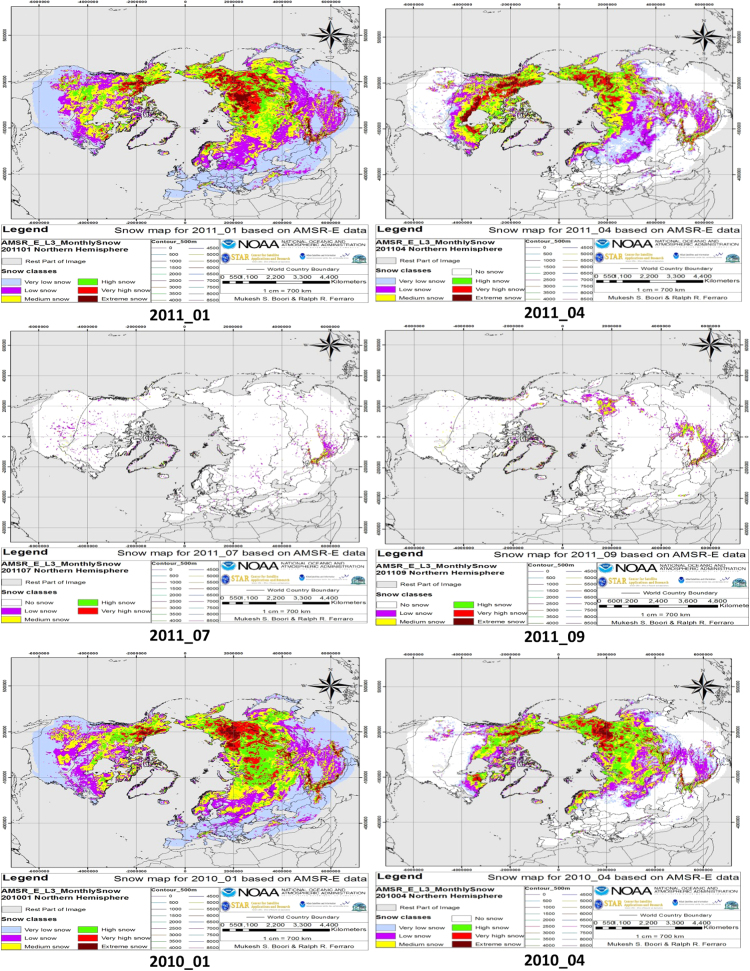
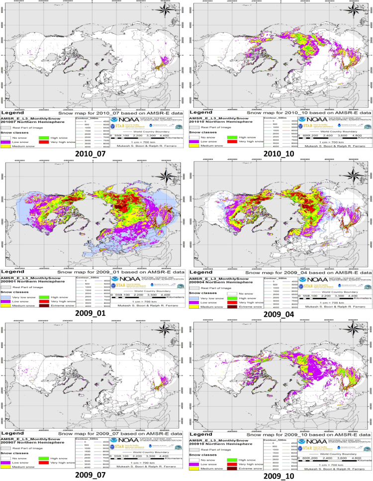
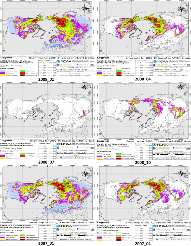
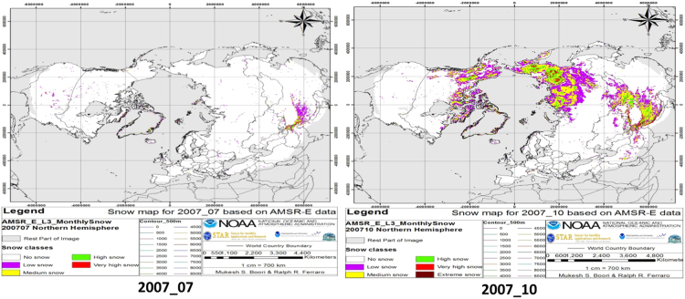
Snow cover variation with seasons and elevation (Fig. 1 and Table 1, Table 2).
-
B.
Land use/cover classified map based on MPGR values (Fig. 2 and Table 3).
-
C.
Different frequencies actual physical land surface temperature (Fig. 3).
Fig. 1.
Snow cover with snow classes from 2007 to 2011 for January, April, July, and October months.
Table 1.
Snow classes and snow cover area in million km2 for January, April, July and October months from 2007 to 2011.
| Class |
2011_01 |
2010_01 |
2009_01 |
2008_01 |
2007_01 |
||||||||||
|---|---|---|---|---|---|---|---|---|---|---|---|---|---|---|---|
| Area | % | Area | % | Area | % | Area | % | Area | % | ||||||
| Very low snow | 21.9 | 36.4 | 21.4 | 35.7 | 22.2 | 37.0 | 21.7 | 36.2 | 24.3 | 40.6 | |||||
| Low snow | 13.4 | 22.3 | 13.2 | 21.9 | 15.1 | 25.1 | 14.8 | 24.7 | 13.2 | 22.1 | |||||
| Medium snow | 11.5 | 19.1 | 11.2 | 18.7 | 11.2 | 18.7 | 11.9 | 19.9 | 11.4 | 19.0 | |||||
| High snow | 7.5 | 12.5 | 8.6 | 14.4 | 6.7 | 11.1 | 6.7 | 11.2 | 6.3 | 10.5 | |||||
| Very high snow | 4.3 | 7.2 | 4.4 | 7.3 | 3.7 | 6.1 | 3.5 | 5.8 | 3.6 | 5.9 | |||||
| Extreme snow | 1.5 | 2.5 | 1.2 | 2.0 | 1.2 | 1.9 | 1.3 | 2.2 | 1.2 | 1.9 | |||||
| Total snow | 60.0 | 100.0 | 60.0 | 100.0 | 60.0 | 100.0 | 60.0 | 100.0 | 60.0 | 100.0 | |||||
| RPI | 264.9 | 264.9 | 264.9 | 264.9 | 264.9 | ||||||||||
| Total | 324.8 | 324.8 | 324.8 | 324.8 | 324.8 | ||||||||||
|
2011_04 |
2010_04 |
2009_04 |
2008_04 |
2007_04 |
|||||||||||
| Class | Area | % | % | Area | % | % | Area | % | % | Area | % | % | Area | % | % |
| Very low snow | 10.7 | 27.8 | 17.8 | 8.6 | 24.2 | 14.3 | 8.8 | 24.3 | 14.7 | 9.5 | 26.6 | 15.9 | 9.6 | 26.7 | 16.0 |
| Low snow | 9.8 | 25.6 | 16.4 | 8.9 | 25.1 | 14.8 | 8.9 | 24.5 | 14.8 | 8.8 | 24.6 | 14.6 | 9.3 | 25.8 | 15.5 |
| Medium snow | 7.7 | 20.0 | 12.8 | 8.3 | 23.5 | 13.9 | 8.2 | 22.6 | 13.7 | 7.4 | 20.6 | 12.3 | 7.5 | 20.9 | 12.6 |
| High snow | 5.5 | 14.4 | 9.2 | 6.0 | 16.8 | 9.9 | 5.9 | 16.3 | 9.9 | 5.9 | 16.5 | 9.8 | 5.3 | 14.6 | 8.8 |
| Very high snow | 3.5 | 9.1 | 5.8 | 2.9 | 8.1 | 4.8 | 3.3 | 9.2 | 5.6 | 3.2 | 9.0 | 5.4 | 3.3 | 9.1 | 5.5 |
| Extreme snow | 1.1 | 3.0 | 1.9 | 0.8 | 2.2 | 1.3 | 1.1 | 3.1 | 1.9 | 0.9 | 2.6 | 1.6 | 1.1 | 2.9 | 1.8 |
| Total snow | 38.4 | 100.0 | 64.0 | 35.4 | 100.0 | 59.0 | 36.2 | 100.0 | 60.5 | 35.8 | 100.0 | 59.6 | 36.1 | 100.0 | 60.1 |
| No snow | 21.6 | 36.0 | 24.6 | 41.0 | 23.7 | 39.5 | 24.2 | 40.4 | 23.9 | 39.9 | |||||
| Total classes | 60.0 | 100.0 | 60.0 | 100.0 | 60.0 | 100.0 | 60.0 | 100.0 | 60.0 | 100.0 | |||||
| RPI | 264.9 | 264.9 | 264.9 | 264.9 | 264.9 | ||||||||||
| Total | 324.8 | 324.8 | 324.8 | 324.8 | 324.8 | ||||||||||
|
2011_07 |
2010_07 |
2009_07 |
2008_07 |
2007_07 |
|||||||||||
| Class | Area | % | % | Area | % | % | Area | % | % | Area | % | % | Area | % | % |
| Low snow | 1.5 | 73.4 | 2.5 | 1.1 | 66.2 | 1.8 | 1.3 | 69.9 | 2.2 | 1.1 | 72.4 | 1.8 | 1.1 | 70.9 | 1.9 |
| Medium snow | 0.4 | 18.8 | 0.7 | 0.3 | 20.3 | 0.5 | 0.3 | 18.3 | 0.6 | 0.3 | 19.7 | 0.5 | 0.3 | 21.5 | 0.6 |
| High snow | 0.1 | 5.8 | 0.2 | 0.2 | 9.2 | 0.2 | 0.2 | 8.1 | 0.2 | 0.1 | 5.9 | 0.1 | 0.1 | 5.1 | 0.1 |
| Very high snow | 0.0 | 1.9 | 0.1 | 0.1 | 4.3 | 0.1 | 0.1 | 3.8 | 0.1 | 0.0 | 2.0 | 0.0 | 0.0 | 2.5 | 0.1 |
| Total snow | 2.1 | 100.0 | 3.5 | 1.6 | 100.0 | 2.7 | 1.9 | 100.0 | 3.1 | 1.5 | 100.0 | 2.5 | 1.6 | 100.0 | 2.6 |
| No snow | 57.9 | 96.6 | 58.4 | 97.3 | 58.2 | 96.9 | 58.5 | 97.5 | 58.4 | 97.4 | |||||
| Total classes | 60.0 | 100.0 | 60.0 | 100.0 | 60.0 | 100.0 | 60.0 | 100.0 | 60.0 | 100.0 | |||||
| RPI | 264.8 | 264.8 | 264.8 | 264.8 | 264.8 | ||||||||||
| Total | 324.8 | 324.8 | 324.8 | 324.8 | 324.8 | ||||||||||
|
2011_09 |
2010_10 |
2009_10 |
2008_10 |
2007_10 |
|||||||||||
| Class | Area | % | % | Area | % | % | Area | % | % | Area | % | % | Area | % | % |
| Low snow | 2.6 | 59.6 | 4.3 | 7.4 | 54.0 | 12.4 | 11.0 | 62.0 | 18.4 | 7.3 | 54.1 | 12.2 | 7.4 | 52.2 | 12.3 |
| Medium snow | 1.2 | 28.4 | 2.1 | 4.4 | 31.7 | 7.3 | 4.4 | 24.8 | 7.4 | 3.5 | 26.2 | 5.9 | 4.4 | 31.1 | 7.3 |
| High snow | 0.4 | 8.1 | 0.6 | 1.7 | 12.5 | 2.9 | 1.9 | 10.9 | 3.2 | 2.0 | 15.0 | 3.4 | 1.8 | 12.6 | 3.0 |
| Very high snow | 0.1 | 2.8 | 0.2 | 0.3 | 1.8 | 0.4 | 0.4 | 2.0 | 0.6 | 0.6 | 4.1 | 0.9 | 0.5 | 3.5 | 0.8 |
| Extreme snow | 0.1 | 1.2 | 0.1 | 0.0 | 0.0 | 0.0 | 0.1 | 0.3 | 0.1 | 0.1 | 0.5 | 0.1 | 0.1 | 0.6 | 0.2 |
| Total snow | 4.3 | 100.0 | 7.2 | 13.7 | 100.0 | 22.9 | 17.8 | 100.0 | 29.7 | 13.5 | 100.0 | 22.5 | 14.2 | 100.0 | 23.6 |
| No snow | 55.7 | 92.8 | 46.2 | 77.1 | 42.2 | 70.3 | 46.5 | 77.5 | 45.8 | 76.4 | |||||
| Total classes | 60.0 | 100.0 | 60.0 | 100.0 | 60.0 | 100.0 | 60.0 | 100.0 | 59.9 | 100.0 | |||||
| RPI | 264.9 | 264.9 | 264.9 | 264.9 | 264.9 | ||||||||||
| Total | 324.8 | 324.8 | 324.8 | 324.8 | 324.8 | ||||||||||
Table 2.
Snow cover area in km2 on 500 m elevation intervals from 0 to 8500 m for January, April, July and October months from 2007 to 2011.
| Contour |
2011_01 |
2010_01 |
2009_01 |
2008_01 |
2007_01 |
|||||
|---|---|---|---|---|---|---|---|---|---|---|
| Area | % | Area | % | Area | % | Area | % | Area | % | |
| 0 | 17362649.6 | 32.6 | 17959009.5 | 33.0 | 16539754.7 | 30.7 | 17177288.2 | 32.7 | 17481910.7 | 32.1 |
| 500 | 9197864.9 | 17.3 | 10935393.3 | 20.1 | 10494707.4 | 19.5 | 9463614.5 | 18.0 | 11692291.3 | 21.5 |
| 1000 | 10294087.4 | 19.3 | 8425619.9 | 15.5 | 10313948.1 | 19.1 | 10085143.7 | 19.2 | 8252253.1 | 15.1 |
| 1500 | 4284155.9 | 8.0 | 4197795.3 | 7.7 | 4046441.8 | 7.5 | 6478086.7 | 12.3 | 4001756.6 | 7.3 |
| 2000 | 4800833.2 | 9.0 | 8012046.2 | 14.7 | 7669374.4 | 14.2 | 4443398.8 | 8.5 | 8167279.0 | 15.0 |
| 2500 | 3665846.9 | 6.9 | 1174627.0 | 2.2 | 1126771.6 | 2.1 | 1123920.2 | 2.1 | 1188233.3 | 2.2 |
| 3000 | 637913.4 | 1.2 | 628591.2 | 1.2 | 627988.2 | 1.2 | 645518.8 | 1.2 | 641266.3 | 1.2 |
| 3500 | 426450.2 | 0.8 | 400986.6 | 0.7 | 411614.3 | 0.8 | 430249.4 | 0.8 | 422342.9 | 0.8 |
| 4000 | 400835.7 | 0.8 | 405413.7 | 0.7 | 406438.4 | 0.8 | 393439.4 | 0.7 | 389942.0 | 0.7 |
| 4500 | 604524.6 | 1.1 | 580856.0 | 1.1 | 595727.4 | 1.1 | 581812.2 | 1.1 | 609286.1 | 1.1 |
| 5000 | 955138.9 | 1.8 | 951997.0 | 1.8 | 937544.2 | 1.7 | 971476.8 | 1.9 | 962679.4 | 1.8 |
| 5500 | 516529.0 | 1.0 | 524896.1 | 1.0 | 542921.1 | 1.0 | 525954.8 | 1.0 | 513200.8 | 0.9 |
| 6000 | 136987.0 | 0.3 | 138872.2 | 0.3 | 128189.7 | 0.2 | 131331.6 | 0.3 | 134473.5 | 0.2 |
| 6500 | 19479.8 | 0.0 | 17594.7 | 0.0 | 17594.7 | 0.0 | 19479.8 | 0.0 | 16966.3 | 0.0 |
| 7000 | 3141.9 | 0.0 | 3141.9 | 0.0 | 3141.9 | 0.0 | 2513.5 | 0.0 | 3141.9 | 0.0 |
| 7500 | 1256.8 | 0.0 | 1256.8 | 0.0 | 1256.8 | 0.0 | 1256.8 | 0.0 | 1256.8 | 0.0 |
| 8000 | 628.4 | 0.0 | 628.4 | 0.0 | 628.4 | 0.0 | 628.4 | 0.0 | 628.4 | 0.0 |
| Total | 53308323.6 | 100.0 | 54358725.6 | 100.0 | 53864042.9 | 100.0 | 52475113.4 | 100.0 | 54478908.3 | 100.0 |
|
2011_04 |
2010_04 |
2009_04 |
2008_04 |
2007_04 |
||||||
| Contour | Area | % | Area | % | Area | % | Area | % | Area | % |
| 0 | 10999024.2 | 30.4 | 7878629.6 | 23.5 | 9080069.2 | 26.9 | 7997883.2 | 24.8 | 8436200.9 | 26.5 |
| 500 | 6764994.4 | 18.7 | 13234929.7 | 39.4 | 4685703.7 | 13.9 | 7064639.2 | 21.9 | 5465795.2 | 17.2 |
| 1000 | 3436179.6 | 9.5 | 3521242.5 | 10.5 | 5145792.3 | 15.3 | 2824878.9 | 8.8 | 3415148.5 | 10.7 |
| 1500 | 8661662.3 | 24.0 | 2653021.0 | 7.9 | 7965703.4 | 23.6 | 7551817.1 | 23.4 | 2296278.4 | 7.2 |
| 2000 | 1919586.5 | 5.3 | 1469056.9 | 4.4 | 2054501.5 | 6.1 | 2015961.6 | 6.2 | 1909271.0 | 6.0 |
| 2500 | 869231.9 | 2.4 | 1361802.1 | 4.1 | 886655.9 | 2.6 | 1335973.3 | 4.1 | 6460291.5 | 20.3 |
| 3000 | 548500.3 | 1.5 | 552940.8 | 1.6 | 1021159.8 | 3.0 | 536248.4 | 1.7 | 1026730.1 | 3.2 |
| 3500 | 368967.9 | 1.0 | 355960.5 | 1.1 | 349032.5 | 1.0 | 363113.1 | 1.1 | 348273.2 | 1.1 |
| 4000 | 342367.1 | 0.9 | 319343.4 | 1.0 | 335367.3 | 1.0 | 354689.3 | 1.1 | 337351.4 | 1.1 |
| 4500 | 594704.9 | 1.6 | 573096.7 | 1.7 | 559153.8 | 1.7 | 580175.6 | 1.8 | 531475.6 | 1.7 |
| 5000 | 956298.9 | 2.6 | 993456.0 | 3.0 | 935009.0 | 2.8 | 947195.9 | 2.9 | 957132.0 | 3.0 |
| 5500 | 521782.1 | 1.4 | 508988.5 | 1.5 | 543753.1 | 1.6 | 528694.3 | 1.6 | 522184.5 | 1.6 |
| 6000 | 135730.3 | 0.4 | 136987.0 | 0.4 | 128818.1 | 0.4 | 135730.3 | 0.4 | 136358.6 | 0.4 |
| 6500 | 17594.7 | 0.0 | 18851.4 | 0.1 | 16966.3 | 0.1 | 18223.0 | 0.1 | 17594.7 | 0.1 |
| 7000 | 3141.9 | 0.0 | 3141.9 | 0.0 | 3141.9 | 0.0 | 3141.9 | 0.0 | 3770.3 | 0.0 |
| 7500 | 1256.8 | 0.0 | 1256.8 | 0.0 | 1256.8 | 0.0 | 628.4 | 0.0 | 1256.8 | 0.0 |
| 8000 | 628.4 | 0.0 | 628.4 | 0.0 | 628.4 | 0.0 | 628.4 | 0.0 | 628.4 | 0.0 |
| Total | 36141652.0 | 100.0 | 33583333.0 | 100.0 | 33712712.8 | 100.0 | 32259621.6 | 100.0 | 31865740.9 | 100.0 |
|
2011_07 |
2010_07 |
2009_07 |
2008_07 |
2007_07 |
||||||
| Contour | Area | % | Area | % | Area | % | Area | % | Area | % |
| 0 | 24977.1 | 5.1 | 16251.0 | 3.2 | 22070.7 | 3.6 | 17640.8 | 3.7 | 19238.2 | 3.7 |
| 500 | 9376.2 | 1.9 | 5903.8 | 1.2 | 4172.7 | 0.7 | 4828.9 | 1.0 | 6057.8 | 1.2 |
| 1000 | 3766.8 | 0.8 | 0.0 | 0.0 | 0.0 | 0.0 | 1486.4 | 0.3 | 0.0 | 0.0 |
| 1500 | 2717.8 | 0.6 | 1885.1 | 0.4 | 1885.1 | 0.3 | 3164.3 | 0.7 | 2513.5 | 0.5 |
| 2000 | 4927.9 | 1.0 | 3494.8 | 0.7 | 3494.8 | 0.6 | 2640.4 | 0.5 | 2238.0 | 0.4 |
| 2500 | 3374.0 | 0.7 | 3374.0 | 0.7 | 6714.0 | 1.1 | 1256.8 | 0.3 | 628.4 | 0.1 |
| 3000 | 17821.4 | 3.7 | 4172.7 | 0.8 | 20510.6 | 3.4 | 6686.2 | 1.4 | 6686.2 | 1.3 |
| 3500 | 21783.6 | 4.5 | 10230.5 | 2.0 | 21139.0 | 3.5 | 16740.3 | 3.5 | 16111.9 | 3.1 |
| 4000 | 25537.6 | 5.2 | 10230.5 | 2.0 | 24683.3 | 4.1 | 16111.9 | 3.4 | 14855.2 | 2.8 |
| 4500 | 36174.2 | 7.4 | 29109.8 | 5.8 | 34737.4 | 5.7 | 26568.4 | 5.5 | 29533.9 | 5.7 |
| 5000 | 159247.9 | 32.7 | 207542.1 | 41.2 | 230191.7 | 37.9 | 191164.9 | 39.8 | 223048.0 | 42.7 |
| 5500 | 119869.5 | 24.6 | 149102.7 | 29.6 | 181150.1 | 29.8 | 140140.4 | 29.2 | 152697.2 | 29.3 |
| 6000 | 49246.4 | 10.1 | 53054.7 | 10.5 | 46500.2 | 7.6 | 42377.8 | 8.8 | 40100.9 | 7.7 |
| 6500 | 6686.2 | 1.4 | 6283.8 | 1.2 | 6912.2 | 1.1 | 7314.6 | 1.5 | 6283.8 | 1.2 |
| 7000 | 628.4 | 0.1 | 628.4 | 0.1 | 1885.1 | 0.3 | 1256.8 | 0.3 | 628.4 | 0.1 |
| 7500 | 628.4 | 0.1 | 1285.1 | 0.3 | 1256.8 | 0.2 | 628.4 | 0.1 | 628.4 | 0.1 |
| 8000 | 628.4 | 0.1 | 628.4 | 0.1 | 628.4 | 0.1 | 628.4 | 0.1 | 628.4 | 0.1 |
| Total | 487391.7 | 100.0 | 503177.3 | 100.0 | 607931.9 | 100.0 | 480635.6 | 100.0 | 521878.2 | 100.0 |
|
2011_09 |
2010_10 |
2009_10 |
2008_10 |
2007_10 |
||||||
| Contour | Area | % | Area | % | Area | % | Area | % | Area | % |
| 0 | 111976.6 | 6.8 | 188062.3 | 6.4 | 533296.6 | 10.9 | 185548.8 | 5.9 | 218392.8 | 6.7 |
| 500 | 41247.1 | 2.5 | 47128.6 | 1.6 | 952328.4 | 19.4 | 47531.0 | 1.5 | 109753.1 | 3.4 |
| 1000 | 126556.5 | 7.7 | 197488.0 | 6.7 | 390727.4 | 8.0 | 197714.0 | 6.3 | 236673.6 | 7.3 |
| 1500 | 184694.4 | 11.2 | 417068.5 | 14.1 | 573907.7 | 11.7 | 388305.3 | 12.3 | 454947.7 | 14.0 |
| 2000 | 145332.4 | 8.8 | 304891.6 | 10.3 | 359504.6 | 7.3 | 302405.9 | 9.6 | 321080.9 | 9.9 |
| 2500 | 112882.6 | 6.8 | 205480.5 | 6.9 | 218952.8 | 4.5 | 223351.5 | 7.1 | 249665.3 | 7.7 |
| 3000 | 100544.6 | 6.1 | 149656.5 | 5.1 | 185774.7 | 3.8 | 169803.2 | 5.4 | 176804.6 | 5.4 |
| 3500 | 50474.8 | 3.1 | 105568.0 | 3.6 | 121933.7 | 2.5 | 115423.9 | 3.7 | 117507.2 | 3.6 |
| 4000 | 50877.1 | 3.1 | 86920.8 | 2.9 | 120108.8 | 2.5 | 103484.7 | 3.3 | 117683.6 | 3.6 |
| 4500 | 87929.9 | 5.3 | 214935.6 | 7.3 | 300326.2 | 6.1 | 275859.2 | 8.8 | 225362.6 | 6.9 |
| 5000 | 352463.8 | 21.3 | 610560.2 | 20.6 | 694321.3 | 14.2 | 678827.7 | 21.5 | 592111.2 | 18.2 |
| 5500 | 214404.7 | 13.0 | 342467.6 | 11.6 | 362801.7 | 7.4 | 364863.3 | 11.6 | 341210.8 | 10.5 |
| 6000 | 59696.2 | 3.6 | 78547.6 | 2.7 | 73520.6 | 1.5 | 87570.9 | 2.8 | 80432.7 | 2.5 |
| 6500 | 8169.0 | 0.5 | 8169.0 | 0.3 | 9425.7 | 0.2 | 8169.0 | 0.3 | 8797.3 | 0.3 |
| 7000 | 1885.1 | 0.1 | 1885.1 | 0.1 | 1885.1 | 0.0 | 1885.1 | 0.1 | 1885.1 | 0.1 |
| 7500 | 1256.8 | 0.1 | 1256.8 | 0.0 | 1256.8 | 0.0 | 1256.8 | 0.0 | 1256.8 | 0.0 |
| 8000 | 628.4 | 0.0 | 628.4 | 0.0 | 628.4 | 0.0 | 628.4 | 0.0 | 628.4 | 0.0 |
| Total | 1651019.9 | 100.0 | 2960714.9 | 100.0 | 4900700.4 | 100.0 | 3152628.5 | 100.0 | 3254193.8 | 100.0 |
Fig. 2.
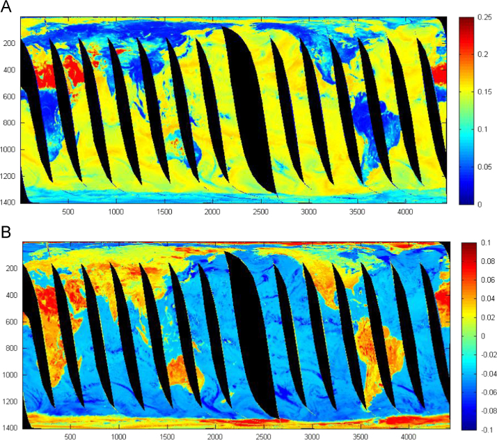
AMSR-E image with MPGR value range for (A) polarization ratio (PR 36.5) and (B) gradient ratio GR-V (36.5–18.7). In panel A, the dark red areas indicate deserts, dark blue represents dense vegetation, and the color in between correspond to mixed vegetation. In panel B, dark red highlights desert regions and light red showing vegetation condition, yellow and sky blue showing mixed vegetation (30/09/2011). Both images clearly differentiate land and water on earth after polarization or gradient ratio.
Table 3.
Land cover classes and there MPGR value.
| Land Cover Classes | PR-10 | PR-18 | PR-36 | PR-89 | GR-V (89-18) | GR-H (89-18) | GR-V (36-10) | GR-H (36-10) |
|---|---|---|---|---|---|---|---|---|
| Water | 0.20–0.25 | 0.17–0.18 | 0.035–0.04 | 0.06–0.07 | 0.10–0.11 | 0.20–0.25 | 0.10–0.11 | 0.30–0.4 |
| Evergreen Needle leaf Forest | 0.005–0.01 | 0.005–0.01 | 0.005–0.01 | 0.00–0.005 | 0.00–0.005 | 0.005–0.01 | 0.005–0.01 | 0.005–0.01 |
| Evergreen Broad leaf Forest | 0.00–0.005 | 0.00–0.005 | 0.00–0.005 | 0.00–0.005 | −0.02 to −0.03 | −0.02 to −0.03 | −0.01 to −0.005 | −0.01 to −0.005 |
| Deciduous Needle leaf Forest | 0.005–0.01 | 0.005–0.01 | 0.005–0.01 | 0.00–0.005 | 0.005–0.01 | 0.005–0.01 | 0.005–0.01 | 0.005–0.01 |
| Deciduous Broad leaf Forest | 0.005–0.01 | 0.00–0.005 | 0.00–0.005 | 0.00–0.005 | 0.00–0.005 | 0.00–0.005 | -0.005–0.0 | 0.00–0.005 |
| Mixed Forest | 0.005–0.01 | 0.00–0.005 | 0.00–0.005 | 0.00–0.005 | 0.005–0.01 | 0.005–0.01 | 0.005–0.01 | 0.005–0.01 |
| Closed Shrub lands | 0.035–0.04 | 0.025–0.03 | 0.015–0.02 | 0.01–0.015 | -0.005–0.0 | 0.015–0.02 | 0.00–0.005 | 0.02–0.025 |
| Open Shrub lands | 0.04–0.05 | 0.035–0.04 | 0.025–0.03 | 0.01–0.015 | −0.01 to −0.005 | 0.015–0.02 | -0.005–0.0 | 0.025–0.03 |
| Woody Savannas | 0.00–0.005 | 0.00–0.005 | 0.00–0.005 | 0.00–0.005 | -0.01 to −0.005 | −0.005–0.0 | −0.005–0.0 | −0.005–0.0 |
| Savannas | 0.015–0.02 | 0.01–0.015 | 0.005–0.01 | 0.00–0.005 | −0.01 to −0.005 | 0.00–0.005 | −0.005–0.0 | 0.005–0.01 |
| Grasslands | 0.04–0.05 | 0.025–0.03 | 0.015–0.02 | 0.005–0.01 | -0.005–0.0 | 0.02–0.025 | 0.005–0.01 | 0.03–0.035 |
| Permanent Wetlands | 0.035–0.04 | 0.025–0.03 | 0.02–0.025 | 0.015–0.02 | 0.02–0.025 | 0.035–0.04 | 0.015–0.02 | 0.03–0.035 |
| Croplands | 0.025–0.03 | 0.015–0.02 | 0.01–0.015 | 0.005–0.01 | 0.005–0.01 | 0.015–0.02 | 0.005–0.01 | 0.02–0.025 |
| Urban Built-up | 0.05–0.06 | 0.035–0.04 | 0.00–0.005 | 0.01–0.015 | 0.025–0.03 | 0.05–0.06 | 0.00–0.005 | 0.05–0.06 |
| Cropland Natural Vegetation Mosaic | 0.03–0.035 | 0.02–0.025 | 0.01–0.015 | 0.00–0.005 | 0.01–0.015 | 0.025–0.03 | 0.01–0.015 | 0.03–0.035 |
| Snow Ice | 0.13–0.14 | 0.11–0.12 | 0.07–0.08 | 0.05–0.06 | −0.01 to −0.005 | 0.05–0.06 | −0.02 to −0.01 | 0.05–0.06 |
| Barren Sparsely Vegetated | 0.09–0.10 | 0.07–0.08 | 0.05–0.06 | 0.035–0.04 | −0.005–0.0 | 0.04–0.05 | −0.005–0.0 | 0.04–0.05 |
Fig. 3.
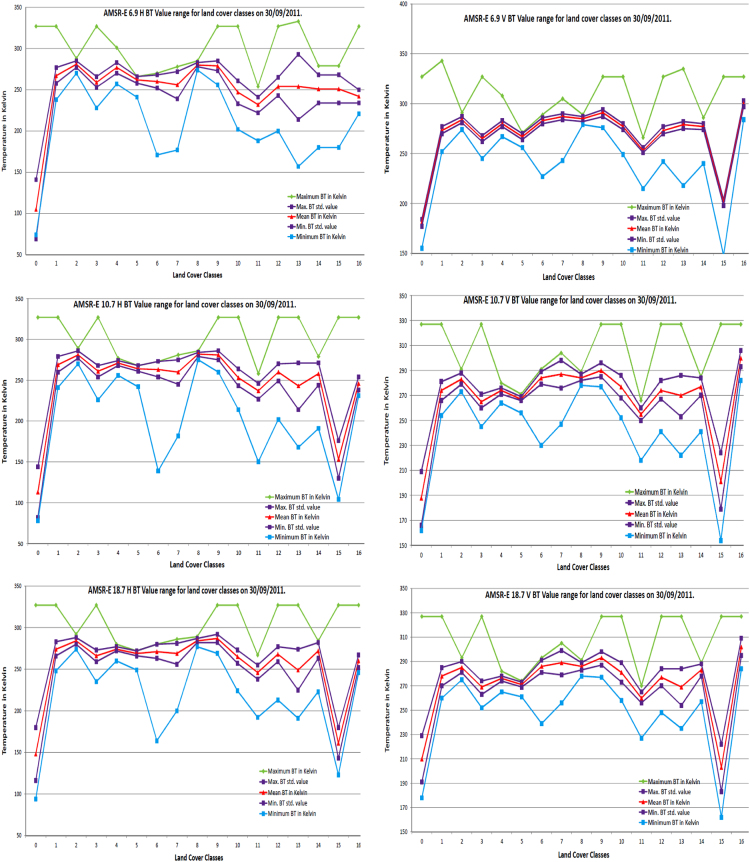
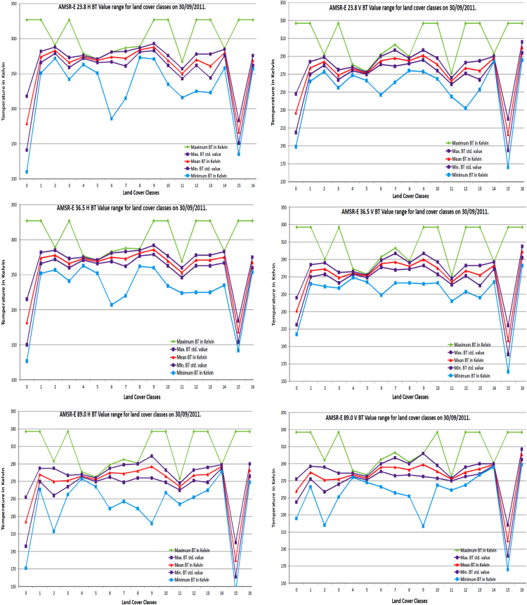
Seventeen land cover classes maximum, minimum, mean and standard deviation temperature in kelvin for 6.9, 10.7, 18.7, 23.8, 36.5 and 89.0 GHz AMSR-E frequency.
2. Experimental design, materials and methods
The experiments were carried out in Satellite Climate Studies Branch (NOAA) with the help of Goddard Space Flight Centre NASA. The Advanced Microwave Scanning Radiometer (AMSR-E) was deployed on the NASA Earth Observing System (EOS) polar-orbiting Aqua satellite platform provides global passive microwave measurements of terrestrial, oceanic and atmospheric variables for the investigation of water and energy cycles [10], [11]. The monthly level-3 AMSR-E snow water equivalent (SWE) data AE_MoSno (AMSR-E/Aqua monthly L3 Global Snow Water Equivalent EASE-Grids) in Northern Hemisphere were obtained from the NSIDC, NOAA. These data are stored in Hierarchical Data Format–Earth Observing System (HDF–EOS) format and contain SWE data and quality assurance flags mapped to 25 km Equal-Area Scalable Earth Grids (EASE-Grids). For height information Shuttle Radar Topography Mission (SRTM) data of approximately 90 m resolution were downloaded from the USGS website and used to prepare the digital elevation map (DEM). Moderate Resolution Imaging Spectroradiometer (MODIS) land cover data (MCD12Q1) was acquired from the Goddard Space Flight Centre NASA and used to determine land cover information [12], [13]. As AMSR-E satellite data was in HDF-EOS file format so first it converted into GeoTif file format with the help of HEG tool (HDF-EOS to GeoTIFF Conversion Tool, NASA) and then projected in Lambert Azimuthal equal area projection. Once data were converted into GeoTif file format, we used ArcGIS software to generate landscape and snow cover variation data.
2.1. Snow variation data
Snow cover classification was computed from 2007 to 2011 for the months of January, April, July and October. Separate analyses were done for every 500 m elevation ranges. The snow was classified into six main classes based on SWE values: very low snow, low snow, medium snow, high snow, very high snow and extreme snow and land which was covered by snow in winter but not in other seasons were classified as “No Snow” class. Actual SWE values are scaled down by a factor of 2 for storing in the HDF-EOS file, resulting in a stored data range of 0–240. In terms of snow depth each gray level need to multiply by factor 2. This data shows snow depth from 0 to 480mm. Fig. 1 shows the seasonal variations of the snow cover area (SCA) accumulated over the whole study area (Northern Hemisphere) for January, April, July and October months from 2007 to 2011.
Snow cover classification data maps were generated for all of the five years for January, April, July and October months shown in Fig. 1 and individual class area summarized in Table 1.
Table 2 shows a more detailed analysis of snow covered areas with every 500 m elevation difference during the 2007 to 2011 seasons, for which the dynamics of SCA was the most important.
2.2. Landscape data
First we selected 17 training sites for all land cover classes. Then generate their maximum, minimum, mean and standard deviation values for all horizontal and vertical AMSR-E frequencies. By this way we identify behavior of all frequencies [14]. For land cover classification we used microwave polarization and gradient ration (MPGR) combination and derive land cover data (Fig. 2).
Fig. 3 show behavior of each land cover classes for all AMSR-E data horizontal and vertical frequencies, which help to identify specify frequency for specific land cover class.
Table 3 shows all 17 land cover classes and their specific MPGR value range in a specific frequency combination.
Acknowledgements
This author would like to express special thanks to Ralph R. Ferraro for his interest and useful suggestions during the research work. Mukesh Singh Boori was supported by the National Academy of Sciences (NAS) fellowship through National Research Council (NRC), Central Government of USA; Washington DC - USA. The author wish to extend his gratitude to the Russian Scientific Foundation (RSF), Grant no. 14-31-00014 “Establishment of a Laboratory of Advanced Technology for Earth Remote Sensing”.
Footnotes
Transparency document associated with this article can be found in the online version at doi:10.1016/j.dib.2016.11.006.
Transparency document. Supplementary material
Supplementary material
.
Supplementary material
.
Supplementary material
.
References
- 1.M.S. Boori, R.R. Ferraro, Global Land Cover classification based on microwave polarization and gradient ratio (MPGR), in: I. Ivan, I. Benenson, B. Jiang, J. Horák, J. Haworth, T. Inspektor (Eds.), Proceedings of the Geo-informatics for Intelligent Transportation, Springer International Publishing Switzerland. 71: 17-37, 10.1007/978-3-319-11463-7-2
- 2.Boori M.S., Ferraro R.R. Microwave polarization and gradient ratio (MPGR) for global land surface phenology. J. Geol. Geosci. (JGG) 2013;2(2):01–10. (ISSN 2329-6755) [Google Scholar]
- 3.Boori M.S., Choudhary K., Kupriyanoy A., Kovelskiy V. Urbanization data of Samara City, Russia. Data Brief. 2016;6:885–889. doi: 10.1016/j.dib.2016.01.056. [DOI] [PMC free article] [PubMed] [Google Scholar]
- 4.Lillesand T.M., Kiefer R.W. John Wiley and Sons; New York: 1999. Remote Sensing and Image Interpretation. [Google Scholar]
- 5.J.R. Anderson, E. Hardey, J. Roach, R.E. Witmer, A land use and land cover classification system for use with remote sensor data. US geological survey professional paper, Washington, DC, 964, 1976, pp. 28
- 6.M.S. Boori, K. Choudhary, A. Kupriyanoy, V. Kovelskiy, Four decades urban growth and land use change in Samara Russia through remote sensing and GIS techniques, in: Proceedings of the SPIE: Remote Sensing and Image Formation. Vol. 9817, 2015, pp. 01–07, 10.1117/12.2227992.
- 7.Jensen J.R., Im J. Remote sensing change detection in urban environments. In: Jensen R.R., Gatrell J.D., McLean D., editors. Geo-Spatial Technologies in Urban Environments: Policy, Practice and Pixels. 2nd ed. Springer-Verlag; Heidelberg: 2007. pp. 7–30. [Google Scholar]
- 8.United Nations, World Urbanization Prospects. The 2014 Revision. New York, 2014.
- 9.Dewan A.M., Yamaguchi Y., Rahman M.Z. Dynamics of land use/cover changes and the analysis of landscape fragmentation in Dhaka Metropolitan, Bangladesh. GeoJournal. 2012;77(3):315–330. [Google Scholar]
- 10.Mao K.B., Tang H.J., Zhou Q.B., Chern Z.X., Chen Y.Q., Zhao D.Z. A study of the relationship between AMSR-E/MPI and MODIS LAI/NDVI. Remote Sens. Land Resour. 2007;1(71):27–31. [Google Scholar]
- 11.Paloscia S., Pampaloni P. Microwave polarization index for monitoring vegetation growth. IEEE Trans. Geosci. Remote Sens. 1988;26:617–621. [Google Scholar]
- 12.Kelly R., Chang A., Tsang L., Foster J. A prototype AMSR-E global snow area and snow depth algorithm. IEEE Trans. Geosci. Remote Sens. 2003;41(2):230–242. [Google Scholar]
- 13.Boori M.S., Choudhary K., Kupriyanoy A., Kovelskiy V. Satellite data for Singapore, Manila and Kuala Lumpur city growth analysis. Data Brief. 2016;7:1576–1583. doi: 10.1016/j.dib.2016.04.028. [DOI] [PMC free article] [PubMed] [Google Scholar]
- 14.Campbell J.B. Introduction to remote sensing. 3rd ed. Guilford Press; New York: 2002. [Google Scholar]
Associated Data
This section collects any data citations, data availability statements, or supplementary materials included in this article.
Supplementary Materials
Supplementary material
Supplementary material
Supplementary material


