

Abstract
We analyze experimentally determined phase diagram of γD–βB1 crystallin mixture. Proteins are described as dumbbells decorated with attractive sites to allow inter–particle interaction. We use thermodynamic perturbation theory to calculate the free energy of such mixtures and, by applying equilibrium conditions, also the compositions and concentrations of the co–existing phases. Initially we fit the Tcloud versus packing fraction η measurements for pure (x2 = 0) γD solution in 0.1 M phosphate buffer at pH = 7.0. Another piece of experimental data, used to fix the model parameters, is the isotherm x2 vs η at T = 268.5 K, at the same pH and salt content. We use the conventional Lorentz–Berthelot mixing rules to describe cross interactions. This enables us to determine (i) model parameters for pure βB1 crystallin protein and to calculate (ii) complete equilibrium surface (Tcloud – x2 – η) for the crystallin mixtures. iii) We present the results for several isotherms, including the tie–lines, as also the temperature–packing fraction curves. Good agreement with the available experimental data is obtained. An interesting result of these calculations is an evidence of coexistence of three phases. This domain appears for the region of temperatures just out of the experimental range studied so far. The input parameters, leading good description of experimental data, revealed large difference between the numbers of the attractive sites for γD and βB1 proteins. This interesting result may be related to the fact that γD has more than nine times smaller quadrupole moment than its partner in the mixture.
1 Introduction
Much of biology depends on proteins interacting with each other – pairwise or in form of oligomers – mediated by solvent and different ligands, such as salts and excipients.1,2 We need to understand how protein molecules interact with water, ions and in–between them. The self–assembly of proteins into various structures plays a crucial role in biology. A better understanding of these processes is expected to be reached by modern computer simulations, which have become indispensable for insights into physics and chemistry. Yet, the systems of several protein species in water with salts and other co–solvents, which are relevant to biology and pharmacy, are often too big to be handled well enough by current explicit–water molecular simulations. A somewhat different, less detailed–, approach, based on the ideas of condensed matter physics has been forwarded in last decades. Interactions of mixtures of oppositely charged proteins have been studied experimentally3 and theoretically4. Important previous studies relevant to our work are listed as refs. 5 and 6. Two excellent reviews of developments in this area of research have been published recently.7,8
Proteins may self–assemble to form dense liquid phase, crystals, or amorphous aggregates, and understanding of this process is important for many reasons.2,9–11 First, the self–assembly is a step in protein crystallization; good quality crystals are needed to determine protein structure through diffraction experiments. The latter pathway is the following: soluble protein aggregates initialize the coexistence of low– and high density liquid phases, differing in protein concentration. The so–called liquid–liquid phase separation is a meta–stable stage and may further lead to crystallization. For this reason, many experimental and theoretical efforts, were invested to improve understanding of the liquid–liquid phase separation. Pioneering work of George and Wilson12, and later study of Vliegenthart and Lekkerkerker13 revealed strong correlation of liquid–liquid phase boundary with the second virial coefficient and thus inter–protein interactions. Secondly, protein self–assembling in living cells plays a key role in diseases, such as Alzheimer’s, Parkinson’s, and others.1,14,15 Thirdly, a key step in developing biotech drugs16, is to formulate proteins that do not form aggregates. The challenge is to deliver formulations with high concentrations of solutes, low viscosity and maintaining the protein therapeutics properties for at least two years. Self–assembly decreases therapeutic efficacy and increases its viscosity.
As atomistic level molecular simulations are not practical for studying phase separations in such solutions, the traditional approach is to use the colloidal model of Deryaguin–Landau–Verwey–Overbeek (DLVO).17 In this approach, proteins are treated as spheres that interact via van der Waals and screened Coulomb potentials, acting between centers of molecules. The approach proved to be unsatisfactory in several respects.1 On the other hand, many aspects of protein aggregation may be pictured by the models that include anisotropic protein–protein interactions of short range.7,8,18–21 This strategy was successfully used to model a wide class of globular proteins and to analyze the liquid–liquid phase separation22,23, crystallization24,25, osmotic pressures26, distribution of aggregates27,28, percolation threshold27, and other physico–chemical properties.21
Heras and co–workers29,30 extended these ideas to binary mixtures of equally–sized spherical particles. They examined an influence of pair potential characteristics on the phase behavior under isobaric conditions. A special interest for us is the work of Roldnán–Vargas31 and coworkers. These authors treated binary mixtures of spherical particles of different sizes and with different surface patterns. The fact that the shape of protein molecules affects the phase separation, has recently been confirmed by us. A distinct shift of liquid–liquid critical density toward lower values has been obtained in case of the associating dumbbells.32 Such a behavior was before observed experimentally for the system of Y–shaped antibodies.33 For proteins in dense mixtures near the phase separation a realistic modeling of protein shape seems to be important.
In the previous studies34,35 we applied simple models with anisotropic interactions to analyze aqueous protein solutions in presence of low–molecular–mass salts. We treated proteins as hard spheres, decorated with the square–well–energy binding sites, using Wertheim’s thermodynamic perturbation theory.36 The model provided good fits to the cloud–point temperature curves of lysozyme in buffer–salt mixtures as a function of the type and concentration of salt. The necessary condition required for such modeling to be realistic is that proteins in solution during the experiment remain in their compact form.37,38 Unfortunately, many experimentalists often do not provide this information. In the next contribution32 the approach above was extended to examine the thermodynamics of fluid with “molecules” represented by two fused hard spheres, again decorated by the attractive square–well sites. Interaction between these sites was of short–range and caused association between the fused–sphere particles. The model served to estimate the effects of non–spherical geometry of proteins on solution properties.
Here we continue with applications of simple models to protein systems. Going one step further, we treat a binary mixture of proteins with molecules of each of the respective species represented as dumbbells. In the first step we need to form the molecule (dumbbell) by fusing two hard spheres and further decorate it with attractive sites on the surface. These sites allow association between the same type of molecules (self–association) as also with molecules of the other protein species present in the system. Thermodynamic properties of the model mixture are obtained via Wertheim’s thermodynamic perturbation theory.36 We utilized the McMillan–Mayer approach, where the principal variables are concentration, chemical potential of composed solvent, and temperature. We calculated the liquid–liquid phase diagram and present the results as the volume packing fraction – composition – temperature diagram. Under such conditions the osmotic pressure follows from the equation of state. When it comes to comparison with experimental data, we chose to model γD–βB1 crystallin mixture, thoroughly studied by Wang and co–workers.39 Both proteins show significant deviations from spherical shape and resemble dumbbells40 (see Fig. 1 there in, and Fig. 6 of this paper). These proteins are of special interest: an improper functioning of γD crystallin may lead to cataract in human eyes.14 For this reason crystallins were intensively studied. The investigations include stability measurements41, influence of mutation studies42,43 and other surface modifications44, and the analysis of surface residues forming inter–protein salt bridges.45 The investigations revealed that a replacement of one single of amino acid with another may modify physiological function and/or change crystallization pathway.46–49 Investigation of this subtle phenomenon is beyond the scope of this work. In this initial study we focus to the liquid–liquid phase equilibrium, and how the latter is governed by the interactions between two protein species. We use a simple “dumbbell” protein model, coupled with the thermodynamic perturbation theory of Wertheim36, to analyze the experimental data of Wang and co–workers.39
Fig. 1.
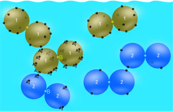
Hard spheres of equal size form dumbbells (model for protein molecule) through the sticky site B. Further interaction between protein molecules is possible through Aα sites. In this scheme m1 = 8 and m2 = 2.
Fig. 6.
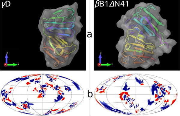
Comparison between γD (left) and βB1ΔN41 (right) crystallins. Panel a: tertiary structures embedded into solvent accessible area, generated by Schrödinger software63. Panel b: charged amino acid residues on surfaces of proteins; positive – blue, negative – red, neutral – white. The location of residues is shown in the Hammer projection64, having the polar and the azimuthal angles as the principle coordinate axes. An implementation of this projection was proposed by Koromyslova65 et al and modified by us, as described in SI.
2 Protein molecules as dumbbells decorated by attractive sites
In the first step of the calculation we compose the dumbbell–like molecules of type i with number density by dimerization of hard–spheres through the sticky sites B (see Fig. 1). The sticky BB interaction, is written as:
| (1) |
where rij denotes the distance between centers of spheres of the type i and j and Ωi,Ωj their orientations. Furthermore, zBB is the distance between sites B, denote orientation average, δ(…) is the Dirac delta function, and δij is the Kroneker delta symbol. The dumbbells are formed when and For simplicity we assume that the hard spheres forming the protein species are of equal size σ. In the experimental case analyzed here this is not far from being true. The number of the attractive sites of type Aα, located on a sphere belonging to the molecule i is mi. Further, α runs over 1,…,mi, while index i is assuming values 1 and 2. The number density of the system is .
Protein molecules i and j are interacting via the pair potential, which consists of the sum of four terms uij(rij,Ωi,Ωj). Note again that hard–spheres labeled 1 form molecules 1, while the hard–spheres denoted 2 form molecules of type 2. These terms describe the interaction between decorated hard spheres i and j, belonging to molecules i and j:
| (2) |
Here uhs(rij) is the hard–sphere potential, zαβ is the distance between sites Aα and Aβ, which belong to the spheres of the type i and j,
| (3) |
εij and ωij are the square–well depth and width, respectively. In summary, we have four types of, i.e. 1–1, 1–2, 2–1, and 2–2 interaction between the decorated hard spheres denoted 1 and 2.
3 Thermodynamic perturbation theory
Numerical results for the model described above are obtained by Wertheim’s thermodynamic perturbation theory (TPT).36 The basic quantity, Helmholtz free energy A, is composed of the ideal (id), hard–sphere (hs), and association term (ass):
| (4) |
These terms are written as:
| (5) |
| (6) |
| (7) |
where β = 1/kBT and T is the absolute temperature, Λi is the de-Broglie thermal wavelength50, ρt = ρ1 + ρ2, η = πρtσ3/6, is the Percus–Yevick expression for the contact value of the hard–sphere radial distribution function51, and Xi is the fraction of the particles not bonded at any site Aα of the hard sphere of type i. In addition we assume two types of steric incompatibilities: (i) the site Aα on one molecule cannot bond simultaneously to two Aα sites on another molecule; and (ii) double bonding between molecules is not allowed; see also Fig. 1 and the ref. 52 (Fig. 2 there in). Xi follows from the statistical–mechanical analogue of the mass action law53:
| (8) |
where
| (9) |
Here is the orientational average of the Mayer function for the square–well site–site interaction:
| (10) |
Wertheim’s TPT uses the orientation average of fij(r) and accordingly placement of the sites does not enter the theory. There is computer evidence in literature that this is not a severe approximation.54
Fig. 2.
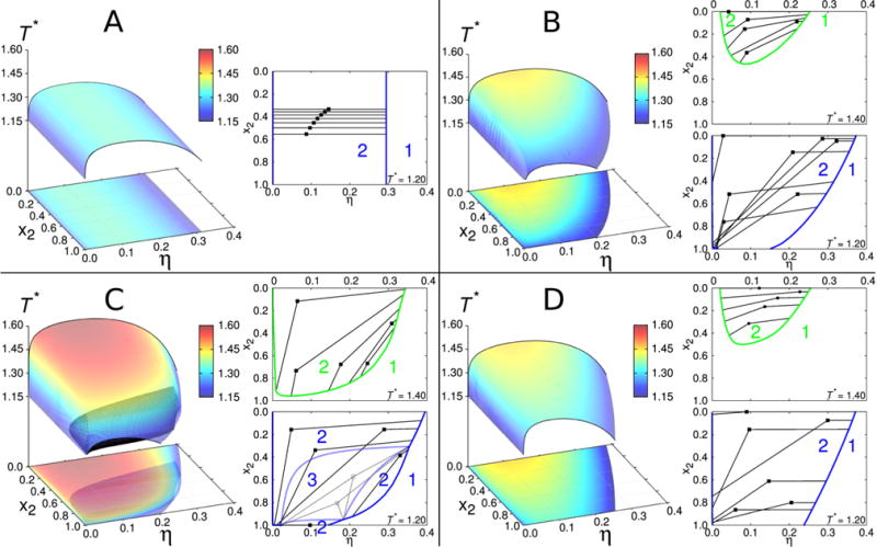
Phase diagrams for binary protein mixtures. Within each panel we present complete equilibrium surface and its projections onto η–x2 plane, as well as isotherms showing how the unstable points (denoted by filled squares) decompose into the coexisting liquid phases. Parameters for each panel read: ε11 = ε22 = 13.7ε, m1 = m2 = 4 (panel A); ε11 = ε22 = 13.7ε, m1 = 5, m2 = 3 (panel B); ε11 = 1.1ε22, ε22 = 13.7ε, m1 = 5, m2 = 3 (panel C); and ε22 = 1.1ε11, ε11 = 13.7ε, m1 = 5, m2 = 3 (panel D). The equality, ω11 = ω22 = 0.061σ, holds for all panels. The constant 13.7 was (merely for the purpose of presentation) chosen arbitrary to yield the critical temperatures in these graphs to fall between 1.15 and 1.60.
Once the free energy A is known, the chemical potential of the protein species i, and the equation of state (pressure P) can be obtained from the standard thermodynamic relations50
| (11) |
| (12) |
4 Conditions of phase equilibrium
Binary system with protein densities may undergo phase decomposition into Q phases, denoted here as (1), (2) … (γ) … (Q). According to the Gibbs phase rule Q ≤ 4. The notation denotes the (unstable) “mother” phase, while the notation applies to the (stable) “daughter” phases (γ). Thermodynamic conditions to be satisfied in equilibrium read:
| (13) |
| (14) |
In words: chemical potential of species i = 1,2 within phase (γ), must be at given temperature and pressure equal in all phases. In addition to these conditions, we need also to consider the conservation of the volume fractions of phases X(γ) = V(γ)/V(0) and the number densities of proteins over the coexisting phases (γ):
| (15) |
| (16) |
Eqs. (13–16) form the set of expressions for unknowns , X(γ) (γ = 1…Q) at specified densities of the mother phase.
In order to determine the coexistence region we need to numerically solve the set of equations defined above. This task may be accompanied by several problems. First, the solution of the system of nonlinear equations is not unique and the exact number of solutions is not known in advance. Second, numerical methods for solving nonlinear equations are usually based on iterative algorithms, requiring good initial approximation to reach the convergence. Third, in a process of searching for the solution one can get stranded at a saddle point, away from the global free energy minimum. In general, additional restrictions55 must be considered, what makes such an approach time consuming.
To avoid these complications, we used a somewhat different approach, searching for the global minimum directly. The appropriate functional to be minimized is the free energy of the system per volume, A(0)/V(0),
| (17) |
To account for the conservation conditions given by Eqs. (15) and (16), we insert these expressions into Eq. (17), and thus reduce the dimensionality of the problem. Next we use the Boltzmann simplex simulated annealing method (BSSA), described in Chapters 10.4 and 10.9 of ref. 56, to find the global minimum. When this minimum is reached, the conditions given by Eqs. (13–14), are automatically fulfilled. Numerically, the equations are satisfied within 10−2 %. More detailed description of the search for the global minimum is given as a part of the Supporting Information.
5 Binary mixture of model proteins
Our goal here is to study stability of mixtures of two protein species. The main parameters of the model are: (i) number of binding sites m1 and m2 per sphere (for protein species 1 and 2); (ii) the attractive square well depths ε11, ε22; and (iii) the corresponding interaction ranges ω11, ω22. For the cross interactions we use standard Lorentz–Berthelot mixing rules: (ε12)2 = ε11ε22 and 2ω12 = ω11 +ω22. Initially we perform a systematic analysis of how main model parameters affect the phase diagrams, presented as volume packing fraction (η) – composition – temperature (T) graphs.
Model parameters shape the phase diagram
The initial case to be examined is a mixture where both proteins have four sites per sphere, m1 = m2 = 4, equal square well depths ε11 = ε22 = 13.7ε, and corresponding ranges ω11 = ω22 = 0.061σ. In other words, we are mixing the same type of molecules. Note that in this chapter (and here only), we use the reduced units: energy is measured in ε, temperature as T∗ = kBT/ε, and length in diameter of sphere σ. Results for such a “symmetric” mixture are shown on panel A of Fig. 2. The states for temperatures below the equilibrium surface are unstable and decompose into low– and high– (volume) packing fraction (η) liquid phases. The “mixture” studied above represents the simplest possible example; it translates the symmetry of the pair potentials into topology of the phase diagram. The fact that two protein species have equal interaction parameters and sizes causes for the curves belonging different x2 values to be parallel to each other. When the phase separation occurs, the decomposition into low– and high–packing fractions is purely density driven. This is shown on the right site of panel A (two– and one–phase regions are labeled by numbers “2” and “1”, respectively). In other words, the lines connecting coexisting phases, the so–called tie lines are in this case parallel to the η axis.
To study the deviations from the basic case examined above, we place unequal numbers of sites on each protein (m1 ≠ m2), while keeping other parameters unchanged. We examine the case where m1 is increased by one (m1 = 5), and m2 decreased by one (m2 = 3). The corresponding phase diagram is shown on panel B of Fig. 2. In contrast to the previous example, the x2 curves are not parallel to each other and a distinct asymmetry along x2 axis is observed. Envelopes for pure components, denoted by black solid lines at x2 = 0 and x2 = 1, are different: protein 1 has higher critical density and temperature, since it has five attractive sites (per sphere) than the protein species labeled 2. This observation is consistent with our previous study34, as well as, with observations of other authors studying one–component systems.57,58 In addition to this, the unstable states exhibit higher complexity: as inferred from the right site of panel B, T∗ = 1.20, the high–packing fraction phase tends to retain the composition of the unstable state (density driven), while the low–packing fraction phase is enriched on an account of the second component (composition driven), to satisfy the conservation of particles. At higher temperature, T∗ = 1.40, this effect is less pronounced.
In the next example the differences between protein species are introduced on account of modifying their interaction energies εij. It is important to stress out that overall protein–protein interaction is controlled by εij and ωij, as well as, by the number of binding sites mi. Here the square well depth ε11 is increased for 10 %, while keeping the number of sites m1 = 5 and m2 = 3, and ranges ωij unchanged. These results are shown on panel C of Fig. 2. On the first sight there seems to be little difference to panel B, except for higher critical point of the envelope at x2 = 0. A closer look, however, reveals the coexistence region of three liquid phases (black shaded area), embedded into the two–phase region. Interestingly, the three–phase region disappears for the temperature equal to the critical value of pure protein 2 (x2 = 1) that is at T∗ = 1.225. To demonstrate a simultaneous presence of two– and three–phase regions, we on the same panel show also the isotherms for temperatures below and above T∗ = 1.225. The isotherm for T∗ = 1.20 reflects the presence of three–phase region, labeled by number “3”, and surrounded by closed dashed–blue loop. Unstable states within this region (denoted by empty squares) decompose into the phases with packing fraction and composition as indicated on the figure. We may call these three phases as low–, intermediate–, and high–packing fraction liquid phases. According to the Gibbs phase rule, in a two–component mixture the region where three phases are in equilibrium has only one degree of freedom, in our case this is temperature. The three–phase region separates two–phase region into three sub–regions as specified on the figure. At higher temperature, T∗ = 1.40, a simpler phase diagram having only two phases in equilibrium is re–discovered.
Finally, in contrast with the previous example, we keep ε11 =13.7ε (ε = kBT/T∗) unchanged and increase the ε22 for 10 %. As before m1 = 5 and m2 = 3. In this way we suppress – in comparison with the previous case – the interaction potential difference between the two protein species. The resulting phase diagram is shown on panel D of Fig. 2. In this case the phase behavior exhibits higher symmetry along x2 axis than in panels B and C: the shape of the envelope at x2 = 1.0 resemble the one at x2 = 0.0. Interestingly, the three–phase region shown in panel C disappears under such conditions. Because of similarity in interactions among the two protein species, the system does not need a third phase for stabilization. Furthermore, the high packing fraction (daughter) phases, derived from unstable states (mother phases), tend to retain the composition of the mother phases, similarly as before shown on panel B.
6 Analysis of experimental data for γD–βB1 mixtures
Encouraged by these results we turned to analyze experimental data for γD–βB1 protein mixtures, published in ref. 39. The authors measured the cloud point temperatures, Tcloud, as a function of composition of the mixture. The crystalline proteins γD and βB1 are approximately of the same size, what makes our analysis somewhat simpler. Experimental data are converted from the volume packing fraction values ϕ39 to corresponding η units via the relation: η = πϕNAσ3/ [3Ω(M1 + x2(M2 − M1))], where NA is Avogadro number, M1 = 20,607 g mol−1 and M2 = 27,892 g mol−1 molar masses of proteins, and Ω = 7.1·10−4 L g−1 the specific volume of proteins.39
The best–fit parameters, collected in Table 1, were determined by hand; initially we pick m1, ε11, and ω11 to fit the envelope of pure γD protein (x2 = 0.0). Experimental results for pure βB1 (x2 = 1.0) are not available and to adjust m2, ε22, and ω22 values, we fit the isotherm x2 vs η at T = 268.5 K (see Fig. 3). In this range of x2 values the Tcloud data are readily available.39 This is all the input information we use. We also assume that conventional Lorentz–Berthelot mixing rules provide a reasonable measure of the cross interactions; it is known that an excessive deviations in parameters may cause an un–physical instability of protein mixtures.59
Table 1.
Model parameters used to analyze experimental data of Wang39 et al. In agreement with crystallographic data we use σ = 2.95 nm.
| γD | βB1 | ||
|---|---|---|---|
| m1 | 8 | m2 | 2 |
| ε11/kB [K] | 2231 | ε22/kB [K] | 3248 |
| ω11 [nm] | 0.18 | ω22 [nm] | 0.21 |
Fig. 3.
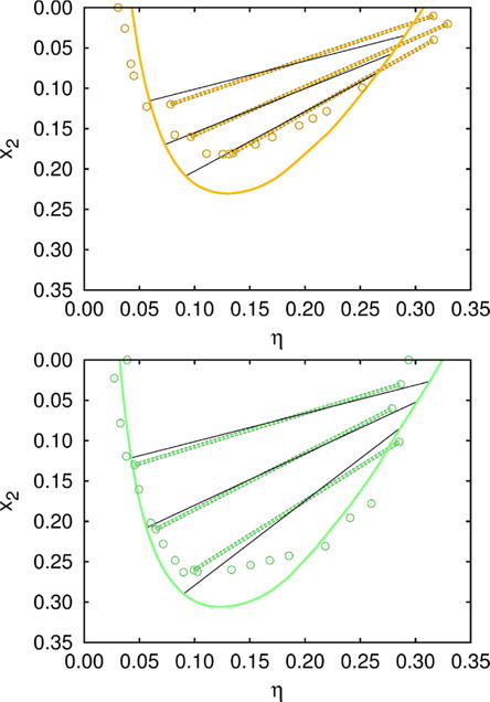
Isotherms at 268.5 K (green–bottom), and 270.5 K (orange–top). Circles show experimental data, while the solid lines represent calculations. In addition, we compare the experimentally determined tie–lines39 (dashed green/orange lines), with those calculated (black solid lines). Experimental data for the isotherm at 268.5 K (without the tie–lines) were together with the measurements for x2 = 0 (Fig. 4) used to fix the model parameters, collected in Table 1. Other results, including the isotherm at 270.5 K and the tie–lines for both temperatures, were than calculated using these values.
Parameters listed in Table 1 are then used to calculate (i) the isotherm at T = 270.5 K (including the tie–lines), for which the Tcloud measurements are available (see Fig. 3), (ii) Tcloud vs η curves for x2 equal to 0.08, 0.16, and 0.29, shown in Fig. 4 as colored curves, (iii) the isotherms at 255 K, 265 K, and 275 K presented in Fig. 5, as also (iv) the equilibrium surface for the model γD–βB1 mixture (see Fig. 4) for a range of temperatures, x2, and η values.
Fig. 4.
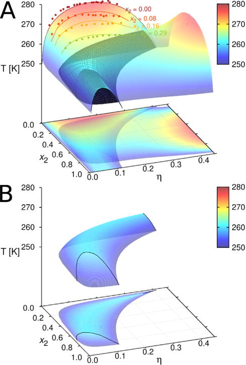
Panel A: phase separation of the γD–βB1 mixture in 0.1 M phosphate buffer at pH = 7.0. We show the equilibrium surface and its projections on the η–x2 plane. Experimental results are denoted by points and calculations by lines. The comparison is shown for x2 values equal to 0, 0.08, 0.16, and 0.29. The three–phase region (black shaded area) is embedded into two–phase region for temperatures below 264 K. Panel B: for easier visualization we re–plotted the three–phase region. Coexisting phases are denoted by black lines, see also the isotherm at T = 255 K in Fig. 5.
Fig. 5.
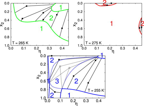
Isotherms for the temperatures 255 K, 265 K, and 275 K, extracted from Fig. 4. The color notation corresponds to the temperature code in Fig 4. The one–, two–, and three–phase regions are denoted by the appropriate numbers. Squares denote mixtures, which phase separate while the lines are connecting the mother phases with the coexisting (daughter) phases.
Results for the calculated tie–lines and isotherm at 268.5 K are, as shown in Fig. 3, in fair agreement with measurements. The fact that we obtained correct slopes for the tie–lines supports the proposed model; it is known that the latter are very sensitive on the protein–protein interactions. As concluded by Dorsaz6 et al; the difference in cross interactions for less then kBT may already invert the slope of the tie–line. Notice that uncertainties in measurements of the packing fraction and composition of the coexisting phases can be up to ±0.02.39
In Fig. 4 we show the agreement between the Tcloud measurements and theoretical calculations (lines) for x2 values equal to 0.00, 0.08, 0.16, and 0.29. In addition to these results we also show the equilibrium surface, which signals the onset of cloudiness and the coexistence of low– and high–packing fraction (η) liquid phases. Large difference between m1 (equal to eight), and m2 (equal to two) for γD and βB1, we picture this situation in Fig. 1, is needed for the model to correctly describe experimental results. This set of the mi values leads to the presence of three–phase region (black shaded area) at temperatures below 264 K, where no experimental results are available. Notice that the two–phase coexistence region is present even for packing fractions as high as η > 0.4, what was not the case when the difference between m1 and m2 was smaller (compare Fig. 2). βB1 protein exhibits a slightly longer range ω22 as also a somewhat stronger association energy ε22. The measurements of the association enthalpies60, based on the thermodynamic analysis of protein oligomerization, reveal much larger association enthalpy in case of βB1 crystallin. This finding is consistent with our calculations. It is worth mentioning that the potential parameters (ε11, ε22 and ω11, ω22) applied in this calculation fall in a broad range of hydrogen bond magnitudes61. This result is consistent with our previous findings.34
Fig. 5 presents the results for the three isotherms, which are part of the full phase–diagram shown in Fig. 4. We show the η–x2 projections of the equilibrium surface for three different temperatures: 255 K, 265 K, and 275 K. The graphs show an evolution of the phase coexistence curves with temperature. For the highest one, T = 275 K, the one–phase region is dominant; the two–phase regions only exist around x2=0 (η between 0.1 and 0.25) as also for high η values with the composition x2 between roughly 0.4 and 0.8. For somewhat lower temperature, T = 265 K, the two–phase region is much broader. The lines indicate how the unstable points (squares) phase separate into the phases having different x2, η values. For the lowest isotherm, T = 255 K, the graph is quite complex. Here we have a domain, denoted by “3”, where three liquid phases coexist. In addition both one– and two–phase regions are present. The complexity is very likely due to fact that interprotein interactions gain on their importance if temperature is lowered. See also the discussion of results presented on panel C of Fig. 4.
Although the choice of the set of parameters is not unique, there seems to be a limited number of such sets providing reasonable results. In several examples we tested the sensitivity of the parameters listed in Table 1. In one of such cases we assumed for the number of sites to be equal m1 = m2 = 8, and ranges ω11 = ω22 = 0.18 nm, while at the same time, we increased the difference between ε11 and ε22 for 12 %. With these modifications, we have not been able to reproduce the experimental isotherm at T = 268.5 K, shown in Fig. 3: the result for x2 ≈ 0.3 at η ≈ 0.14 was in our best fitting attempt too large by a factor of two. In yet another example we choose m1 = 8 (“fixed” by fitting the experiment at x2 = 0) and m2 = 4, keeping the same temperature and ω11 and ω22 values as above. Again, even upon considerable adjustment of ε22 (we took for 15 % more negative value) the agreement with experimental x2 vs η curve was poor, much poorer than in Fig. 3.
Authors of the experimental work provided data in the domain η × x2 ∈ [0,0.3] × [0,0.3]; the state points out of this range were not accessible to measurements due to the tendency of the system to solidify. We calculated the system properties for η and x2 values out of this range – no convergence problems were encountered. An example is the liquid–liquid envelope at x2 = 1, i.e. for pure βB1 protein. Unfortunately, this curve could not be obtained by direct measurements, because of the low critical temperature below −10°C.60 Addition of polyethylene glycol to the protein buffer mixture increases the critical point and allows to measure the cloud point temperatures in a wide range of protein concentrations. Such an indirect measurements60, in conjunction with extrapolation to zero concentration of polyethylene glycol, suggest for the critical point to be around 250 K. Our theoretical model yields for x2 = 1 (see Fig. 4) the value equal to 255 K. Notice again that this prediction is based on fitting the results for x2 = 0 (absence of βB1 protein) and the isotherm for the mixture at T = 268.5 K.
An alternative (and to a certain degree complementary) presentation of the information given by phase diagram in Fig. 4 and isotherms in Fig. 5 is provided by the cloud and shadow curves.62 These curves are fundamental for studying mixtures, because they show the partitioning of protein species into low– and high–packing fraction phases. These results are shown in SI as Fig. (S1).
Relating model parameters to structural information
Crystallographic data for both proteins are available from the Protein Data Bank (PDB) server. While for γD (1hk0) complete structure is provided, for βB1 only a truncated structure is available. The truncation applies to the hydrophobic tail (41 amino acids) at the N–terminus, named βB1ΔN41 (1oki). Even though the absence of hydrophobic tail may modify phase behavior60, the quasi–elastic light scattering and circular dichroism measurements of the wild–type βB1 and mutant βB1ΔN41 revealed no significant differences.60
The surface distributions of charges and insights into tertiary structures of γD and βB1ΔN41 proteins are shown in Fig. 6. Since all the measurements were performed slightly below isoelectric points of proteins (7.1), at pH equal to 7.0, the net charge of proteins is around zero (blue and red surface areas are roughly of the same size). From the Fig. 6 it is difficult to draw any firm conclusions about why the numbers of sites per sphere (m1,m2), needed to adequately describe crystalline mixture, differ from one protein to another so much. In search for some clues we turned to the Protein Dipole Moments Server66 (http://dipole.weizmann.ac.il/) for information about higher multipole terms for 1hk0 and 1oki. The results are summarized in Table 2. The two proteins are having dipole moments of similar magnitude, while βB1ΔN41 has more than nine times larger quadrupole moment than γD. This enhances the deviation from isotropic behavior and low number of sites per sphere (m2 = 2) is needed to describe highly directional interactions among βB1 proteins. There is an experimental evidence showing that β crystallin proteins form dimers and low–branched oligomers.60,67
Table 2.
Monopole (charge), dipole, and quadrupole moments for γD and βB1ΔN41 crystallins from Protein Dipole Moments Server, atomic units, see ref. 66.
| γD crystallin | ||
|---|---|---|
| charge | dipole | quadrupole |
| 0 | 191 | 110 |
|
| ||
| βB1ΔN41 crystallin (chain A) | ||
|
| ||
| charge | dipole | quadrupole |
| 0 | 260 | 1037 |
7 Conclusions
We use a simple model to calculate the phase diagram for the mixture of two proteins. Both protein species are modeled as dumbbells (two fussed hard spheres) decorated by different numbers of attractive square–well sites allowing inter–protein attraction. Major parameters of the model are: number of attractive sites per sphere forming the protein (mi; i=1,2), their attractive range and square–well depth. In the fist part of the study we investigated how the principal model parameters shape the phase diagram. This initial calculations showed that number of the attractive sites per sphere of protein plays an important role. In the second part of the study we turned to analyze the behavior of the lens proteins. The mixture of γD and βB1 crystallins was thoroughly studied experimentally by Wang39 et al, and the authors provided the cloud point temperatures for various experimental conditions. To fix the principal parameters of our model – in particular m1 and m2 and the attractive square–well depths – we fitted experimental results for pure γD protein and the isotherm for the mixture at T = 268.5 K. The cross interaction between proteins was described by the usual Lorentz–Berthelot rule. Numerical evaluation of this model was performed by Wertheim’s thermodynamic perturbation theory, which allows calculation of the measurable properties, including the complete phase diagram.
The comparison of the model calculations with experimental data for binary mixture of γD and βB1 crystallins yields the following conclusions: (i) for good agreement between theory and experiment a large difference in number of sites per sphere of protein (m1 = 8 and m2 = 2) is needed. The results are consistent with experimental findings indicating that β crystallins form small clusters with only few proteins involved. We trace this result to the large difference in the quadrupole moments between the two proteins. (ii) Our model predicts correct slopes for the tie–lines in x2 vs η graphs. (iii) The calculation yields good agreement with experimentally determined temperature–packing fraction curves for mixtures. (iv) Model provides the results for pure protein βB1, for which no direct measurements are available, and accordingly no these data were included into fitting procedure. Calculation for the critical temperature is in good agreement with the value suggested from the extrapolation of experimental data for βB1 protein. (v) The “dumbbell” model predicts a region where three liquid phase are in equilibrium – the region is just out of the domain where measurements are currently available. The calculation demonstrates, in agreement with articles listed in the recent review papers7,8, that methods of the condensed matter physics may be useful in analysis of experimental data of protein systems.
Supplementary Material
Acknowledgments
This study was supported by the Slovenian Research Agency fund (ARRS) through the Program 0103–0201, by NIH research grant (GM063592), and Young Researchers Program (M. K.) of the Republic of Slovenia.
Footnotes
Electronic Supplementary Information (ESI) available: [details of any supplementary information available should be included here]. See DOI: 10.1039/b000000x/
References
- 1.Gunton JD, Shiryayev A, Pagan DL, editors. Protein Condensation: Kinetic Pathways to Crystallization and Disease. Cambridge University Press; 2007. [Google Scholar]
- 2.Ahnert SE, Marsh JA, Hernández H, Robinson CV, Teichmann SA. Science. 2015;350:2245. doi: 10.1126/science.aaa2245. [DOI] [PubMed] [Google Scholar]
- 3.Tavares GM, Groguennes T, Hamon P, Carvalho AF, Bouhallab S. Food Hydrocoll. 2015;48:238–247. [Google Scholar]
- 4.Kurut A, Persson BA, Åkersson T, Forsman J, Lund M. J Phys Chem Lett. 2012;3:731–734. doi: 10.1021/jz201680m. [DOI] [PubMed] [Google Scholar]
- 5.Dorsaz N, Thurston GM, Stradner A, Schurtenberger P, Foffi G. J Phys Chem B. 2009;113:1693–1709. doi: 10.1021/jp807103f. [DOI] [PubMed] [Google Scholar]
- 6.Dorsaz N, Thurston GM, Stradner A, Schurtenberger P, Foffi G. Soft Matter. 2011;7:1763–1776. [Google Scholar]
- 7.Fusco D, Charbonneau P. Colloids Surf, B. 2016;137:22–31. doi: 10.1016/j.colsurfb.2015.07.023. [DOI] [PubMed] [Google Scholar]
- 8.McManus JJ, Charbonneau P, Zaccarelli E, Asherie N. Curr Op Colloid Interf Sci. 2016;22:73–79. [Google Scholar]
- 9.Fink AL. Fold Des. 1998;3:R9–R23. doi: 10.1016/S1359-0278(98)00002-9. [DOI] [PubMed] [Google Scholar]
- 10.Wang W. Int J Pharm. 2005;289:1–30. doi: 10.1016/j.ijpharm.2004.11.014. [DOI] [PubMed] [Google Scholar]
- 11.Frokjaer S, Otzen DE. Nature Reviews. 2005;4:298–306. doi: 10.1038/nrd1695. [DOI] [PubMed] [Google Scholar]
- 12.George A, Wilson WW. Acta Crystallogr D. 1994;50:361–365. doi: 10.1107/S0907444994001216. [DOI] [PubMed] [Google Scholar]
- 13.Vliegenthart GA, Lekkerkerker HNW. J Chem Phys. 2000;112:5364–5369. [Google Scholar]
- 14.Benedek GB. Invest Ophthalmol Vis Sci. 1997;38:1911–1921. [PubMed] [Google Scholar]
- 15.Ross CA, Poirier MA. Nat Med. 2004;10:S10–S17. doi: 10.1038/nm1066. [DOI] [PubMed] [Google Scholar]
- 16.Thayer AM. Chem Eng News. 2016;94:30–35. [Google Scholar]
- 17.Verwey EJW, Overbeek JTG, editors. Theory of the Stability of Lyophobic Colloids. Elsevier; 1948. [DOI] [PubMed] [Google Scholar]
- 18.Sear RP. J Chem Phys. 1999;111:4800–4806. [Google Scholar]
- 19.Anderson VJ, Lekkerkerker HNW. Nature. 2002;416:811–815. doi: 10.1038/416811a. [DOI] [PubMed] [Google Scholar]
- 20.Bianchi E, Blaak R, Likos CN. Phys Chem Chem Phys. 2011;13:6397–6410. doi: 10.1039/c0cp02296a. [DOI] [PubMed] [Google Scholar]
- 21.Lund M. Colloids Surf, B. 2016;137:17–21. doi: 10.1016/j.colsurfb.2015.05.054. [DOI] [PubMed] [Google Scholar]
- 22.Liu H, Kumar SK, Sciortino F. J Chem Phys. 2007;127:084902. doi: 10.1063/1.2768056. [DOI] [PubMed] [Google Scholar]
- 23.Gögelein C, Nägele G, Tuinier R, Gibaud T, Stradner A, Schurtenberger P. J Chem Phys. 2008;129:085102. doi: 10.1063/1.2951987. [DOI] [PubMed] [Google Scholar]
- 24.Fortini A, Sanz E, Dijkstra M. Phys Rev E. 2008;78:041402. doi: 10.1103/PhysRevE.78.041402. [DOI] [PubMed] [Google Scholar]
- 25.Fusco D, Charbonneau P. Phys Rev E. 2013;88:012721. doi: 10.1103/PhysRevE.88.012721. [DOI] [PubMed] [Google Scholar]
- 26.Moon YU, Anderson CO, Blanch HW, Prausnitz JM. Fluid Phase Equilib. 2000;168:229–239. [Google Scholar]
- 27.Tavares JM, Teixeira PIC, da Gama MMT, Sciortino F. J Chem Phys. 2010;132:234502. doi: 10.1063/1.3435346. [DOI] [PubMed] [Google Scholar]
- 28.Audus DJ, Starr FW, Douglas JF. J Chem Phys. 2016;144:074901. doi: 10.1063/1.4941454. [DOI] [PMC free article] [PubMed] [Google Scholar]
- 29.de las Heras D, Tavares JM, da Gama MMT. J Chem Phys. 2011;134:104904. doi: 10.1063/1.3561396. [DOI] [PubMed] [Google Scholar]
- 30.de las Heras D, Tavares JM, da Gama MMT. Soft Matter. 2011;7:5615–5626. [Google Scholar]
- 31.Roldnán-Vargas S, Smallenburg F, Kob W, Sciortino F. J Chem Phys. 2013;139:244910. doi: 10.1063/1.4849115. [DOI] [PubMed] [Google Scholar]
- 32.Kastelic M, Kalyuzhnyi YV, Vlachy V. Condens Matter Phys. 2016;19:23801. [Google Scholar]
- 33.Wang Y, Lomakin A, Latypov RF, Benedek GB. Proc Natl Acad Sci USA. 2011;108:16606–16611. doi: 10.1073/pnas.1112241108. [DOI] [PMC free article] [PubMed] [Google Scholar]
- 34.Kastelic M, Kalyuzhnyi YV, Hribar-Lee B, Dill KA, Vlachy V. Proc Natl Acad Sci USA. 2015;112:6766–6770. doi: 10.1073/pnas.1507303112. [DOI] [PMC free article] [PubMed] [Google Scholar]
- 35.Janc T, Kastelic M, Bončina M, Vlachy V. Condens Matter Phys. 2015;19:23601. [Google Scholar]
- 36.Wertheim MS. J Stat Phys. 1986;42:477–492. [Google Scholar]
- 37.Sarangapani PS, Hudson SD, Jones RL, Douglas JF, Pathak JA. Biophys J. 2015;108:1–14. doi: 10.1016/j.bpj.2014.11.3483. [DOI] [PMC free article] [PubMed] [Google Scholar]
- 38.Prausnitz JM. Biophys J. 2015;108:1–2. [Google Scholar]
- 39.Wang Y, Lomakin A, McManus JJ, Ogun O, Benedek GB. Proc Natl Acad Sci USA. 2010;107:13282–13287. doi: 10.1073/pnas.1008353107. [DOI] [PMC free article] [PubMed] [Google Scholar]
- 40.Serebryany E, King JA. Prog Biophys Mol Biol. 2014;115:32–41. doi: 10.1016/j.pbiomolbio.2014.05.002. [DOI] [PMC free article] [PubMed] [Google Scholar]
- 41.Broide ML, Berland CR, Pande J, Ogun OO, Benedek GB. Proc Natl Acad Sci USA. 1991;88:5660–5664. doi: 10.1073/pnas.88.13.5660. [DOI] [PMC free article] [PubMed] [Google Scholar]
- 42.Banerjee PR, Pande A, Patrosz J, Thurston GM, Pande J. Proc Natl Acad Sci USA. 2011;108:574–579. doi: 10.1073/pnas.1014653107. [DOI] [PMC free article] [PubMed] [Google Scholar]
- 43.James S, Quinn MK, McManus JJ. Phys Chem Chem Phys. 2015;17:5413. doi: 10.1039/c4cp05892e. [DOI] [PubMed] [Google Scholar]
- 44.Quinn MK, Gnan N, James S, Ninarello A, Sciortino F, Zaccarelli E, McManus JJ. Phys Chem Chem Phys. 2015;17:31177. doi: 10.1039/c5cp04463d. [DOI] [PubMed] [Google Scholar]
- 45.Basak A, Bateman O, Slingsby C, Pande A, Asherie N, Ogun O, Benedek GB, Pande J. J Mol Biol. 2003;328:1137–1147. doi: 10.1016/s0022-2836(03)00375-9. [DOI] [PubMed] [Google Scholar]
- 46.Pande A, Pande J, Asherie N, Lomakin A, Ogun O, King J, Benedek GB. Proc Natl Acad Sci USA. 2001;98:6116–6120. doi: 10.1073/pnas.101124798. [DOI] [PMC free article] [PubMed] [Google Scholar]
- 47.Evans P, Wyatt K, Wistow GJ, Bateman OA, Wallace BA, Slingsby C. J Mol Biol. 2004;343:435–444. doi: 10.1016/j.jmb.2004.08.050. [DOI] [PubMed] [Google Scholar]
- 48.McManus JJ, Lomakin A, Ogun O, Pande A, Basan M, Pande J, Benedek GB. Proc Natl Acad Sci USA. 2007;104:16856–16861. doi: 10.1073/pnas.0707412104. [DOI] [PMC free article] [PubMed] [Google Scholar]
- 49.Ji F, Jung J, Gronenborn AM. Biochemistry. 2012;51:2588–2596. doi: 10.1021/bi300199d. [DOI] [PMC free article] [PubMed] [Google Scholar]
- 50.Hansen JP, McDonald IR, editors. Theory of Simple Liquids. Elsevier; 2006. [Google Scholar]
- 51.Lebowitz JL. Phys Rev. 1964;133:A895–A899. [Google Scholar]
- 52.Jackson G, Chapman WG, Gubbins KE. Mol Phys. 1988;65:1–31. [Google Scholar]
- 53.Chapman WG, Jackson G, Gubbins KE. Mol Phys. 1988;65:1057–1079. [Google Scholar]
- 54.Bianchi E, Tartaglia P, Zaccarelli E, Scortino F. Chemical Reviews. 2008;128:144504. doi: 10.1063/1.2888997. [DOI] [PubMed] [Google Scholar]
- 55.Emelianenko M, Liu ZK, Du Q. Comput Mater Sci. 2006;35:61–74. [Google Scholar]
- 56.Press WH, Teukolsky SA, Vetterling WT, Flannery BP, editors. Numerical Recipes in Fortran 77. Cambridge University Press; 1992. [Google Scholar]
- 57.Bianchi E, Largo J, Tartaglia P, Zaccarelli E, Sciortino F. Phys Rev Lett. 2006;97:168301. doi: 10.1103/PhysRevLett.97.168301. [DOI] [PubMed] [Google Scholar]
- 58.Liu H, Kumar SK, Sciortino F, Evans GT. J Chem Phys. 2009;130:044902. doi: 10.1063/1.3063096. [DOI] [PubMed] [Google Scholar]
- 59.Stradner A, Foffi G, Dorsaz N, Thurston G, Schurtenberger P. Phys Rev Lett. 2007;99:198103. doi: 10.1103/PhysRevLett.99.198103. [DOI] [PubMed] [Google Scholar]
- 60.Annunziata O, Pande A, Pande J, Ogun O, Lubsen NH, Benedek GB. Biochemistry. 2005;44:1316–1328. doi: 10.1021/bi048419f. [DOI] [PubMed] [Google Scholar]
- 61.Xu D, Tsai CJ, Nussinov R. Protein Eng. 1997;10:999–1012. doi: 10.1093/protein/10.9.999. [DOI] [PubMed] [Google Scholar]
- 62.Sollich P. J Phys: Condens Matter. 2002;14:R79–R117. [Google Scholar]
- 63.Schrödinger Release 2015-2, Maestro, version 10.2. Schrödinger, LLC; New York, NY: 2015. [Google Scholar]
- 64.Snyder JP, editor. Map Projections: A Working Manual. U.S. Geological Survey; Washington, DC: 1987. [Google Scholar]
- 65.Koromyslova AD, Chugunov AO, Efremov RG. J Chem Inf Model. 2014;54:1189–1199. doi: 10.1021/ci500158y. [DOI] [PubMed] [Google Scholar]
- 66.Felder CE, Prilusky J, Silman I, Sussman JL. Nucleic Acids Res. 2007;35:W512–W521. doi: 10.1093/nar/gkm307. [DOI] [PMC free article] [PubMed] [Google Scholar]
- 67.Bateman OA, Lubsen NH, Slingsby C. Exp Eye Res. 2001;73:321–331. doi: 10.1006/exer.2001.1038. [DOI] [PubMed] [Google Scholar]
Associated Data
This section collects any data citations, data availability statements, or supplementary materials included in this article.