Reducing uncertainties in decadal variability of the global carbon budget with multiple datasets

Significance

The conventional approach of calculating the global carbon budget makes the land sink the most uncertain of all budget terms. This is because, rather than being constrained by observations, it is inferred as a residual in the budget equation. Here, we overcome this limitation by performing a Bayesian fusion of different available observation-based estimates of decadal carbon fluxes. This approach reduces the uncertainty in the land sink by 41% and in the ocean sink by 46%. These results are significant because they give unprecedented confidence in the role of the increasing land sink in regulating atmospheric CO₂, and shed light on the past decadal trend.

Abstract

Conventional calculations of the global carbon budget infer the land sink as a residual between emissions, atmospheric accumulation, and the ocean sink. Thus, the land sink accumulates the errors from the other flux terms and bears the largest uncertainty. Here, we present a Bayesian fusion approach that combines multiple observations in different carbon reservoirs to optimize the land (B) and ocean (O) carbon sinks, land use change emissions (L), and indirectly fossil fuel emissions (F) from 1980 to 2014. Compared with the conventional approach, Bayesian optimization decreases the uncertainties in B by 41% and in O by 46%. The L uncertainty decreases by 47%, whereas F uncertainty is marginally improved through the knowledge of natural fluxes. Both ocean and net land uptake (B + L) rates have positive trends of 29 ± 8 and 37 ± 17 Tg C⋅y⁻² since 1980, respectively. Our Bayesian fusion of multiple observations reduces uncertainties, thereby allowing us to isolate important variability in global carbon cycle processes.

The land and ocean carbon sinks provide a vital climate mitigation “service” by absorbing on average about 55% of anthropogenic CO₂ emissions from fossil fuel combustion and land use change. Research has focused on understanding the relationships between year-to-year variability in carbon sinks and climate (1, 2), as well as the long-term trend over the full instrumental period of CO₂ monitoring at the Mauna Loa station (3). Quasidecadal variations of emissions and sinks have received comparatively less attention. However, significant climate variation occurs at this specific timescale (4). Since 1980, the variable occurrence of different El Niño–Southern Oscillation events, two large volcanic eruptions (El Chichón and Pinatubo) and the recent slowdown of land surface warming have modulated the strength of carbon sinks. There are also decadal-scale changes in the rate at which human activities perturb the natural carbon cycle, in particular the recent acceleration of fossil fuel and cement emissions in the 2000s (5) and the slowdown in global land use change emissions (LUC) in the mid-2000s, which appears to be partly driven by reduced deforestation in Brazil (6).

Here, we provide a data-driven assessment of global CO₂ sources and sinks at 5-y intervals for the period of 1980–2014. We use a Bayesian fusion approach whereby different data streams of ocean and land uptake, LUC emissions, are optimally combined, and their uncertainty reduced from prior knowledge. This approach estimates the land sink constrained by data, which is a major improvement over the conventional method for calculating the global carbon budget by Ciais et al. (7) and Le Quéré et al. (8), hereafter LQ15, where the unknown land sink was determined as a residual from the other components (emissions, atmospheric increase, ocean uptake). Most of the data streams used in this analysis start in 1980, and about one-half of them give decadal mean values of natural sinks and thus do not allow us to tackle the reconstruction of interannual variability. Our choice of applying a Bayesian fusion approach to optimize 5-y average component fluxes of the global carbon budget is therefore a compromise that maximizes the use of available observations of decadal average fluxes.

The principle of the Bayesian fusion approach is to combine an a priori imperfect knowledge of fluxes with observations and their uncertainties to infer optimized estimates of fluxes. Here, we define a priori values of terms in the global carbon budget that are not from observations. Specifically, we set prior fossil fuel and cement emissions (F) from inventories and the simulated land, ocean, and land use change carbon fluxes from process-based models (Table S1). The fluxes in this study are only anthropogenic fluxes, assuming a mean CO₂ growth rate of zero during preindustrial times. Observational datasets independent from those prior values are applied to constrain land use change emissions (L), the ocean uptake of anthropogenic CO₂ (O), the land-biosphere sink (B) in ecosystems not affected by land use change, and the net land flux (B + L) (Table S2). We select the constraining data from peer-reviewed publications and evaluate their reported uncertainties and possible error correlations with each other (see details in Table S2).

Table S1.

Prior and posterior values and uncertainties (petagrams of carbon per year)

Variable	80–84	85–89	90–94	95–99	00–04	05–09	10–14
Prior
F	5.27 ± 0.28	5.79 ± 0.41	6.18 ± 0.35	6.55 ± 0.35	7.19 ± 0.39	8.40 ± 0.53	9.16 ± 0.41
O	−1.70 ± 0.50	−1.71 ± 0.50	−1.98 ± 0.50	−1.91 ± 0.50	−1.98 ± 0.50	−2.20 ± 0.50	−2.43 ± 0.50
O_adj	−1.93 ± 0.50	−1.94 ± 0.50	−2.25 ± 0.50	−2.15 ± 0.50	−2.24 ± 0.50	−2.48 ± 0.50	−2.74 ± 0.50
B	−1.31 ± 0.95	−1.89 ± 0.83	−2.06 ± 0.85	−2.08 ± 0.80	−2.31 ± 0.80	−2.43 ± 0.80	−2.37 ± 1.01
L	1.30 ± 0.62	1.39 ± 0.65	1.78 ± 0.94	1.83 ± 1.04	1.20 ± 0.70	0.94 ± 0.65	1.00 ± 0.70
Posterior
F	5.22 ± 0.27	5.77 ± 0.38	5.96 ± 0.31	6.43 ± 0.32	7.17 ± 0.33	8.03 ± 0.40	9.14 ± 0.37
O	−1.82 ± 0.40	−1.76 ± 0.33	−2.02 ± 0.19	−1.77 ± 0.22	−2.45 ± 0.24	−2.30 ± 0.24	−2.69 ± 0.26
B	−1.86 ± 0.53	−1.83 ± 0.52	−3.07 ± 0.45	−2.31 ± 0.44	−1.64 ± 0.42	−2.36 ± 0.47	−2.82 ± 0.50
L	1.43 ± 0.29	1.63 ± 0.30	1.52 ± 0.31	1.54 ± 0.29	0.96 ± 0.26	0.86 ± 0.22	1.24 ± 0.19
B + L	−0.43 ± 0.49	−0.20 ± 0.49	−1.55 ± 0.39	−0.77 ± 0.40	−0.68 ± 0.42	−1.50 ± 0.48	−1.58 ± 0.48

The adjusted O values (O_adj) from LQ15 that are not used in the optimization are also shown for a comparison with the unadjusted prior O values. The adjusted O values are, on average, 0.26 ± 0.03 Pg C⋅y⁻¹ smaller than the unadjusted ones.

Table S2.

Sources and values of different constraining data streams used in the optimization

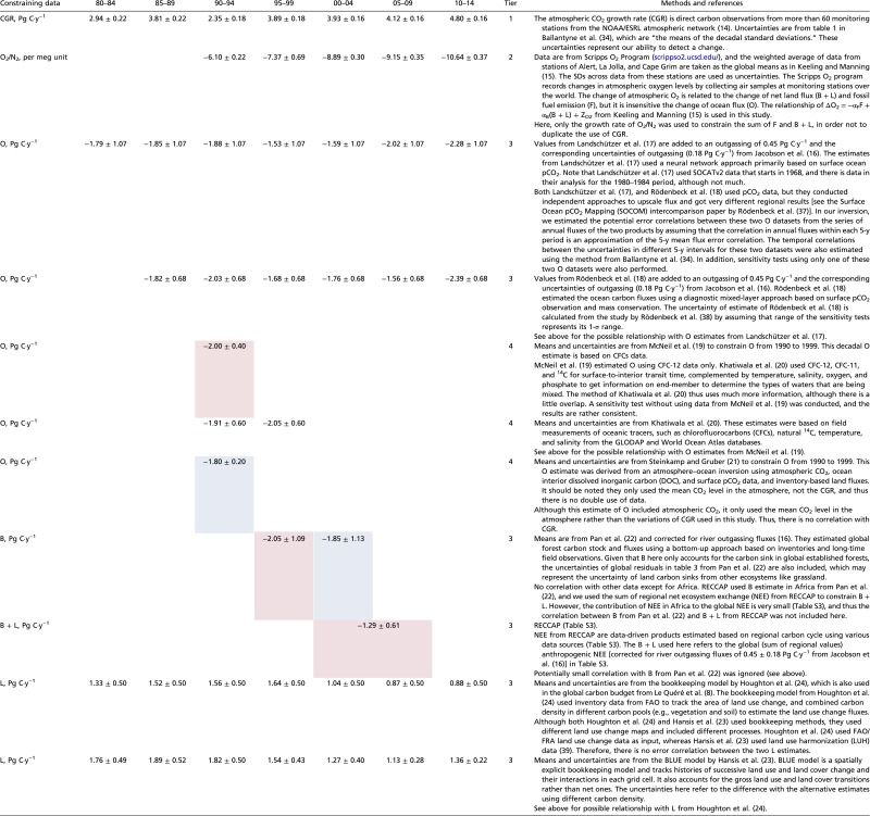The blue and orange shading indicates the length of time covered. The constraining data tiers were defined as follows: tier 1, direct carbon observations (e.g., CGR); tier 2, indirect carbon observations unambiguously related to carbon quantities (e.g., O₂/N₂); tier 3, direct carbon observations with an empirical (data-driven) model used to obtain global estimates, for example, the use of geostatistics to up-scale local data into global values; tier 4, indirect carbon observations not simply related to global carbon flux quantities.

Results

In the optimization of the global anthropogenic carbon budget (Fig. 1), the prior value of F and its uncertainty (Table S1) were defined from the mean value and the range of different fossil fuel and cement emission inventories, namely from the Carbon Dioxide Information Analysis Center (CDIAC) (9), International Energy Agency (IEA) (10), Emissions Database for Global Atmospheric Research (EDGAR) (11), and BP Statistical Review of World Energy (12). These emission inventories are not treated as direct observations of emissions, and there is currently no independent observation to verify F. The prior values of O are from seven ocean biogeochemistry models (8), and the prior values of B are from the nine TRENDY land carbon models (13). These prior values from state-of-the-art models are without direct observational constraints. Some of these models could possibly be tuned using similar observation-based data, but which observational data were used for model tuning was not explicitly reported. The prior estimates of L are derived from the difference of simulated land carbon fluxes with and without LUC in the TRENDY carbon models (13). All fluxes are defined as positive if CO₂ is emitted to the atmosphere by the land or the ocean reservoir. Uncertainties in the prior estimates of 5-yearly O, B, and L, are set to the maximum between those reported by LQ15 and the SDs across models. All uncertainties here refer to 1-σ Gaussian errors. In this context, the prior uncertainties are 0.5 for O, 0.9 for B, and 0.8 Pg C⋅y⁻¹ for L, thus not smaller than the values of 0.5, 0.8, and 0.5 Pg C⋅y⁻¹ from LQ15. It is important that the prior uncertainties are not too small, so that adding observations can adjust and constrain the sought fluxes.

Fig. 1.

The framework of our optimization. The number of constraining data streams and the specific data sources are marked on the Right. The fluxes that are optimized are 5-y averages of F, O, B, and L, representing fossil fuel and cement emissions, ocean sink, land sink, and land use change emissions, respectively. The observations used to constrain these fluxes are the 5-y averaged growth rates of CO₂ and O₂/N₂ in the atmosphere, observations of O and B from carbon measurements made in these two reservoirs, and inventory-based estimates of L and the net land sink (B + L). In this framework, the CO₂ growth rate constrains the sum of all of the fluxes. The O₂/N₂ growth rate allows us to separate O and B + L and bring some constraint on F as well.

Several independent data streams, each with their specific uncertainty and temporal averaging period (Table S2), are combined in the Bayesian optimization with the above prior knowledge. These data streams are as follows: (i) the atmospheric CO₂ growth rate (CGR) from the National Oceanic and Atmospheric Administration (NOAA)/Earth System Research Laboratory (ESRL) atmospheric network (14), which constrains the sum of all fluxes and is determined very accurately from more than 60 monitoring stations; (ii) the atmospheric 5-y mean (negative) growth rate of O₂/N₂ in the atmosphere from the Scripps O₂ Program (15), which relates to the combined effect of B + L and F changes, while being insensitive to changes in O (note that O₂/N₂ has a negative trend in the atmosphere); (iii) a set of yearly mean estimates of O from observational products based on in situ partial pressure of CO₂ (pCO₂) surveys corrected for natural ocean CO₂ outgassing from carbon delivered by rivers (16) and using a neural network approach (17) and a diagnostic mixed-layer approach (18), and a set of decadal-mean estimates of O from inventories of carbon change in the ocean deduced indirectly from chlorofluorocarbons (CFCs) (19) combined with ¹⁴C (20), and observed atmospheric mean CO₂ level and oceanic CO₂ and dissolved inorganic carbon observations (21); (iv) 10-y mean estimates of B from a global synthesis of changes in forest carbon stocks (22); (v) decadal mean B + L from inventory-based land carbon storage change from the RECCAP publications on regional budgets (Table S3); (vi) 5-y mean LUC emissions from two independent bookkeeping approaches constrained by observed carbon stocks (23, 24). The uncertainties in each data stream are either derived directly from the original publications (when reported) or estimated from expert judgments (see details in Table S2). The optimization is performed for seven consecutive 5-y windows between 1980 and 2014.

Table S3.

Estimates of net ecosystem exchange (NEE) from Regional Carbon Cycle Assessment and Processes (RECCAP) international research project

Region	Flux	Period	Mean, Tg C⋅y−1	Uncertainty, Tg C⋅y−1	References in the mass balance calculation
North America	NEE	2000–2009	−418	288	King et al. (27); Peters et al. (40)
Europe	NEE	2000–2007	−234	166	Luyssaert et al. (26); Peters et al. (40); Hartmann et al. (41)
Russia	NEE	2007–2009	−600	224	Dolman et al. (42); Hartmann et al. (41)
South Asia	NEE	2000–2009	−86	34	Liu et al. (28); Peters et al. (40); Hartmann et al. (41)
East Asia	NEE	2000–2009	−256	35	Piao et al. (25); Lauerwald et al. (43); Peters et al. (40); Hartmann et al. (41)
Southeast Asia	NEE	Undefined	−97	186	Liu et al. (28); Peters et al. (40); Hartmann et al. (41)
South America	NEE	2000–2009	11	284	Gloor et al. (44); Peters et al. (40); Hartmann et al. (41)
Africa	NEE	2000–2007	12	292	Pan et al. (22); Valentini et al. (45); Peters et al. (40); Hartmann et al. (41)
Australia	NEE	1990–2011	−71	36	Haverd et al. (46); Hartmann et al. (41)
Globe	NEE	2000–2009	−1,740	604	Sum of regional NEE
	B + L	2000–2009	−1,290	611	NEE corrected for river outgassing to ocean (16)

In brief, the observed carbon fluxes in the nine regions were evaluated and summed to give the global fluxes. NEE is calculated from the mass balance of the change in territorial carbon stocks and the lateral carbon fluxes (soil carbon export to river, river outgassing to ocean, crop and wood export) in each region. The global NEE corrected for river outgassing flux (16) is used to constrain B + L in this study. Negative values indicate a flux from the atmosphere to the land.

In the Bayesian optimization, observations that describe mean fluxes during intervals longer than 5 y are still useful to infer 5-yearly fluxes. For example, the mean ocean sink observation for the 1990s (19) constrains the two mean 5-yearly O during 1990–1999, whereas other independent observations (O₂/N₂ and CGR) help to further allocate O values between the periods 1990–1994 and 1995–1999. Despite no direct observation of F, this flux is found to be slightly improved in the Bayesian fusion, through knowledge of the other terms, and because the sum of all fluxes is very well constrained from CGR observations. We are aware that some observation-based land sink estimates have systematic errors in the way they are included in the optimization. In particular, the estimate of B from ref. 22 is only for forests and ignores other biomes. However, the Regional Carbon Cycle Assessment and Processes (RECCAP) studies (25–27) and other estimates (22, 28) of the carbon stock change in nonforest biomes suggest that the forest sink alone accounts for most of the global land sink B.

The improved global budget of anthropogenic CO₂ is shown in Fig. 2, and all data are given in Table S1. After optimization, the a posteriori uncertainty in each flux is reduced. Compared with the conventional method applied by LQ15 and IPCC-AR5 (7), uncertainties in B and O are reduced by 41% and 46% in this study. In the Bayesian data fusion, the land sink is no longer solely inferred as a residual that accumulates uncertainties from all other terms, and it exhibits a large reduction in uncertainty. The uncertainty in L decreases by 47%, but the uncertainty in F is marginally improved (by 1%) through the indirect constraints of other terms. In the absence of direct constraint on F, this small reduction in the F uncertainties compared with LQ15 and IPCC-AR5 (7) is also because we use multiple emission inventories [whereas LQ15 and IPCC-AR5 (7) only used CDIAC (9)] and start at relatively higher prior uncertainties in F (Table S1) than in LQ15. Despite their improved (smaller) uncertainties, the 5-y mean fluxes shown in Table S1 do not differ statistically in their mean values from LQ15. This indicates that each flux of the Bayesian carbon budget is fully consistent with LQ15 even though we used an array of data with different measurement methods and with uncertainties estimated in different ways. Specifically, we obtain emissions from fossil fuel burning and cement production that are smaller than LQ15 by 0.18 ± 0.19 Pg C⋅y⁻¹ during 1980–2014 (Fig. 2). A downward revision of global F is consistent with the correction of the emissions for China based on evidence of the lower carbon content for coal burned in that country (29). Compared with LQ15, the optimized ocean sink during 2000–2004 is larger by 0.22 Pg C⋅y⁻¹ but lower by 0.18 ± 0.10 Pg C⋅y⁻¹ during all of the other periods. In the past decade (2005–2014), both ocean sink and land sink from our optimization are smaller than LQ15. The optimized fluxes of L are similar to or lower than those from LQ15. The trend of F for the seven 5-y periods is positive (P = 0.003), with a probability of a positive trend for ocean and net land (B + L) uptake rates of 93%; the trend of B or L individually is not statistically significant (P = 0.23 for both). The increasing rate of ocean and net land uptake are 29 ± 8 and 37 ± 17 Tg C⋅y⁻² since 1980, respectively. Similar statistically positive trends were also found in the 5-y mean ocean and net land uptake rates between 1980 and 2014 calculated from the yearly budget updated by LQ15 (Fig. S1A). Given the robustness of O inferred by our optimization (Fig. S2), and in view of the many observations constraining this flux, there is a high confidence that the ocean sink has been increasing over time since 1980. The optimized land sink is less variable between different 5-y periods than in LQ15 (Fig. S1A). However, the ocean sink is more variable, with a SD of 0.34 Pg C⋅y⁻¹ compared with 0.27 Pg C⋅y⁻¹ by LQ15 (SDs across the seven periods analyzed).

Fig. 2.

(A) The fossil fuel and cement emissions (F), (B) ocean sink (O) and (C) net land flux (B + L), and (D) land sink (B) and land use change emissions (L) from prior knowledge, posterior results, and LQ15. All of the fluxes are 5-y means in each period. The error bars represent the 1-σ uncertainties.

Fig. S1.

(A) The temporal trend of ocean sink (O), land sink (B), land use change emissions (L), and net land flux (B + L) from our optimization and LQ15. (B) The partitioning of global total emissions (fossil fuel and cement emissions and land use change emissions, F + L) into atmosphere, ocean (O), and biosphere (B) (background shade). The markers are absolute absorbed fractions and uncertainties in ocean (blue squares) and biosphere (green squares).

Fig. S2.

Sensitivity tests using different datasets. F, O, B, L, and B + L indicate fossil fuel and cement emissions, ocean sink, land sink, land use change emissions, and net land sink, respectively. (A) Using F from different inventory datasets as priors. The bars around each flux in each period from Left to Right represent the original optimization, double prior uncertainties, prior F from IEA, prior F from EDGAR, prior F from CDIAC, and prior F from BP, respectively. (B) Using different ocean constraining datasets. The bars from Left to Right represent the original optimization (all ocean data), only data from ref. 17, only data from ref. 18, data from refs. 17 and 18 but without other ocean data, and all ocean data except ref. 19, respectively. (C) Using different tiers (tier number shown in Table S2) of constraining data. The bars from Left to Right represent the original optimization (all tiers), tier 1 only, tier 1 plus tier 2, and tier 1 plus tier 2 plus tier 3, respectively. (D) The bars from Left to Right represent the original optimization, enlarging prior uncertainties to 10⁶ Pg C⋅y⁻¹ except F, prior B, and O from CMIP5, and using a subset of constraining data including CGR, O₂/N₂, L from ref. 24 and O based on pCO₂ and inventories (17, 18, 20).

From 1980 to 2014, the average fractions of F + L emission reabsorbed by the land and ocean carbon reservoirs are 29 ± 5% (mean ± 1 σ of inter–5-y variability) and 26 ± 2%, respectively. The ratios of both O and B to F + L emission do not exhibit any significant trends (P > 0.05; Fig. S1B). Even with their reduced uncertainty in this study compared with LQ15, the variability of O and B between 5-y intervals prevents us from assessing the very small trends in their ratios to emissions. Similarly, we found no significant trend in the ratio of O or B to fossil fuel emission (F). The larger variability of the B-to-(F + L) ratios compared with the O-to-(F + L) ones (Fig. S1B) suggests that the efficiency of the land sink at absorbing emissions is more variable than that of the ocean sink. For instance, during the period that followed the cooling from the Pinatubo eruption in 1990–1994 (30–32), the B-to-(F + L) ratio increased by 46% above its long-term mean. This ratio was also higher than normal during 2005–2009, possibly due to the absence of El Niño and to the occurrence of a cooler and wetter La Niña event in 2008–2009 manifested by lower than normal CGR (3).

Discussion

In our Bayesian fusion, the CGR constrains the sum of the different fluxes; thus, an overestimation of a component flux due to the use of a single published estimate of that flux would result in an underestimation of another flux, leading to negative correlations between uncertainties in the different components of the posterior fluxes. These negative correlations are clear between uncertainties in B and F (ranging from −0.80 to −0.35), in B and O (from −0.60 to −0.30), and in B and L (from −0.53 to −0.24) (Fig. S3). This indicates that, although the uncertainties for each flux can be significantly decreased, the remaining (posterior) uncertainties are hard to be decoupled. In comparison, we also calculate the correlations between uncertainties in B and other fluxes by classical error propagation rule from mass balance equation B = CGR – F – O – L. The conventional error budget calculation gives a typical uncertainty of 0.76 Pg C⋅y⁻¹ for B. Negative error correlations also exist in that approach between B and F (−0.39), between B and O (−0.79), and between B and L (−0.39). Thus, in our study, not only the posterior uncertainties of B (0.42–0.53 Pg C⋅y⁻¹) are smaller than those calculated by the conventional approach, but also the negative error correlation between B and O is smaller, indicating a better separation between the carbon sinks of B and O. In addition, although the negative correlations between B and F, and between B and L are slightly larger than those calculated by the conventional approach, it does not mean our approach has poorer ability to separate these components because we have succeeded in significantly decreasing the absolute uncertainties for all of the fluxes, thus allowing us to draw more definitive conclusions.

Fig. S3.

Correlations between the posterior uncertainties. The subscripts 1–7 represent the 5-y periods from 1980–1984 to 2010–2014 in sequence.

The Bayesian fusion of different observational components of the anthropogenic CO₂ budget proposed in this study provides the most robust estimate to date of the strength and evolution of the land sink on 5-y intervals and brings a more robust picture of the current perturbation of the carbon cycle. Future work could apply the same fusion approach to regional carbon budget estimates and to gross CO₂ fluxes of photosynthesis, respiration, and fire emissions.

Materials and Methods

Bayesian Estimation System.

Each estimate of the 5-y mean carbon fluxes, called hereafter the “control variables” x, is based on the update from a prior estimate of these variables x^b, using some observation-based estimates y^o of the fluxes that are connected to the control variables through the relationships H: x→y = H[x]. We follow a Bayesian statistical approach for this estimation. Assuming that the distributions of uncertainties in x^b and y^o are unbiased and Gaussian, being characterized by the prior and observation uncertainty covariance matrices B and R, respectively, and that H is linear (denoted as a matrix H), the statistical estimate of x, given x^b and y^o, is unbiased and Gaussian, and the corresponding optimal estimate x^a and uncertainty covariance matrix A are given (33) as the following:

$$\mathbf{A}={\left({\mathbf{B}}^{\mathrm{-}1}+{\mathbf{H}}^{\text{T}}{\mathbf{R}}^{-1}\mathbf{H}\right)}^{-1},$$ [1]

$${\mathbf{x}}^{\text{a}}={\mathbf{x}}^{\text{b}}+\mathbf{A}{\mathbf{H}}^{\text{T}}{\mathbf{R}}^{-1}\left({\mathbf{y}}^{\text{o}}-\mathbf{H}{\mathbf{x}}^{\text{b}}\right),$$ [2]

where the superscripts T and “−1” denote the transpose and inverse of a matrix, respectively.

In the optimization, we update the estimate of the mean fluxes of fossil fuel and cement emissions (F), ocean sink (O), land sink (B), and land use change emissions (L) for each 5-y interval from 1980 to 2014 (Fig. 1 and Table S1). The observation vector contains estimates of 5-y mean global value for the following: the atmospheric growth rates of CO₂ (CGR, in petagrams of carbon per year), atmospheric growth rates of O₂/N₂ (CGR-O₂, per meg unit), observation-based estimates of ocean sinks, land sinks, land use change emissions, and net land sink (B + L) (the data sources for these components of y^o are summarized in Fig. 1 and provided in Table S2). H is defined for each 5-y interval by the following:

$$\begin{array}{l}\hspace{0.17em}\hspace{0.17em}\hspace{0.17em}\hspace{0.17em}\hspace{0.17em}\hspace{0.17em}\hspace{0.17em}\hspace{0.17em}\mathbf{x}\hspace{0.17em}\hspace{0.17em}\to \hspace{0.17em}\hspace{0.17em}\hspace{0.17em}\hspace{0.17em}\hspace{0.17em}\hspace{0.17em}\hspace{0.17em}\hspace{0.17em}\hspace{0.17em}{\mathbf{y}}^{\mathbf{o}}\hspace{0.17em}\hspace{0.17em}\hspace{0.17em}\hspace{0.17em}\hspace{0.17em}\hspace{0.17em}\hspace{0.17em}=\hspace{0.17em}\hspace{0.17em}\hspace{0.17em}\hspace{0.17em}\hspace{0.17em}\hspace{0.17em}\hspace{0.17em}\hspace{0.17em}\hspace{0.17em}\hspace{0.17em}\hspace{0.17em}\hspace{0.17em}\hspace{0.17em}\hspace{0.17em}\hspace{0.17em}\hspace{0.17em}\hspace{0.17em}\mathbf{H}\mathbf{x}\hspace{0.17em}\hspace{0.17em}\hspace{0.17em}\hspace{0.17em}\hspace{0.17em}\hspace{0.17em}\hspace{0.17em}\hspace{0.17em}\\ \mathbf{H}:\left[\begin{array}{c}\text{F}\\ \text{O}\\ \text{B}\\ \text{L}\end{array}\right]\to \left[\begin{array}{c}\text{CGR}\\ \text{CGR}-{\text{O}}_2\\ \begin{array}{c}\text{O}\\ \text{B}\end{array}\\ \begin{array}{c}\text{L}\\ \text{B}+\text{L}\end{array}\end{array}\right]=\left[\begin{array}{c}\begin{array}{c}\text{F}+\text{O}+\text{B}+\text{L}\\ {\mathrm{\alpha }}_{\text{F}}\text{F}+{\mathrm{\alpha }}_B(\text{B}+\text{L})+{\text{Z}}_{\text{O}2}\\ \text{O}\end{array}\\ \text{B}\\ \text{L}\\ \text{B}+\text{L}\end{array}\right],\end{array}$$ [3]

where α_F, α_B, and Z_O2 are constant coefficients from ref. 15.

The prior estimates for the different control variables are built with independent datasets so that there are no correlations between the prior uncertainties in the different control variables. When setting up the observation covariance matrix, the temporal correlations between the uncertainties in different 5-y intervals for CGR and O are estimated using the method in ref. 34. The correlations between the uncertainties in the two data-driven estimates of O (17, 18) are estimated from the series of annual fluxes of the two products by assuming that the correlation in annual fluxes within each 5-y period is an approximation of the 5-y mean flux error correlation.

Data Used to Derive the Prior Statistics of the Control Variables.

To define the prior estimate of F, individual country data from four emission inventories [CDIAC (9), IEA (10), EDGAR (11), and BP (12)] are grouped into geographic regions as specified by the United Nations Statistics Division (unstats.un.org/unsd/methods/m49/m49regin.htm). Cement emissions from EDGAR are added into the IEA and BP datasets that do not include cement emissions. Uncertainties for each country (35) are used to create regional uncertainty distributions using a bootstrapping method, with the uncertainties of the highest emitters in each region contributing the most to the uncertainty distributions. This effect is achieved by weighting the sampling probability (P_s) by the relative contribution of each country’s emissions (E_C) to the total emissions within the region (E_R) as follows:

$$P_s=\frac{E_C}{E_R}.$$ [4]

To constrain the temporal component of the emission errors, 10 random samples are drawn from the corresponding regional uncertainty distribution for each country, producing 10 random uncertainties for each country. These country-level uncertainties are used to constrain a random error time series covering 1980–2014, which is then run through an algorithm incorporating autocorrelated random noise, such that

$${\epsilon }_{F\left(t\right)}=0.95\times {\epsilon }_{F\left(t-1\right)}+{\epsilon }_{\left(t\right)},$$ [5]

where emission error factors for any given year ε_F(t) are correlated with the emission errors from the previous year ε_F(t−1) by an autoregressive coefficient of 0.95 with ε_(t) as random error. The autocorrelated time series are then multiplied and added to the fossil fuel emissions for each country, and subsequently 500 samples of global fossil fuel emissions are taken for each 5-y bin. The means and SDs of each bin for each inventory are calculated from these 500 samples. Additionally, the correlation in global uncertainty is calculated between 5-y bins and inventories to produce an error-covariance matrix. The maximum between the uncertainties calculated above and the SDs of the 5-y means across four emission inventories were adopted as the uncertainties in the prior estimate of F.

Prior O values are set from the ocean biogeochemistry model values used in LQ15, which represent state-of-the-art ocean models and are generally consistent with estimates from data-based products (8). Note that LQ15 adjusted their simulated O so as to match ocean observations during the decade of the 1990s and then used these bias-corrected ocean models outside this period (see adjusted values in Table S1). Here, for setting the prior O estimate and uncertainty, we consider simply the spread and the mean of ocean models without any adjustment, because the adjustment performed by LQ15 is already a kind of model data-fusion approach based on the ocean observations used in our study.

Prior values of L and B are set from simulations in the TRENDY (version 2) model intercomparison project (13). The simulations in TRENDY (version 2) are up to 2012, and thus the priors for the period of 2010–2012 were used for the period of 2010–2014. All of the prior flux values are summarized in Table S1.

Uncertainty Correlations Between Optimized Variables.

The correlations of the uncertainties between optimized variables are shown in Fig. S3. In comparison, we also calculate the correlations between uncertainties in the fluxes when deriving the estimate of B using the classical mass balance equation B = CGR – F – O – L. First, the uncertainties in an estimate of the flux i is calculated using inverse variance method, based on the variances associated with all of the estimates of this flux (j = 1, 2, …, m):

$${\sigma }_i=\sqrt{\frac{1}{{{\displaystyle \sum }}_{j=1}^m\frac{1}{{\sigma }_{i,j}^2}}}.$$ [6]

The resulting uncertainties for CGR, F, O, and L are as follows: 0.2, 0.3, 0.6, and 0.3 Pg C⋅y⁻¹, respectively. Based on a simple error propagation: ${\epsilon }_B={\epsilon }_{CGR}-{\epsilon }_F-{\epsilon }_O-{\epsilon }_L$ and the independence of the estimates of CGR, F, O, and L, the variance of the uncertainty in B is given by the following:

$${\sigma }_B^2=E\left({\epsilon }_B^T{\epsilon }_B\right)={\sigma }_{CGR}^2+{\sigma }_F^2+{\sigma }_O^2+{\sigma }_L^2,$$ [7]

where E(.) is the expectation of a variable. The correlation between the uncertainties in B and in another variable, namely, O in the equation below, is given by the following:

$$r\left({\epsilon }_B,{\epsilon }_O\right)=\frac{E\left({\epsilon }_B^T{\epsilon }_O\right)}{{\sigma }_B{\sigma }_O}=-\frac{{\sigma }_O}{{\sigma }_B}.$$ [8]

Sensitivity Tests.

Four sets of sensitivity tests were conducted (Fig. S2): (i) using F from different inventory datasets (IEA, EDGAR, CDIAC, and BP, respectively) as priors; (ii) using different ocean constraining datasets (only data from ref. 17, only data from ref. 18, data from refs. 17 and 18 but without other ocean data, and all ocean data except ref. 19, respectively); (iii) using different tiers of constraining data (tier 1 only, tier 1 plus tier 2, and tier1 plus tier 2 plus tier 3, respectively); and (iv) using enlarged prior uncertainties (10⁶ Pg C⋅y⁻¹ except F), prior B and O from CMIP5 models (36) instead of TRENDY (version 2) models, and a subset of constraining data including CGR, O₂/N₂, L from ref. 24 and O from pCO₂ and inventories (17, 18, 20). The constraining data tiers (Table S2) were defined as follows: tier 1, direct carbon observations (e.g., CGR); tier 2, indirect carbon observations unambiguously related to carbon quantities (e.g., O₂/N₂); tier 3, direct carbon observations with an empirical (data-driven) model used to obtain global estimates, for example, the use of geostatistics to up-scale local data into global values; tier 4, indirect carbon observations not simply related to global carbon flux quantities.

The ocean sink is rather consistent in all sensitivity tests (Fig. S2), implying it is very robustly constrained in the optimization because of the sufficient number and consistency of constraining observational data (see the O constraining data in Table S2). Small changes in optimized F were found (Fig. S2A) in the sensitivity tests using prior F from different datasets, and the land sink is more dependent on the prior F choice. In the sensitivity tests using different ocean constraining data (Fig. S2B), all fluxes are generally consistent, and very slight changes for O appear in the tests using ocean data from ref. 17 only and from ref. 18 only during 2000–2004 and 2005–2009. The decadal estimates (19–21) only have small impact on their corresponding periods. The important point for the sensitivity tests using different tiers of constraining data are that there is no inconsistency (i.e., shift in posterior estimate) between the assimilations of different “observation-based” tiers, although L may change due to the lack of individual constraints in tier 1 and tier 1 plus tier 2 (Fig. S2C). With enlarged prior uncertainties (10⁶ Pg C⋅y⁻¹ except F), the mean flux values do not shift in general but the posterior uncertainties increase (Fig. S2D). Results are also very consistent by replacing prior B and O from TRENDY, version 2, models with from CMIP5 models (Fig. S2D). The sensitivity test using a subset of constraining data underestimate B and L compared with the original optimized results (Fig. S2D) because the L estimates in ref. 23 (used in the original optimization but not in this sensitivity test) is higher than that in ref. 24 (Table S2).

Trend Test.

A Mann–Kendall statistical test was applied as a trend test.

References

- 1.Wang X, et al. A two-fold increase of carbon cycle sensitivity to tropical temperature variations. Nature. 2014;506(7487):212–215. doi: 10.1038/nature12915. [DOI] [PubMed] [Google Scholar]
- 2.Poulter B, et al. Contribution of semi-arid ecosystems to interannual variability of the global carbon cycle. Nature. 2014;509(7502):600–603. doi: 10.1038/nature13376. [DOI] [PubMed] [Google Scholar]
- 3.Le Quéré C, et al. Trends in the sources and sinks of carbon dioxide. Nat Geosci. 2009;2(12):831–836. [Google Scholar]
- 4.Ghil M, Vautard R. Interdecadal oscillations and the warming trend in global temperature time series. Nature. 1991;350(6316):324–327. [Google Scholar]
- 5.Raupach MR, et al. Global and regional drivers of accelerating CO2 emissions. Proc Natl Acad Sci USA. 2007;104(24):10288–10293. doi: 10.1073/pnas.0700609104. [DOI] [PMC free article] [PubMed] [Google Scholar]
- 6.Song X-P, Huang C, Saatchi SS, Hansen MC, Townshend JR. Annual carbon emissions from deforestation in the Amazon Basin between 2000 and 2010. PLoS One. 2015;10(5):e0126754. doi: 10.1371/journal.pone.0126754. [DOI] [PMC free article] [PubMed] [Google Scholar]
- 7.Ciais P, et al. Carbon and other biogeochemical cycles. In: Stocker TF, et al., editors. Climate Change 2013: The Physical Science Basis. Contribution of Working Group I to the Fifth Assessment Report of the Intergovernmental Panel on Climate Change. Cambridge Univ Press; Cambridge, UK: 2013. pp. 465–570. [Google Scholar]
- 8.Le Quéré C, et al. Global carbon budget 2014. Earth Syst Sci Data. 2015;7:47–85. [Google Scholar]
- 9.Boden TA, Marland G, Andres RJ. 2013. Global, Regional, and National Fossil-Fuel CO2Emissions (Carbon Dioxide Information Analysis Center, Oak Ridge National Laboratory Oak Ridge, TN; US Department of Energy, Oak Ridge, TN)
- 10.International Energy Agency 2013. CO2Emissions from Fuel Combustion: Highlights. IEA Statistics (International Energy Agency, Paris)
- 11.Olivier JGJ, Janssens-Maenhout G, Peters JAHW. Trends in Global CO2 Emissions: 2014 Report. PBL Netherlands Environmental Assessment Agency; The Hague: 2014. [Google Scholar]
- 12.BP . BP Statistical Review of World Energy 2015. BP; London: 2015. [Google Scholar]
- 13.Sitch S, et al. Recent trends and drivers of regional sources and sinks of carbon dioxide. Biogeosciences. 2015;12(3):653–679. [Google Scholar]
- 14. NOAA/ESRL, NOAA/ESRL calculation of global means. Available at www.esrl.noaa.gov/gmd/ccgg/about/global_means.html. Accessed August 9, 2015.
- 15.Keeling RF, Manning C. Studies of Recent Changes in Atmospheric O2 Content. 2nd Ed Elsevier; Amsterdam: 2014. [Google Scholar]
- 16.Jacobson AR, Fletcher SEM, Gruber N, Sarmiento JL, Gloor M. A joint atmosphere-ocean inversion for surface fluxes of carbon dioxide: 1. Methods and global-scale fluxes. Global Biogeochem Cycles. 2007;21(1):GB1019. [Google Scholar]
- 17.Landschützer P, Gruber N, Bakker DCE, Schuster U. Recent variability of the global ocean carbon sink. Global Biogeochem Cycles. 2014;28(9):927–949. [Google Scholar]
- 18.Rödenbeck C, et al. Interannual sea–air CO2 flux variability from an observation-driven ocean mixed-layer scheme. Biogeosciences. 2014;11(17):4599–4613. [Google Scholar]
- 19.McNeil BI, Matear RJ, Key RM, Bullister JL, Sarmiento JL. Anthropogenic CO2 uptake by the ocean based on the global chlorofluorocarbon data set. Science. 2003;299(5604):235–239. doi: 10.1126/science.1077429. [DOI] [PubMed] [Google Scholar]
- 20.Khatiwala S, Primeau F, Hall T. Reconstruction of the history of anthropogenic CO2 concentrations in the ocean. Nature. 2009;462(7271):346–349. doi: 10.1038/nature08526. [DOI] [PubMed] [Google Scholar]
- 21.Steinkamp K, Gruber N. A joint atmosphere-ocean inversion for the estimation of seasonal carbon sources and sinks. Global Biogeochem Cycles. 2013;27(3):732–745. [Google Scholar]
- 22.Pan Y, et al. A large and persistent carbon sink in the world’s forests. Science. 2011;333(6045):988–993. doi: 10.1126/science.1201609. [DOI] [PubMed] [Google Scholar]
- 23.Hansis E, Davis SJ, Pongratz J. Relevance of methodological choices for accounting of land use change carbon fluxes. Global Biogeochem Cycles. 2015;29(8):1230–1246. [Google Scholar]
- 24.Houghton RA, et al. Carbon emissions from land use and land-cover change. Biogeosciences. 2012;9(12):5125–5142. [Google Scholar]
- 25.Piao SL, et al. The carbon budget of terrestrial ecosystems in East Asia over the last two decades. Biogeosciences. 2012;9(9):3571–3586. [Google Scholar]
- 26.Luyssaert S, et al. The European land and inland water CO2, CO, CH4 and N2O balance between 2001 and 2005. Biogeosciences. 2012;9(8):3357–3380. [Google Scholar]
- 27.King AW, et al. North America’s net terrestrial CO2 exchange with the atmosphere 1990–2009. Biogeosciences. 2015;12(2):399–414. [Google Scholar]
- 28.Liu YY, et al. Recent reversal in loss of global terrestrial biomass. Nat Clim Chang. 2015;5(5):470–474. [Google Scholar]
- 29.Liu Z, et al. Reduced carbon emission estimates from fossil fuel combustion and cement production in China. Nature. 2015;524(7565):335–338. doi: 10.1038/nature14677. [DOI] [PubMed] [Google Scholar]
- 30.Lucht W, et al. Climatic control of the high-latitude vegetation greening trend and Pinatubo effect. Science. 2002;296(5573):1687–1689. doi: 10.1126/science.1071828. [DOI] [PubMed] [Google Scholar]
- 31.Mercado LM, et al. Impact of changes in diffuse radiation on the global land carbon sink. Nature. 2009;458(7241):1014–1017. doi: 10.1038/nature07949. [DOI] [PubMed] [Google Scholar]
- 32.Frölicher TL, Joos F, Raible CC, Sarmiento JL. Atmospheric CO2 response to volcanic eruptions: The role of ENSO, season, and variability. Global Biogeochem Cycles. 2013;27(1):239–251. [Google Scholar]
- 33.Tarantola A. Inverse Problem Theory and Methods for Model Parameter Estimation. SIAM; Philadelphia: 2005. [Google Scholar]
- 34.Ballantyne AP, et al. Audit of the global carbon budget: Estimate errors and their impact on uptake uncertainty. Biogeosciences. 2015;12(8):2565–2584. [Google Scholar]
- 35.Andres RJ, Boden TA, Higdon D. A new evaluation of the uncertainty associated with CDIAC estimates of fossil fuel carbon dioxide emission. Tellus B Chem Phys Meterol. 2014;66:23616. [Google Scholar]
- 36.Anav A, et al. Evaluating the land and ocean components of the global carbon cycle in the CMIP5 earth system models. J Clim. 2013;26(18):6801–6843. [Google Scholar]
- 37.Rödenbeck C, et al. Data-based estimates of the ocean carbon sink variability—first results of the surface ocean pCO2 mapping intercomparison (SOCOM) Biogeosciences. 2015;12(23):7251–7278. [Google Scholar]
- 38.Rödenbeck C, et al. Global surface-ocean pCO2 and sea–air CO2 flux variability from an observation-driven ocean mixed-layer scheme. Ocean Sci. 2013;9(2):193–216. [Google Scholar]
- 39.Hurtt GC, et al. Harmonization of land-use scenarios for the period 1500–2100: 600 years of global gridded annual land-use transitions, wood harvest, and resulting secondary lands. Clim Change. 2011;109(1-2):117–161. [Google Scholar]
- 40.Peters GP, Davis SJ, Andrew R. A synthesis of carbon in international trade. Biogeosciences. 2012;9(8):3247–3276. [Google Scholar]
- 41.Hartmann J, Jansen N, Dürr HH, Kempe S, Köhler P. Global CO2-consumption by chemical weathering: What is the contribution of highly active weathering regions? Global Planet Change. 2009;69(4):185–194. [Google Scholar]
- 42.Dolman AJ, et al. An estimate of the terrestrial carbon budget of Russia using inventory-based, eddy covariance and inversion methods. Biogeosciences. 2012;9(12):5323–5340. [Google Scholar]
- 43.Lauerwald R, Laruelle GG, Hartmann J, Ciais P, Regnier PAG. Spatial patterns in CO2 evasion from the global river network. Global Biogeochem Cycles. 2015;29(5):2014GB004941. [Google Scholar]
- 44.Gloor M, et al. The carbon balance of South America: A review of the status, decadal trends and main determinants. Biogeosciences. 2012;9(12):5407–5430. [Google Scholar]
- 45.Valentini R, et al. A full greenhouse gases budget of Africa: Synthesis, uncertainties, and vulnerabilities. Biogeosciences. 2014;11(2):381–407. [Google Scholar]
- 46.Haverd V, et al. The Australian terrestrial carbon budget. Biogeosciences. 2013;10(2):851–869. [Google Scholar]