

Abstract
Which principles determine the organization of the intricate network formed by nerve fibers that link the primate cerebral cortex? We addressed this issue for the connections of primate visual cortices by systematically analyzing how the existence or absence of connections, their density as well as laminar patterns of projection origins and terminations are correlated with distance, similarity in cortical type as well as neuronal density or laminar thickness of cortical areas. Analyses were based on four extensive compilations of qualitative as well as quantitative data for connections of the primate visual cortical system in macaque monkeys (Felleman and Van Essen, 1991; Barbas, 1986; Barbas and Rempel-Clower, 1997; Barone et al., 2000; Markov et al., 2014). Distance and thickness similarity were not consistently correlated with connection features, but similarity of cortical type, determined by qualitative features of laminar differentiation, or measured quantitatively as the areas' overall neuronal density, was a reliable predictor for the existence of connections between areas. Cortical type similarity was also consistently and closely correlated with characteristic laminar connection profiles: structurally dissimilar areas had origin and termination patterns that were biased to the upper or deep cortical layers, while similar areas showed more bilaminar origins and terminations. These results suggest that patterns of corticocortical connections of primate visual cortices are closely linked to the stratified architecture of the cerebral cortex. In particular, the regularity of laminar projection origins and terminations arises from the structural differences between cortical areas. The observed integration of projections with the intrinsic cortical architecture provides a structural basis for advanced theories of cortical organization and function.
Introduction
Macroscopic connections among cortical areas form intricate networks for neural communication (Van Essen et al., 2013). These networks are neither completely nor randomly wired, and their organization has been the subject of extensive investigations (reviewed in Sporns et al., 2004; Bullmore and Sporns, 2009; Sporns, 2010).
An essential question is what determines the existence or absence of connections, since not all possible connections exist. A starting point is the observation that neighboring areas or neighbors-one-over are frequently connected (Barbas and Pandya, 1989), accounting for about half of the connections in primate visual cortex (Young, 1992). While proximity may contribute to the formation of connections (Ercsey-Ravasz et al., 2013), it cannot be the only factor, because some connections extend across considerable distances (e.g., Barbas and Mesulam, 1981; Kaiser and Hilgetag, 2006; Markov et al., 2013). Another model suggests that connections are formed between areas of similar thickness (He et al., 2007; Bassett et al., 2008; He et al., 2008; Liu et al., 2008; Bassett and Bullmore, 2009; He et al., 2009). Alternatively, a structural model posits that similarities in overall laminar organization (Barbas, 1986; Barbas and Rempel-Clower, 1997; Medalla and Barbas, 2006) help explain the presence and patterns of connections (Barbas and Rempel-Clower, 1997; Barbas et al., 2005a).
An important feature of connections is their strength—the number of neurons in a pathway – that may help estimate functional impact (Vanduffel el al. 1997). Strength varies considerably across pathways (MacNeil et al., 1997; Scannell et al., 2000; Hilgetag et al., 2000b) and possesses a logarithmic (Scannell et al., 2000) or lognormal (Markov et al., 2011) global distribution, where a few pathways are very dense and most others are either sparse or absent. The factors that underlie this distribution are still incompletely understood (Kaiser et al., 2009).
A further question concerns the laminar patterns of connections [reviewed in Felleman and Van Essen (1991)], which emanate and terminate in functionally distinct laminar micro-environments (Barbas et al., 2005b). Laminar patterns of connections are diverse but strikingly repetitive. For example, in the cortical visual system connections can be arranged into sequences or hierarchies. In such sequences, projections that mostly originate from upper cortical layers and terminate in the middle-to-deep layers (‘feedforward’) point in one direction, while the reciprocal (‘feedback’) projections that mostly originate from deep layers and terminate in upper cortical layers point in the opposite direction of the sequence. Most visual projections fit such a scheme, with only 6 violations out of 318 patterns (Hilgetag et al., 1996). By contrast, if such arrangements are attempted for randomly assigned projection patterns, a large number of disagreements (>100) remain (Hilgetag et al., 2000c). Thus, laminar projection patterns demonstrate a remarkably regular motif in cortical organization. It has been suggested that the regularity depends on cortical structure (Barbas, 1986; Barbas and Rempel-Clower, 1997), physical distance (Bullier and Nowak, 1995), or hierarchical rank (Barone et al., 2000).
Here we systematically investigated factors that contribute to the organization of cortical connections, by quantitative hypothesis testing based on distinct proposed models. To test these models, we studied extensive data from various sources to increase the reliability and generality of the findings: a collation of qualitatively described primate visual connections (Felleman and Van Essen, 1991); quantitative datasets from the laboratory of Kennedy (Barone et al., 2000; Markov et al., 2014); and newly compiled quantitative data on connections and cortical structure from our laboratory (Barbas, 1986; Barbas and Rempel-Clower, 1997). The primate visual cortical system is ideal for this study, because extensive available data make it possible to test to what extent alternative models, based on differences in distance, cortical thickness, or cortical structure between connected areas best account for the existence, absence, density and laminar distribution of connections. Preliminary results from this study were presented in abstract form (Hilgetag et al., 2008).
Methods
Connection datasets
We analyzed the following four datasets which provide qualitative and quantitative information on the existence or absence, strength, as well as laminar patterns of projection neurons in the primate visual cortex in macaque monkeys. These data include the landmark compilation of Felleman and Van Essen of visual connections (1991), two sets of quantitative laminar projection patterns for visual projections (Barone et al., 2000; Markov et al., 2014), as well as a partly independent set of prefrontal afferent neurons originating in visual cortex. The latter data have been recompiled from published studies of our laboratory (Barbas, 1986; 1993; Barbas and Rempel-Clower, 1997) and are comprehensively presented in the present paper for the first time. Essential features of the analyzed datasets are summarized in Table 1. We used statistical approaches, such as rank correlations, that are appropriate for the respective data scales. Probabilities of the findings are reported at levels p>0.05, p<0.05, and p<0.001, and findings were considered significant if p<0.05.
Table 1. Essential features of the analyzed datasets.
| Dataset | Analyzed feature | Data scale |
|---|---|---|
| Global visual connections (Felleman and Van Essen, 1991) | Existence/absence of projections | Qualitative (Nominal) |
| Laminar projection origins and terminations | Qualitative (Ordinal) | |
| Visual prefrontal afferents (Barbas, 1986; Barbas, 1993; Barbas and Rempel-Clower, 1997; Table 2) | Existence/absence and strength of projections | Qualitative (Nominal), Quantitative (Ratio) |
| Laminar projection origins | Quantitative (Ratio) | |
| V1 and V4 afferents (Barone et al., 2000) | Laminar projection origins | Quantitative (Ratio) |
| Global visual afferents (Markov et al., 2014) | Laminar projection origins | Quantitative (Ratio) |
Dataset 1: ‘Global visual connections.’
The dataset derives from Felleman and Van Essen's compilation of qualitative information on the existence and absence as well as laminar patterns of connections among areas of the primate cortical visual system (Felleman and Van Essen, 1991). For all analyses reported here, areas MIP and MDP were excluded due to limited information about their connections. Moreover, subdivisions of areas PIT (PITd, PITV), CIT (CITd, CITv), AIT (ATId, AITv) and STP (STPp, STPa) were considered separately, and information that was available for a whole area (such as PIT) was assigned to both subdivisions. This treatment led to a set of 30 areas, as in previous studies (e.g., Hilgetag et al., 2000a). For a list of area name abbreviations, see Felleman and Van Essen (1991).
First, the dataset provided information on the existence or absence of pathways among the 30 areas (based on Felleman and Van Essen, 1991, their Table 3). Specifically, it distinguished between connections that were explicitly tested and found either existing (N=315) or absent (N=323) as well as pathways that were reported as untested (N=232).
Second, the dataset included qualitative information on patterns of laminar origin and laminar termination of pathways (Felleman and Van Essen, 1991, their Table 5). In the present analysis, we used the following five laminar origin patterns as listed by Felleman and Van Essen: ‘supragranular’ (S), ‘bilaminar’ (B), ‘infragranular’ (I), and the combinations S/B and B/I; as well as these five termination patterns: ‘layer 4 predominant’ (F), ‘columnar’ (C), ‘multilayer avoiding layer 4’ (M), and the combination patterns F/C and C/M. Patterns listed as M(s) or M(i) were grouped with the M pattern. Three projections that were assigned contradictory termination patterns listed as F/M (suggesting that terminations were simultaneously predominating in layer 4 as well as avoiding layer 4) were ignored for the present analysis. Altogether, there were 224 origin patterns included in the present analysis (NS=71, NB =74, NI=37, NS/B=27, NB/I=15) and 144 termination patterns (NF=49, NC=14, NM=58, NF/C=10, NC/M=13).
Finally, the Felleman and Van Essen dataset also provided information on the general orientation of connections among visual areas (Felleman and Van Essen, 1991, their Table 7), which were derived from an interpretation of the origin and termination patterns in (Felleman and Van Essen, 1991, their Table 5). The link between two areas was called ‘feedforward’ (FF), if the projection had a ‘supragranular’ origin in the source area, or a ‘supragranular’ or ‘bilaminar’ origin in the source area and a ‘predominantly layer 4’ termination in the target area. The link was called ‘feedback’ (FB), if the origin in the source area was ‘infragranular’, or ‘infragranular’ or ‘bilaminar’ and the termination in the target area avoided layer 4. Finally, the connection was called ‘lateral’ (L), if it had a ‘bilaminar’ origin in the source area and a ‘columnar’ termination in the target area. From these rules it is clear that connections with bilaminar origins could not be classified in the absence of termination information. The classification rules are summarized in Felleman and Van Essen (1991, their Fig. 3). The resulting five connection types were ‘feedforward’ (FF; NFF=131), ‘feedback’ (FB; NFB=129), ‘lateral’ (L; NL=10), as well as the intermediate patterns ‘feedforward or lateral’ (FF/L; NFF/L=24) and ‘lateral or feedback’ (L/FB; NL/FB =24), producing a total of 318 classified connections.
Felleman and Van Essen (1991) indicated that some constraints may be less reliable when the information had been published in conference abstracts. In the present analysis such constraints were not specifically distinguished.
Dataset 2: ‘Visual prefrontal afferents.’
We also analyzed a database of prefrontal afferent projections compiled from data produced in the Barbas laboratory. These projection neurons originate in visual, visuomotor, or polymodal association and limbic cortices; the latter two lie next to high-order visual association cortices and are connected with them. The compilation includes quantitative information for projection neuron densities and their laminar origins in the ipsilateral hemisphere. Projection neurons contained in this database partly overlap with data reported qualitatively by Felleman and Van Essen (1991), in particular for visual projections from extrastriate areas directed to prefrontal cortices. The data of Dataset 2 are summarized in Table 2.
Table 2. Prefrontal visual afferents. Relative projection density (N%) and relative projection origins (NSG%).
Number of labeled neurons per case: 8 (case AD): 639, 8 (case AC): 1508, 46v: 1644, 12 lateral: 1296, 12 rostral: 493, 11: 1266, OPAll/OPro: 1036, OPro: 339, 11 rostral: 124
| Injected areas | ||||||||||||||||||
|---|---|---|---|---|---|---|---|---|---|---|---|---|---|---|---|---|---|---|
| 8 (case AD) | 8 (case AC) | 46v | 12 lateral | 12 rostral | 11 | OPAll/OPro | OPro | 11 rostral | ||||||||||
| Origin areas | N% | NSG% | N% | NSG% | N% | NSG% | N% | NSG% | N% | NSG% | N% | NSG% | N% | NSG% | N% | NSG% | N% | NSG% |
| V2 | 8.9 | 93.0 | 3.3 | 90.0 | 0.0 | — | 0.0 | — | 0.0 | — | 0.0 | — | 0.0 | — | 0.0 | — | 0.0 | — |
| V4 | 4.9 | 100.0 | 9.2 | 86.2 | 0.0 | — | 0.0 | — | 0.0 | — | 0.0 | — | 0.0 | — | 0.0 | — | 0.0 | — |
| MST | 10.8 | 76.8 | 12.7 | 74.5 | 1.0 | -/- | 13.5 | 73.1 | 1.4 | -/- | 4.1 | 71.2 | 0.0 | — | 0.0 | — | 0.0 | — |
| PO | 3.8 | 95.8 | 4.4 | 65.2 | 0.0 | — | 0.0 | — | 0.0 | — | 0.0 | — | 0.0 | — | 0.0 | — | 0.0 | — |
| VP | 1.4 | -/- | 0.3 | -/- | 0.0 | — | 0.0 | — | 0.0 | — | 0.0 | — | 0.0 | — | 0.0 | — | 0.0 | — |
| V3 | 6.1 | 92.3 | 11.0 | 79.8 | 0.0 | — | 0.0 | — | 0.0 | — | 0.0 | — | 0.0 | — | 0.0 | — | 0.0 | — |
| V3A | 0.0 | — | 4.0 | -/- | 0.0 | — | 0.0 | — | 0.0 | — | 0.0 | — | 0.0 | — | 0.0 | — | 0.0 | — |
| MT | 15.8 | 81.2 | 10.3 | 76.3 | 0.0 | — | 0.0 | — | 0.0 | — | 0.0 | — | 0.0 | — | 0.0 | — | 0.0 | — |
| A28 | 0.0 | — | 0.0 | — | 0.0 | — | 0.0 | — | 1.4 | -/- | 2.3 | 6.9 | 6.1 | 0.0 | 36.3 | 0.8 | 24.2 | 10.0 |
| A35 | 0.0 | — | 0.0 | — | 0.0 | — | 0.0 | — | 0.0 | — | 6.9 | 1.1 | 25.2 | 16.1 | 37.5 | 3.1 | 0.0 | — |
| TH | 0.0 | — | 0.0 | — | 0.0 | — | 0.2 | -/- | 0.0 | — | 0.0 | 2.3 | 0.0 | — | — | — | 0.0 | — |
| TF | 0.0 | — | 0.0 | — | 0.0 | — | 0.0 | — | 0.0 | — | 3.1 | 51.3 | 0.0 | — | — | — | 0.0 | — |
| A36 | 0.0 | — | 0.1 | -/- | 0.0 | — | 0.4 | -/- | 0.0 | — | 0.0 | — | 0.0 | — | — | — | 0.0 | — |
| TEr | 0.0 | — | 0.0 | — | 31.6 | 66.5 | 68.4 | 78.2 | 35.5 | 79.4 | 66.7 | 66.4 | 15.3 | 62.3 | 26.3 | 58.4 | 1.6 | -/- |
| TEc | 0.0 | — | 0.0 | — | 4.4 | 86.3 | 8.7 | 90.3 | 59.6 | 84.7 | 11.9 | 81.5 | 0.0 | — | 0.0 | — | 0.0 | — |
| TEO | 0.0 | — | 0.0 | — | 0.0 | — | 8.1 | 86.7 | 0.0 | 0.0 | — | 0.0 | — | 0.0 | — | 0.0 | — | |
| V Pole Pro | 0.0 | — | 0.0 | — | 0.0 | — | 0.6 | -/- | 2.0 | -/- | 5.0 | 52.4 | 53.4 | 63.5 | 0.0 | — | 35.5 | 59.1 |
| 7a | 5.0 | 53.1 | 6.3 | 71.6 | 43.4 | 64.9 | 0.0 | — | 0.0 | — | 0.0 | — | 0.0 | — | 0.0 | — | 0.0 | — |
| LIPd | 1.1 | -/- | 13.3 | 69.7 | 18.2 | 63.0 | 0.0 | — | 0.0 | — | 0.0 | — | 0.0 | — | 0.0 | — | 0.0 | — |
| LIPv | 42.3 | 73.3 | 25.0 | 74.8 | 1.3 | 90.5 | 0.0 | — | 0.0 | — | 0.0 | — | 0.0 | — | 0.0 | — | 0.0 | — |
| M Vis PRO | — | — | — | — | 0.0 | — | 0.0 | — | 0.0 | — | 0.0 | — | 0.0 | — | 0.0 | — | 38.7 | -/- |
-/-: too few neurons to consider laminar information reliable
In particular, the data are based on 9 injection cases (two in area 8; two in area 11; and one in each of the following areas: 12 lat; 12r; 46v; OPall-OPro; OPro). In all cases the tracer was horseradish peroxidase (HRP-WGA), which is a reliable bidirectional tracer. Detailed methods for the experiments were given in the original publications (Barbas, 1986; Barbas, 1988; Barbas and Rempel-Clower, 1997). Tissue was cut into 40 μm sections in 10 series. All sections in one series were examined, and every other one of those that had labelled neurons was plotted, amounting to one in every 800 μm. Retrogradely labelled neurons in each cortical area were expressed as a proportion of all cortical neurons found in the ipsilateral hemisphere in each case (Barbas, 1988). This approach makes it possible to use each case as its own control, minimizing inadvertent variation across cases in the size of the injection, uptake of tracer, or histochemical parameters even when identical procedures are used. Retrogradely labeled projection neurons (i.e., projection origins) were found and evaluated in the following 21 visual, visuomotor, polymodal or limbic areas: V2, V4, MST, PO, VP, V3, V3A, V5/MT, A28, A35, TH, TF, A36, TE rostral, TE caudal, TEO, V Pole Pro, 7a, LIPd, LIPv, M Visual Pro (also known as prostriate). Therefore, there was potentially information for 9×21=189 projections. A total of 8,345 cells were counted. For evaluating the existence or absence of connections, data from the duplicate cases with injections in areas 8 and 11 were merged, such that a connection was assumed to exist when it existed in at least one of the cases. For laminar information, projections were considered only when 20 or more projection neurons were found. Projection neurons were assigned to supragranular (layers 2 or 3) or infragranular (layers 5 or 6) origins, and the relative number of neurons of supragranular origin was taken as a quantitative measure of the laminar pattern of projection origin. The laminar origin of each projection was quantified as NSG% (NSG%=NSG/(NSG+NIG)*100), where NSG and NIG are the absolute numbers of neurons labeled in the supragranular (2 or 3) and infragranular (5 or 6) layers, respectively, of a given area. No projection neurons originated from granular layer 4, which served as a dividing line for easy identification of supragranular and infragranular layer neurons. The NSG% measures quantified laminar projection patterns as used previously (e.g., Barbas, 1986; Barone et al., 2000; Grant and Hilgetag, 2005).
The relative density, N%, of each projection was calculated by normalizing the total number of counted neurons for each injected tracer site (i.e., NSG+NIG) by the absolute number of neurons analyzed for each injection (Ni%=(Ni/ΣNi)*100), where Ni was the absolute number of projection neurons labeled in an ipsilateral cortical area (Table 2).
Dataset 3: ‘V1 and V4 afferents’
Further, we analyzed a dataset published by Barone et al. (2000) which provided quantitative information on the relative laminar origin of projection neurons from 11 visual areas to V1 and V4. The areas of origin were V1, V2, V3, V4, MT, FST, LIP, TEO, TE, TH-TF, FEF. The dataset was based on injections of retrograde tracer in V1 and V4, and partly overlaps with data reported qualitatively by Felleman and Van Essen (1991). See Barone et al. (2000) for detailed methods.
Dataset 4: ‘Global visual afferents.’
(Markov et al., 2014). Lastly, we analyzed a dataset by Markov et al. (2014) which comprises information on laminar patterns of projection neurons from 39 source areas to 11 areas injected with retrograde tracers. The 39 predominantly visual areas were selected by Markov et al. (2014) to largely correspond to the areas of Felleman and Van Essen (1991). Specifically, the dataset provides quantitative information on the laminar origins of projection neurons from areas V1, V2, V3, V3A, V4, V4t, 7a, 7B, LIP, STPr, STPi, STPc, FST, MST, V5/MT, TEpd, TEpv, TEad, TEav, TEa/ma, TEa/mp, 8L, 8m, TEO, TEOm, DP, V6, V6A, VIP, PIP, TF, TH, MIP, 7m, 9/46d, 9/46v, 46v, 46d, perirhinal cortex, and entorhinal cortex to areas V1, V2, V4, TEO, TEpd, MT, 7a, STPc, DP, 8L and 8m. The injections in V1 and V4 reported in Markov et al. (2014) partly overlap with those reported in Barone et al. (2000). Specifically, for injections in V1, 3 animals are reported in both Barone et al. (2000) (of 10 reported cases) and Markov et al. (2014) (of 13 reported cases). For V4 injections, all 4 cases that are reported in Barone et al. (2000) are included in the 8 cases reported in Markov et al. (2014). See Markov et al. (2014) for detailed methods.
Parcellation scheme
Cortical architectonic areas were delineated using series of cortical sections stained with Nissl or thionin, as described previously (Dombrowski et al., 2001). Generally, the study followed the widely adopted map of Felleman and Van Essen (1991), which in turn was based on cytoarchitectonic maps compiled from several studies of prefrontal and visual cortices (Table 3), in order to keep the findings comparable to previous results. To fit the data of Datasets 2, 3 and 4 into the scheme, relations of areas as shown in Table 3 were assumed.
Table 3. Correspondences between areas defined by Felleman and Van Essen (1991) and alternative mapping schemes.
| Felleman and Van Essen (1991) | Correspondence |
|---|---|
| A7a | equivalent to: PG (Hyvarinen, 1981; Neal et al., 1988) |
| A35 | subarea of: perirhinal (Ding and Van Hoesen, 2010) |
| A36 | subarea of: perirhinal (Saleem et al., 2007) |
| AIT | equivalent to: TE rostral, or TE1 (Barbas, 1986; Felleman and Van Essen, 1991) |
| ER | Entorhinal, equivalent to: A28 (Van Hoesen and Pandya, 1975) |
| FEF | subarea of: A8 (Barbas and Mesulam, 1981; Barbas, 1988: Schall et al., 1995; Stanton et al., 1995) |
| LIP dorsal | equivalent to: POAe (Seltzer and Pandya, 1980; Barbas, 1988) |
| LIP ventral | equivalent to: POAi (Seltzer and Pandya, 1980; Barbas, 1988) |
| PIT dorsal, ventral | subareas of: TE caudal (Barbas, 1986; Felleman and Van Essen, 1991) |
| TH | medial subarea of: post-rhinal, or parahippocampal (Suzuki and Amaral, 2003) |
| TF | lateral subarea of: post-rhinal, or parahippocampal (Suzuki and Amaral, 2003) |
| VOT | includes: TEO (Boussaoud et al., 1991; Ungerleider et al., 2008) |
Predictive structural variables
Variable 1: Spatial adjacency
Distances between areas were estimated by the number of cortical borders between them, that is, from adjacency relations of the areas, where immediate neighbors are separated by one border, neighbors-one-over by two borders, and so on. This border distance is a widely used practical measure (e.g., Young, 1992; Klyachko and Stevens, 2003; Barbas et al., 2005a) for formalizing the spatial layout of areas in the two-dimensional cortical sheet, given that the actual length of most projection trajectories, as measured along individual axons, is unknown and not easily accessible.
Border distances (Δdistance) of cortical areas were derived from establishing the adjacency relationships in the two-dimensional map of Felleman and Van Essen (1991, their Fig. 2). We included adjacencies from discontinuities at the border of the 2D map. The adjacency relations, as formalized in an adjacency matrix, were then used to compute the shortest paths between all pairs of areas using Floyd's algorithm (Floyd, 1962). Paths could only lead across established areas, not territory which had been left without unambiguous area specification (such as regions adjacent to auditory and entorhinal cortex), cf. Fig. 2 of Felleman and Van Essen (1991). Border distances between areas ranged from 1 to 9.
We verified that border distances were well correlated with spatial distances between the mass centers of areas, as available from the Scalable Brain Atlas (scalablebrainatlas.incf.org/). A comparison of border distances in the map of Felleman and Van Essen (1991) with the respective Euclidean distances between the areas yielded a high rank correlation (ρ=0.75; p<0.001).
In contrast to the measures of thickness, density and type similarity as described below, distance is an undirected measure. This means that complementary projections from area A to B and area B to A, which may have different laminar profiles, have the same distance. This confound may lead to artificially low correlations between laminar patterns and distance. To take this factor into account, we also computed correlations of Δdistance with the absolute normalized ‘laminar bias’ |LB| (Hilgetag and Grant, 2010), where |LB| = |NSG%-50|*2. Thus, |LB| reflects the magnitude of deviation from a perfectly balanced bilaminar projection origin of NSG%=50, where both NSG%=0 and NSG%=100 result in |LB| = 100, while NSG%=50 results in |LB| = 0. For qualitative descriptions of laminar patterns of projection origins and terminations (Dataset 1, ‘Global visual connections’), we derived a similar ordinal measure |LB| that describes the deviation from a balanced, ‘lateral’ projection pattern. To calculate this measure for the qualitative patterns of projection origins, terminations, and the overall character of a projection, we collapsed the patterns in the following way, Origins: maximum deviation from ‘lateral’: S, I; intermediate deviation from ‘lateral’: S/B, B/S; ‘lateral’: B; Terminations: maximum deviation from ‘lateral’: M, F; intermediate deviation from ‘lateral’: M/C, C/F; ‘lateral’: C; Overall projection type: maximum deviation from ‘lateral’: FF, FB; intermediate deviation from ‘lateral’: FF/L, L/FF; ‘lateral’: L. These ordinal levels of |LB| were then rank-correlated with the associated distances.
Variable 2: Structural type similarity
Previous work suggested that the structural, architectonic similarity of cortical areas is related to the laminar origin and termination pattern of connections between them (e.g., Barbas, 1986; Barbas and Rempel-Clower, 1997). Structural similarity of areas can be determined in qualitative (ordinal) terms, from several features including the number and accentuation of identifiable cortical layers, or their neural density (e.g., Barbas and Pandya, 1989; reviewed in Pandya et al., 1988; Barbas, 2015). Briefly, on the basis of qualitative laminar features, prefrontal areas in rhesus monkeys were previously grouped into five types (Barbas and Pandya, 1989). A major consideration in this analysis was the absence or presence and thickness of granular layer 4. Neurons in cortical layer 4 are small, they are local (i.e., their axons do not enter the white matter) and can be further distinguished by cellular criteria (Garcia-Cabezas and Barbas, 2014; Barbas and Garcia-Cabezas, 2015). Layer 4 can be distinguished in the prefrontal cortex against the adjoining layers 3 and 5, which are populated by considerably larger neurons in most areas. An additional architectonic feature is the labeling of neurons with an antibody for a neurofilament protein (SMI-32), which labels neurons in layers 3 and 5 but not in layer 4, which can be used for further assessment of the presence of layer 4 and its thickness.
Changes in layer 4 correlate highly with changes in other layers (Hilgetag et al. 2002), so we focused first on the use of layer 4 for assigning areas into cortical types. The first type of cortex includes agranular areas, identified as those that lack layer 4 altogether. The second type includes dysgranular areas, which have a poorly developed layer 4. The rest of the prefrontal areas are eulaminate, which describes areas with six layers. Eulaminate prefrontal areas can be grouped further into three types based on the thickness of layer 4.
Another useful and easy to assess indicator of cortical architecture is the relative density of neurons in the upper layers (2 and 3) versus the deep layers (5 and 6). Agranular and dysgranular (limbic) areas in the prefrontal cortex were described qualitatively as having a lower density of neurons in the upper compared to the deep layers than eulaminate prefrontal areas (Barbas and Pandya, 1989). This qualitative feature was substantiated by subsequent quantitative analysis of neuron density by laminar groups (Dombrowski et al., 2001).
The structural types used in the present study were established in agreement with previous classification of prefrontal areas based on qualitative criteria (Barbas and Rempel-Clower, 1997). Subsequent quantitative analysis showed that areas classified on the basis of the above qualitative features (e.g., agranular, dysgranular) also differ quantitatively as found with the use of unbiased stereologic methods. Thus, agranular areas have the lowest overall density of neurons, and areas considered to show the clearest lamination and thickest layer 4 have the highest density of neurons (Dombrowski et al., 2001). The density of neurons in the upper layers (2 and 3) compared to the deep layers (5 and 6) was also a sensitive measure for grouping areas into types, both in prefrontal and parietal cortices (Medalla and Barbas, 2006). Multidimensional analyses of areas based on quantitative descriptions yielded very similar ordinal grouping of areas employed using qualitative criteria (Dombrowski et al., 2001; Medalla and Barbas, 2006).
Based on our quantitative architectonic measures of neuron density it was necessary to extend the previous system of five types of cortices in the prefrontal cortex to accommodate the more clearly laminated areas of the occipital cortex that have higher densities of neurons than the prefrontal cortices. For instance, neuron density of the primary visual cortex (161,365 neurons/mm3) is more than three times greater than that of the densest “cortical type 5” in the prefrontal region (area 8: 44,978 neurons/mm3). Moreover, it is widely known that V1 is notably more laminated than other cortices in primates. Layer 4 in V1 is more pronounced, has visible sublayers, and is substantially thicker (2-3×) than in nearby visual areas (O'Kusky and Colonnier, 1982). Thus, based both on qualitative laminar features and the quantitative measure of neuronal density, V1 differs by about three ordinal ‘structural’ scales from the densest type 5 prefrontal area. Consequently, we extended the classification from five types for prefrontal areas, to eight types for the cortical visual system, where the additional three types accommodate areas V3A, V4, V4t, V5/MT, VOT (type 6), V2, V3, VP (type 7) and V1 (type 8), respectively.
Structural type classifications are provided in Table 4, and can also be seen in Fig. 8. Based on the type assignments, we computed the ordinal type difference (Δtype) as an indicator of the areas' architectonic dissimilarity.
Table 4.
Structural characterization of primate visual or visual recipient cortices. Area names in parentheses indicate equivalences (cf. Table 3) or specific regions for which the values were obtained. Values for ‘TH-TF’ and ‘OPAll-OPro’ represent averages of the respective pairs. Thickness values for ‘OPAll-OPro’ were not averaged, due to being substantially different.
| Area | Structural type | Density [neurons/mm3] | Thickness [mm] |
|---|---|---|---|
| V1 | 8 | 161,365 | 1.24 |
| V2 | 7 | 97,619 | 1.46 |
| V3 | 7 | — | — |
| VP | 7 | — | — |
| VOT (TEO) | 6 | 63,271 | 2.13 |
| V3A | 6 | 61,382 | 1.66 |
| V4 | 6 | 71,237 | 1.89 |
| V4t | 6 | — | — |
| V5/MT | 6 | 65,992 | 1.96 |
| FEF (A8 caudal gyral) | 5 | 44,978 | 2.21 |
| CIT | 5 | — | — |
| DP | 5 | 48,015 | 2.06 |
| LIP dorsal | 5 | 45,237 | 2.30 |
| LIP ventral | 5 | 53,706 | 2.30 |
| MST | 5 | — | — |
| PIP | 5 | — | — |
| PO | 5 | — | — |
| PIT (TE caudal) | 5 | — | — |
| TF | 5 | 46,084 | 1.62 |
| VIP | 5 | — | — |
| A36 | 4 | 33,846 | 2.93 |
| A46 (A46 ventral) | 4 | 38,027 | 1.86 |
| A7a | 4 | 36,230 | 2.68 |
| FST | 4 | — | — |
| STP | 4 | — | — |
| AIT (TE rostral) | 4 | 38,840 | 2.63 |
| TH-TF | 3.5 | 39,640 | 1,75 |
| A11 (A11 rostral) | 3 | 36,819 | 1.62 |
| A12 lateral | 3 | — | — |
| A12 rostral | 3 | 33,530 | 2.25 |
| MVisPro | 2 | — | — |
| OPro | 2 | 23,603 | 2.50 |
| TH | 2 | 33,196 | 1.87 |
| VPolePro | 2 | — | — |
| OPAll-OPro | 1.5 | 23,317 | — |
| ER (A28) | 1 | 24,279 | 2.05 |
| A35 | 1 | 23,749 | 1.60 |
Variable 3: Neural density difference
The overall neural density is a highly characteristic indicator of defining the architecture of a cortical area (Dombrowski et al., 2001), and informs the structural type definition, as described above. Neural density has also been used directly as an indicator of regional cytoarchitecture and was shown to correlate with laminar features of connections (Medalla and Barbas, 2006). An advantage of this indicator over qualitatively defined types is that neural density can be assessed quantitatively.
To evaluate the neuronal density of visual cortical areas, we employed immunohistochemical staining of neuronal nuclei-specific antibody (NeuN; 1:200, mouse monoclonal; Chemicon, Temecula, CA), which labels neurons (but not glia) in the cortex, and used stereologic procedures to estimate their densities using a microscope-computer interface (StereoInvestigator, v. 8; MicroBrightField Inc., Williston, VT), as described previously (Medalla and Barbas, 2006). Sections were counterstained with Nissl to help delineate laminar and areal boundaries based on the architectonic map as compiled in Felleman and Van Essen (1991). We sampled 3-4 evenly spaced coronal sections spanning the entire rostro-caudal extent of each visual and prefrontal area examined. Within each coronal section, we outlined each architectonically-identified area to include all parts wherein cortical layers are clear. Sub regions where sulcal and gyral foldings yielded sections that did not include all layers (e.g., the first sections from the frontal pole) were not included for stereologic analysis. The primary visual cortex was sampled for the caudal medial surface, along the banks of the calcarine fissure. For each area, we made separate outlines and counts for layers 2-3, 4 and 5-6. The counting parameters included the coefficient of error (set to < 10%), target cell counts, section interval, counting frame size, grid size, section thickness and guard zone size, as recommended (for reviews see Gundersen et al., 1988; Howard and Reed, 1998; Schmitz and Hof, 2005). Counting using an optical disector was restricted to a fraction of the tissue thickness and included a guard zone to avoid error due to cell plucking or cell splitting during tissue sectioning. Section thickness was 50 μm after cutting, which shrank to 15 μm after processing and mounting on gelatin-coated slides. The guard zone was set at 2 μm for the top and bottom of the tissue section, leaving 11 μm in the counting brick. Based on our previous pilot studies, we set the counting frame area at 150 × 150 μm, to set a section sampling fraction of at least 1:4 for each area and case to obtain a coefficient of variance (CV) across sampling sites of less than 10%. We computed neuronal density in each visual and prefrontal area from 3 animals and expressed it as neurons per mm3.
In a previous study (Dombrowski et al., 2001) we employed similar stereologic procedures to estimate neuronal densities of prefrontal cortices by selectively counting neurons and excluding glia in Nissl-stained sections. For areas included here that were also analyzed in the previous study, we found that neuronal density estimates from NeuN staining were consistently lower than, but highly correlated with, estimates from Nissl staining (densityNissl=0.9668*densityNeuN+17352; r=0.99; p<0.001). Therefore, neuronal density differences among the cortical areas were consistent between the two neuronal staining methods. For subsequent calculations, all densities were based on the scale of NeuN values (Table 4). From these density values, we computed the density difference (Δdensity) as an indicator of the areas' overall structure.
Variable 4: Cortical thickness difference
Similarities in cortical thickness were used in several studies to infer structural connectivity (He et al., 2007; Bassett et al., 2008; He et al., 2008; Liu et al., 2008; Bassett and Bullmore, 2009; He et al., 2009). Specifically, cortical thickness similarity was chosen as a predictor of connections, because thickness was thought ‘to reflect the size, density, and arrangement of cells (neurons, neuroglia, and nerve fibers)’ (He et al., 2007), and in early studies the measure appeared to correlate with functional connectivity (Worsley et al., 2005; Lerch et al., 2006). In order to measure thickness of cortical areas, we drew a line perpendicular to the pial surface every 150-200 μm throughout the region of interest, using the StereoInvestigator software. For each cortical area measured for thickness, we used the corresponding subregions measured for density from the same sections (n = 3-4 sections per area) and cases (n =3). As with estimating neuron density, sections measured for cortical thickness included parts of each area in which all layers were visible.
Further potential variables
Barone et al. (2000) and Markov et al. (2014) used ‘hierarchical distance’, that is, the number of levels traversed in global hierarchical schemes (Felleman and Van Essen, 1991; Hilgetag et al., 2000c) as a predictor of connection features. We did not evaluate hierarchical distance in the present study, for three reasons. First, since the laminar patterns of connections were used to create the global hierarchical schemes in the first place, the correlation of level distances in global hierarchies with laminar origin and termination patterns such as in the Felleman and Van Essen (1991) dataset is circular. Second, is it not clear conceptually how hierarchical level distance could serve as a useful predictor for the existence or absence of connections, one main feature of connections considered here. Indeed, in a recent study of connections in the visual cortex of the cat, hierarchical level differences were not correlated with the presence of connections (Beul et al., 2014). Finally, there are very many hierarchical schemes that fit the laminar constraints optimally and equally well, more than 150,000 for the qualitative hierarchical constraints of the Felleman and Van Essen compilation (Hilgetag et al., 1996). These schemes vary widely in the number of hierarchical levels, between 11 and 24. Since none of the schemes is exceptional with regard to the algorithm that produces them, it is not clear which of them should be selected for a correlation analysis.
Finally, additional architectonic parameters, such as characterizations of regional cellular morphology (Beul and Hilgetag, 2015) by cell size, branching parameters or spine counts (Scholtens et al., 2014) can be considered as potential correlates of connections. However, here we focused on basic parameters that are readily available for a large number of cortical areas.
Results
Overview
We first investigated the relationship between different structural features of the cortex and the existence or absence of connections, as well as relative projection strength. We then related the structural cortical features to laminar origin and, where available, laminar termination patterns of corticocortical pathways. Both aspects of the analyses were considered in turn for the global visual dataset, as well as for the quantitative database of visual-prefrontal projections (Barbas, 1986; 1993; Barbas and Rempel-Clower, 1997). Moreover, quantitative laminar patterns of projection origin were analyzed for a published set of quantitative data for injections in visual areas V1 and V4 (Barone et al., 2000) as well as a more recent large quantitative dataset of laminar projection origins (Markov et al., 2014). The goal was to identify structural parameters that are predictive for connection features. In order to constitute suitable predictors, the variables need to comprehensively account for a feature (e.g., account not only for the existence of connections, but also explain their absence) and have a high degree of correlation with the connection features. Therefore, we explored the predictive power of different structural variables by systematic correlation analysis of the variables with connection features.
The structural variables used in these analyses were: area distance, cortical thickness difference, structural type difference, and neural density difference of linked areas. Briefly, we found that structural type difference and neural density difference were most closely and consistently correlated with the existence of projections as well as the laminar patterns of projection origins and terminations. On the other hand, the correlations of the connection patterns with cortical distance or thickness differences were weaker and inconsistent.
Existence and absence of connections
Border distance
Information about the existence or absence of visual cortical projections in the database of Felleman and Van Essen (1991) was related to the number of cortical borders between areas. This analysis revealed that most connections are formed between cortical areas that are separated by not more than three borders. However, a substantial number of connections also exist across larger border distances (24.4% of all existing projections span four or more borders; Fig. 1A). This observation is in line with previous findings in the primate brain that a substantial minority of cortical projections extends over large distances (>40mm) (Kaiser and Hilgetag 2006). Specifically, long-distance connections in the present sample link cortices in the posterior visual cortex with lateral prefrontal areas 46 and 8. In order to establish how well border distance correlates with the existence or absence of connections, we normalized the absolute connection frequency by the number of connections that can exist at each given distance (1 to 9). This normalization accounts for the fact that fewer long distances exist across the cortical map than short distances, biasing the absolute frequency of connections for each distance. For example, we examined all pairs of areas that are four borders apart and determined the relative frequency of how many of these pairs are connected or not connected. Note that the proportions of existing and absent connections do not add up to one, because the status of some potential connections was unknown at the time of compiling the dataset (cf. Felleman and Van Essen, 1991). The relative frequencies indicated that the proportion of existing connections decreases up to a distance of four borders, but again rises beyond that distance. Correspondingly, the frequency of connections known to be absent first increases, but then decreases with distance (Fig. 1B). Consequently, the rank correlation of the border distance with the relative frequency of existing or absent connections in the database is not statistically significant (Table 5).
Figure 1.
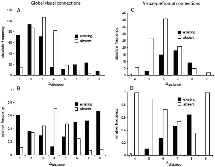
Frequency of corticocortical projections related to distance. (A,B) Absolute and (C,D) relative projection frequencies of global visual connections and visual prefrontal afferents, respectively. Relative frequencies represent the proportion of links of areas at a given distance that exist or are absent, out of all possible links at this distance.
Table 5. Rank-correlations of structural predictor variables and connection features of general visual and afferent prefrontal connections, based on the distribution of relative frequencies of existing and absent connections.
| Global visual connections | Visual prefrontal afferents | |||
|---|---|---|---|---|
| Predictor | Existence | Absence | Existence | Absence |
| Δdistance | ρ=0.27, p>0.05 | ρ=-0.41, p>0.05 | ρ=0.29, p>0.05 | ρ=-0.29, p>0.05 |
| Δthickness | ρ=-0.58, p<0.05 | ρ=0.62, p<0.05 | ρ=0.06, p>0.05 | ρ=-0.06, p>0.05 |
| Δtype | ρ=-0.96, p<0.00 | 1 ρ=0.96, p<0.001 | ρ=-0.93, p<0.05 | ρ=0.93, p<0.05 |
| Δdensity | ρ=-0.7, p>0.05 | ρ=0.7, p>0.05 | ρ=-0.90, p<0.05 | ρ=0.90, p<0.05 |
Similar properties are apparent for the dataset of projection neurons directed to prefrontal areas (Fig. 1C,D; Table 2). These data partially overlap with the data of Felleman and Van Essen (1991), focusing on projections from visual areas to different regions of the prefrontal cortex. Thus, these data partly correspond to the tail that is apparent in the data of Felleman and Van Essen (1991) for Δdistance > 4 borders (Fig. 1A,B). In particular, the relative frequency of visual-prefrontal projections (Fig. 1D) shows an increase in the proportion of existing projections from five to eight borders, which is opposite to what would be expected if connections are limited by distance. Overall, the correlation of Δdistance with the relative frequency of existing and absent visual-prefrontal connections is not significant (Table 5). Taken together, the analyses demonstrate that many connections exist between neighboring areas; however, there are also substantial numbers of connections linking areas over considerable distances, up to 8 borders. Therefore, distance may be a good predictor of the presence of connections at short distances, but appears to be a poor predictor for the absence of connections over long distances.
Structural type difference
Differences in structural type Δtype of cortical areas were previously shown to be predictive of laminar patterns of prefrontal connections in macaque monkeys (Barbas, 1986; Barbas and Rempel-Clower, 1997). The present analyses demonstrate that structural type differences are also closely correlated with the existence and absence of cortical projections. The majority of global visual (Fig. 2A) and visual-prefrontal (Fig. 2C) connections exist between areas that do not differ by more than two structural types. Moreover, the relative frequency of existing connections decreases, while the relative frequency of absent connections increases with Δtype (Fig. 2B,D). Both aspects of connections are significantly and strongly rank-correlated (|ρ|>0.9) with Δtype for global visual connections as well as visual-prefrontal afferents (Table 5). Therefore, the analyses generally demonstrate that structurally similar areas tend to be connected, while structurally dissimilar areas are not frequently connected.
Figure 2.
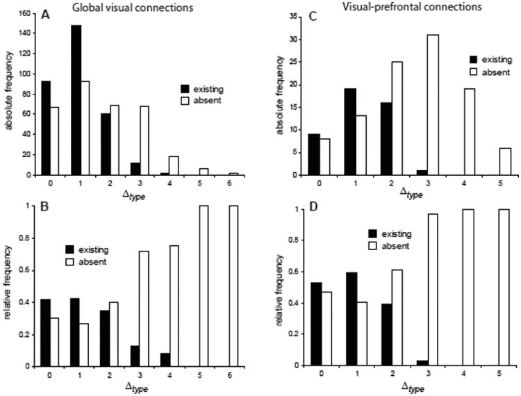
Frequency of corticocortical projections related to area type difference. Absolute (A,C) and relative (B, D) projection frequencies of global visual connections and visual prefrontal afferents, respectively. Relative frequencies represent the proportion of links of areas at a given type difference that exist or are absent, out of all possible links for such type differences.
Area neuronal density differences
Differences in the density of neurons in architectonic subdivisions of the lateral intraparietal (visuomotor) region were previously used as a quantitative measure of gradual type differences between cortical areas (Medalla and Barbas, 2006). Analyses of the relationship between neuronal density differences (Δdensity) and existence or absence of cortical connections yielded a similar picture as the correlation analysis of Δtype, to which Δdensity is related. The analyses indicated that the majority of global visual (Fig. 3A) as well as visual-prefrontal (Fig. 3C) connections exist between areas that do not differ in neuronal density by more than 20,000 neurons/mm3 (specifically, 64 of global visual and 88 of visual-prefrontal connections were found in this interval).
Figure 3.
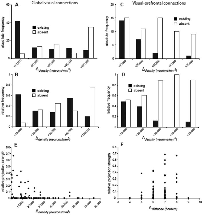
Frequency and strength of corticocortical projections related to area density difference. Absolute (A,C) and relative (B, D) projection frequencies of global visual connections and visual prefrontal afferents, respectively. Relative frequencies represent the proportion of existing or absent links of areas at a given interval of area density differences, out of all possible links. (E) Normalized projection strength (N%) of visual prefrontal afferents related to absolute area density difference. While areas of similar density may be linked strongly, areas of different densities tend not to be connected. (F) Normalized projection strength (N%) of visual prefrontal afferents related to border distance. In contrast to the decrease of projection strength with increasing difference in the neuronal density or type of cortical areas, projection strength increases with cortical distance, which is contrary to what would be expected if distance strictly limits the strength of cortical projections.
Moreover, the relative frequency of existing connections generally decreased with increasing neuronal density differences between areas, while the relative frequency of absent connections increased (with exceptions in the interval <40,000cells/mm3 for the global visual connections and the interval of <75,000cells/mm3 for the visual-prefrontal projections, Fig. 3B,D). The correlation of Δdensity with relative frequencies of existing and absent connections is high for the global visual as well as visual-prefrontal connections ((|ρ|>0.7), but reaches significance only for visual-prefrontal connections (Table 5).
Cortical thickness differences
Previous studies have posited that similarities in cortical thickness indicate an anatomical connection between similar areas. Thus, small Δthickness (differences in cortical thickness) should correspond to existing connections and larger Δthickness to absent connections between cortical areas. However, the distributions of absolute and relative frequencies of connections across thickness differences paint an inconsistent picture (Fig. 4A-D). While there is a moderate and significant tendency in the data of Felleman and Van Essen (1991) for smaller Δthickness to be associated with existing connections and larger Δthickness to be associated with absent connections (Fig. 4A,B), no such relation exists for the visual-prefrontal connections (Fig. 4C,D, Table 5).
Figure 4.
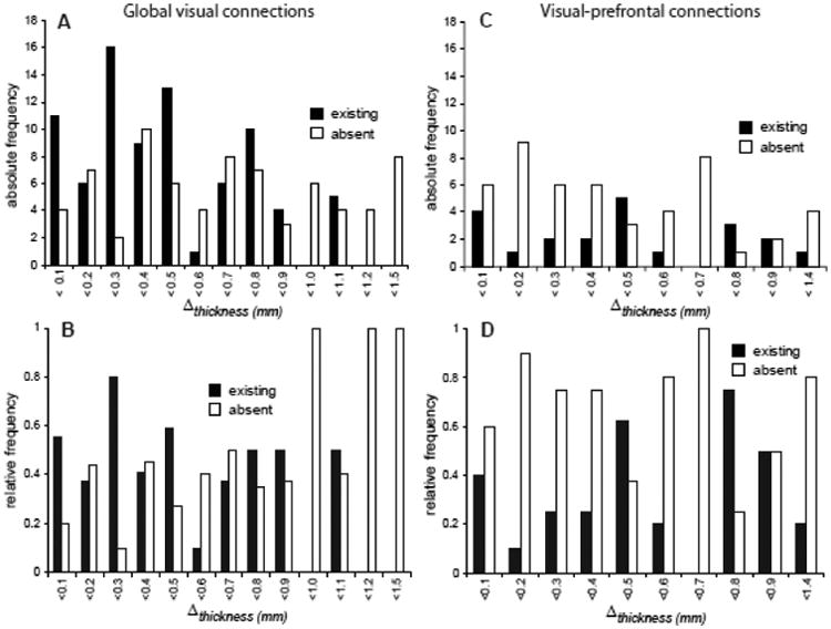
Frequency of corticocortical projections related to cortical thickness difference. Absolute (A,C) and relative (B, D) projection frequencies of global visual connections and visual prefrontal afferents, respectively. Relative frequencies represent the proportion of existing or absent links at a given interval of area thickness differences, out of all possible links.
Summary and partial correlations
The relations of the four structural parameters with existing and absent connections are summarized in Fig. 5. The figure panels demonstrate that existing connections are consistently associated with a smaller type difference or density difference between cortical areas than absent links, while such relations are not consistently found for distance or thickness differences.
Figure 5.
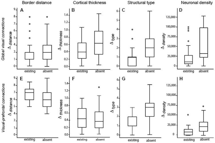
Summary of relations of structural parameters to global visual connections (top) and visual prefrontal afferents (bottom). Data are summarized by boxplots (showing median values as well as quartiles) to account for the ordinal nature of structural measures. While border distance (A) and cortical thickness differences (B) show contradictory relations in the two datasets, structural type difference (C) and neuronal density difference (D) consistently have the same relation with connection presence across the datasets. Particularly, the type difference or density difference of areas is smaller when areas are connected than when connections are absent.
We also tested if the marginal correlations reported above for individual structural parameters were reduced in partial correlations that took into account further variables. Of particular interest was whether the strong correlations seen for Δtype and Δdensity were reduced by controlling for Δdistance or Δthickness. We focused on the dataset for global visual connections (Felleman and Van Essen, 1991), since for the visual prefrontal dataset, Δdistance and Δthickness had only small marginal correlations with the presence of connections (Table 5).
Considering projections for which all corresponding variables existed, the correlations of Δtype and Δdensity with projection presence were only diminished by controlling for each other, as these variables are naturally linked, but not by controlling for Δdistance or Δthickness. For example, marginal correlation of Δtype: ρ=-0.59 (p<0.001); partial correlations controlling for Δdistance: ρ=-0.59 (p<0.001) or Δthickness: ρ=-0.54 (p<0.001). By contrast, the correlation for Δthickness (ρ=-0.29, p<0.001) was substantially reduced by controlling for Δtype (ρ=-0.11, p>0.05) or Δdensity (ρ=-0.18, p<0.05).
Projection strength
For the set of visual-prefrontal afferents, information on the relative projection strength, N%, of each connection was available. The plot of N% versus absolute Δdensity (Fig. 3E) confirms that connections rarely exist between areas that widely differ in neuronal density. Moreover, the plot demonstrates a trend of connections to be stronger when they link areas of similar neuronal density (rank correlation of absolute Δdensity with N%: ρ=-0.34, p<0.05). Similarly, connections were stronger when linking areas of similar architecture (rank correlation of absolute Δtype with N%: ρ=-0.49, p<0.001). By contrast, connection strength actually increased with distance (rank correlation of Δdistance with N%: ρ=0.29, p<0.05; Fig. 3F); while no correlation was seen with thickness differences (rank correlation absolute Δthickness with N%: ρ=0.04, p>0.05). Based on these findings, partial correlations were only calculated for the two meaningful predictors of absolute Δdensity and absolute Δtype. The correlation of absolute Δdensity with N% was strongly reduced when controlling for absolute Δtype (ρ=0.10, p>0.05), while the correlation of absolute Δtype with N% largely remained when controlling for absolute Δdensity (ρ=-0.40, p<0.001). This means that type differences account for a substantial portion of the correlation of projection strength with density differences, but not the other way around. This finding is consistent with the fact that neuronal density is an approximation of cortical type which also takes into account other structural factors as summarized in the Methods.
Laminar characteristics of projections: Qualitative patterns
Border distance and thickness difference
Qualitative laminar patterns were provided by the compilation of Felleman and Van Essen (1991), who classified connection origins and terminations into laminar categories (cf. Methods). Based on the laminar patterns, the authors also classified complete projections as ‘feedforward’ (FF), ‘feedback’ (FB) or ‘lateral’ (L), allowing for intermediate categories (i.e., FF/L, L/FB). Here, we rank-correlated the qualitative origin, termination and connection patterns with the four predictor variables (considering the laminar patterns in the order FF, FF/L, L, L/FB, FB).
The correlations of Δdistance or Δthickness demonstrated that these variables were moderately or weakly correlated with the laminar patterns (Table 6). In particular, distance showed no correlation with the laminar pattern of connections as reflected in their FF or FB type classification (Table 6).
Table 6. Rank correlations of structural parameters with laminar origins, terminations and projection profiles of visual projections.
Projection data are from Felleman and Van Essen (1991). |LB| indicates correlations of Δdistance with a symmetrical ordinal measure of the deviation of projections from a ‘lateral’ projection pattern (see Methods).
| Predictor | Origin patterns (S, S/B, B, B/I, I) | Termination patterns (M, M/C, C, C/F, F) | Projection type (FF, FF/L, L, L/FB, FB) |
|---|---|---|---|
| Δdistance | ρ=-0.26, p<0.001 | ρ=-0.14, p>0.05 | ρ=0.002, p>0.05 |
| ρ=0.29, p<0.001 (|LB|) | ρ=-0.06, p>0.05 (|LB|) | ρ=0.008, p>0.05 (|LB|) | |
| Δthickness | ρ=0.24, p>0.05 | ρ=-0.33, p<0.05 | ρ=0.29, p<0.05 |
| Δtype | ρ=-0.63, p<0.001 | ρ=0.76, p<0.001 | ρ=-0.76, p<0.001 |
| Δdensity | ρ=-0.71, p<0.001 | ρ=0.75, p<0.001 | ρ=-0.78, p<0.001 |
Structural type and neuronal density difference
Differences in structural type or neuronal density of visual cortical areas were closely correlated with the qualitative laminar connection patterns (Table 6). In particular, differences in cortical type were reflected in the projection categories of areas (Fig. 6), such that FF or FF/L connections were predominantly formed by projections from a higher type to a lower structural type, while FB or L/FB connections were formed by projections from lower to higher structural type. The largest number of L projections was seen for connections among the same types (Δtype=0). Strong and significant correlations with structural type differences were also observed for the patterns of origin and termination. Thus, pathways from higher to lower types originated predominantly in superficial layers (S), and terminated in the middle-deep cortical layers, including layer 4 (F), while projections from lower to higher types mostly had opposite patterns, originating in infragranular layers (I) and terminating outside layer 4 in the upper layers (M). Similar relationships were observed when structural differences between areas were quantified by the density difference, Δdensity (Table 6). Thus, the FF projection type is associated with a positive Δdensity (of 25,000 neurons/mm3 on average), and the FB type with a negative Δdensity, while projections with a ‘lateral’ component (FF/L or L/FB) link areas of comparable neuronal density (Fig. 6D).
Figure 6.
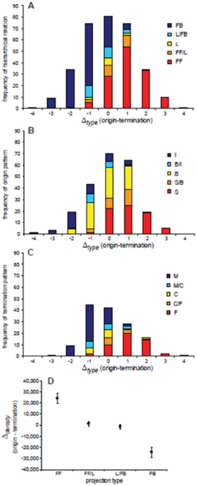
Type and density difference related to laminar patterns of global visual connections. (A) Overall direction of projections as classified by Felleman and Van Essen (1991) as FF, FF/L, L, FB/L, FB, related to area type differences. Projections of higher to lower type areas are typically FF, while projections of lower to higher type areas are FB. The largest number of L projections is formed between areas of the same type. Abbreviations: FF, ‘feedforward’; L, ‘lateral’; FB, ‘feedback’. (B) Laminar origins of projections, classified as I, B/I, B, S/B, S, related to area type differences. Abbreviations: I; ‘infragranular’; B, ‘bilaminar’; S, ‘supragranular’). (C) Laminar terminations of projections, classified as M, M/C, C, C/F, F, related to area type differences. Abbreviations: M, ‘multi layer avoiding layer 4’; C, ‘columnar’; F, ‘layer 4 predominant’ (Felleman and Van Essen, 1991). (D) Neuronal density differences of cortical areas related to the direction of projections between them. Projections that proceed from areas of greater to smaller density correspond to FF, while FB links project from areas with lower to areas with higher density of neurons. Projections with a lateral component proceed between areas of similar neuron density.
Laminar characteristics of projections: Quantitative origin patterns
Border distance and thickness difference
The datasets of Barbas (1986), Barone et al. (2000) and Markov et al. (2014) provide quantitative information on the laminar origin of visual-prefrontal projections, projections to visual areas V1 and V4, and projections from a large sample of visually responsive areas, respectively. Large NSG% values (close to 100) indicate a projection predominantly originating from upper cortical layers, while low NSG% (close to 0) is associated with predominantly deep layer projection origin, and NSG% around 50 indicates a projection of bilaminar (mixed upper and lower) origin.
Generally, correlation of the variables Δdistance and Δthickness with individual NSG% values led to inconsistent results when compared across the three analyzed datasets. While the correlations were substantial and significant for the projections to V1 and V4 (Barone et al., 2000), showing an inverse relation between the predictor variables and NSG% (Table 7), these relations were considerably weaker for the larger sample of general visual projections (Markov et al., 2014). Moreover, for the visual-prefontal projections (Table 2), the correlations were only moderate or weak and in the case of Δthickness not significant (Table 7).
Table 7. Rank correlations of structural parameters with quantitative patterns of laminar origins (NSG%).
For comparison, rank correlations were performed even when metric correlations were possible (i.e., for thickness and density differences).
| Predictor | V1 and V4 afferents Barone et al. (2000) | Global visual afferents Markov et al. (2014) | Visual prefrontal afferents (Table 2) |
|---|---|---|---|
| Δdistance | ρ=-0.57, p<0.05 | ρ=-0.02, p>0.05 | ρ=-0.32, p<0.05 |
| ρ=0.62, p<0.05 (|LB|) | ρ=0.12, p<0.05 (|LB|) | ρ=0.004, p>0.05 (|LB|) | |
| Δthickness | ρ=-0.75, p<0.001 | ρ=-0.41, p<0.001 | ρ=-0.19, p>0.05 |
| Δtype | ρ=0.93, p<0.001 | ρ= 0.51, p<0.001 | ρ=0.62, p<0.001 |
| Δdensity | ρ=0.89, p<0.001 | ρ= 0.45, p<0.001 | ρ=0.73, p<0.001 |
Note: |LB| indicates correlations of Δdistance with the symmetrical measure of normalized laminar bias, derived from NSG% (see Methods).
Type difference and neuronal density difference
Area type and neuronal density differences were significantly and moderately to strongly (ρ >0.45) correlated with the laminar origins of projections between the areas (Table 7). In particular, the analyses showed a positive correlation of Δtype and Δdensity with NSG%, such that projection neurons from areas of higher to lower type or higher to lower density mainly originated from the upper layers, and from lower to higher type or density mainly from the deep layers (Fig. 7). Projections between areas of similar type and density had a balanced bilaminar origin (NSG% around 50).
Figure 7.
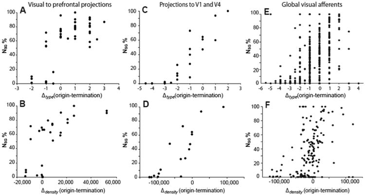
Relation of laminar projection origins to type differences and neuron density differences of cortical areas. (Top panels: A,C,E) Quantitative patterns of laminar origins depending on type difference. (Bottom panels: B,D,F) Quantitative patterns of laminar origins based on differences in neuron density between linked areas. In all three datasets (from left to right: prefrontal afferents, afferents of V1, V4 and global visual afferents), projection neurons from areas with higher density or higher type to areas with lower neuron density or lower type tend to originate from superficial layers, while projections from areas of lower type or sparser density to areas with higher neuron density or higher type originate from deep cortical layers.
We verified that these correlations were not substantially reduced when considering partial correlations that controlled for distance or differences in thickness. For example, for the dataset of V1 and V4 afferents (Barone et al., 2000), the partial correlation of NSG% with Δtype when controlling for Δdistance was ρ=0.90 (p<0.001), and the partial correlation of NSG% with Δtype controlling for Δthickness was ρ= 0.88 (p<0.001). By contrast, the partial correlations of NSG% with Δdistance when controlling for Δtype reduced to ρ= 0.15 (p>0.05) and with Δthickness when controlling for Δtype diminished to ρ=0.10 (P=0.7 p>0.05). Similarly, for the dataset of global visual afferents (Markov et al., 2014), the correlation of NSG% with Δtype or Δdensity were only mildly reduced when controlling for Δthickness (ρ=0.37, p<0.001 and ρ=0.32, p<0.001, respectively), while the correlation of NSG% with Δthickness disappeared when controlling for Δtype or Δdensity (ρ=-0.15, p>0.05 and ρ=-0.15, p>0.05, respectively.)
Correlations among predictive variables
In addition to considering partial correlations as described above, we also investigated general dependencies among the predictor variables.
In particular, for Dataset 1 (‘Global visual connections’, Felleman and Van Essen, 1991), the measures of Δdensity and Δtype are strongly correlated (ρ=0.93, p<0.001). Both measures are inversely correlated with thickness differences (ρ(Δdensity, Δthickness)=-0.67, p<0.001 and ρ(Δtype, Δthickness)=-0.61, p<0.001). By contrast, distance is not correlated with any of these measures (all |ρ|<0.01, all p>0.05).
For Dataset 2 (‘Visual prefrontal afferents’), the measures of Δdensity and Δtype are also strongly correlated (ρ=0.92, p<0.001). These measures are inversely related to distance (ρ(Δdensity, Δdistance)=-0.57, p<0.001 and ρ(Δtype, Δdistance)=-0.47, p<0.001) and are more weakly and inversely correlated with thickness differences (ρ(Δdensity, Δthickness)=-0.30, p<0.05 and ρ(Δtype, Δthickness)=-0.11, p>0.05), whereas distance is positively but weakly correlated with thickness differences (ρ =0.23, p<0.05).
Similarly, in Dataset 3 (‘V1 and V4 afferents’), type and density differences were also strongly correlated (ρ=0.96, p<0.001), and these measures were negatively correlated with thickness differences (ρ(Δdensity, Δthickness)=-0.87, p<0.001, ρ(Δtype, Δthickness)=-0.81, p<0.001) as well as with distance (ρ(Δdensity, Δdistance)=-0.67, p<0.05 and ρ(Δtype, Δdistance)=-0.66, p<0.001).
Finally, for Dataset 4 (‘Global visual afferents’, Markov et al., 2014), thickness differences were also negatively correlated with type differences (ρ=-0.59, p<0.001) as well as density differences (ρ=-0.64, p<0.001), but not significantly correlated with distance (ρ=0.08, p>0.05).
Therefore, the relationships among the structural variables across the analysed datasets are largely consistent. Differences in structural type and neuronal density of areas are strongly correlated, and negatively correlated with thickness differences. This relationship is due to the well known inverse relation between cortical type or density and area thickness (Economo, 1927).
Structural model of the primate visual system
Based on the observation that differences in structural type or neuron density of cortical areas are strongly correlated with the existence, absence and laminar features of connections between them, we created a structural diagram of the primate visual system. Here the areas are arranged by cortical type, with higher types at the outside and lower (more ‘limbic’) types towards the center of the diagram. In agreement with similar diagrams by Mesulam (1998) and Friston (2005), but in a departure from popular hierarchical arrangements (Felleman and Van Essen, 1991; Hilgetag et al., 2000c), the areas are arranged concentrically rather than sequentially. Interestingly, this arrangement also coincides with the intuitive placement of areas that are closer to the sensory periphery at the outside of the diagram. Connections are based on Felleman and Van Essen (1991) and colored in such a way that connections between areas of the same or adjacent type are shown in black, while links between areas differing by two types are shown in blue, and larger differences between connected areas are indicated by red links. The dominance of black connections underscores the consistency of the structural model.
Traditional hierarchical schemes of the primate visual system are further contrasted with the structural model in Fig. 9. Here, a spatial representation of an average hierarchy (Reid et al., 2009) derived from the sorting of areas by laminar projection patterns (Felleman and Van Essen, 1991; Hilgetag et al., 2000c) (Fig. 9A) is compared with the structural types of these areas (Fig. 9B). While there are some small apparent differences, the overall picture is very similar. This similarity derives from the observation in the present analyses that laminar patterns are closely and consistently tied to structural type differences. Thus, the type differences result in systematic laminar patterns of connection origins and terminations which in turn are reflected in the traditional hierarchical arrangements of visual areas.
Discussion
Overview
Using four extensive datasets of visual connections, we demonstrate that cortical structure and connections are closely linked. Structure is captured by a few salient parameters, including neuronal density and laminar structure distilled into a few cortical types seen throughout the cortical mantle (Barbas, 2015). Differences in these parameters between areas successfully predict essential connection features, including their presence or absence, density and laminar distribution of connection origins and terminations. By contrast, we found no coherent relations of connectivity with distance or thickness similarity. The absence of a consistent relationship with distance is in line with previous studies showing that the organization of mesoscopic projections in the primate brain does not appear to be strictly determined by wiring minimization principles (Kaiser and Hilgetag, 2006; Chen et al., 2013). Moreover, we found that similarities in cortical thickness were not consistently related to anatomical connections. This finding argues against the use of thickness similarities as a proxy for structural connectivity, as employed in several studies (e.g., He et al., 2007; Bassett et al., 2008; He et al., 2008; Liu et al., 2008; Bassett and Bullmore, 2009; He et al., 2009).
In general, our findings demonstrate that a structural model that has been derived and widely confirmed for connections of the primate prefrontal cortex (Barbas, 1986; Barbas and Rempel-Clower, 1997; Barbas et al., 2005a; Medalla and Barbas, 2006) applies to the presence and laminar patterns of visual cortical connections as well. This finding hints on general principles of mammalian cortical organization (Pandya et al., 1988; Hilgetag and Grant, 2010; Beul et al., 2014) and integrates long-range connections with local cortical architecture and intrinsic connectivity (Beul and Hilgetag, 2015).
Comparison of connection models
Cortical thickness was an unreliable predictor of cortical connections, which may not be surprising since thick gyral and thin sulcal parts of cortex often belong to the same architectonic area, as seen for prefrontal areas 8, 13, 46, among others. Each of these areas shows variable thickness due to cortical folding, but its sulcal and gyral parts have similar cellular features and connections (Hilgetag and Barbas, 2005; 2006).
Gradual changes in cortical structure often occur with distance (Pandya et al., 1988; Economo, 1927; Zilles and Amunts, 2012). For example, laminar structure is most distinctive in V1 and gradually blurs along an anterior direction, so that ventral visual cortices in the temporal pole have the fewest and least distinguishable layers (Pandya et al., 1988; Collins et al., 2010). However, the present analyses evaluated distance not only along the principal axes of architectonic gradients, but in all possible directions across the cortical sheet. This approach explains why distance and type difference of the studied areas were only mildly correlated, which allowed us to evaluate these parameters independently. To critically test these different models it is necessary to study connections of areas that have overall similar laminar structure but are distant from each other, or nearby areas with substantially different architecture, that is, cases, in which the two models make opposite predictions for the existence and laminar profiles of projections.
There are many examples of areas that are distant but strongly connected, such as prefrontal and temporal cortices. Moreover, these areas are connected in a laminar-specific manner. Thus, orbitofrontal areas 11 and 12, which have an intermediate eulaminate structure, innervate most robustly in a feedforward manner the middle layers of temporal dysgranular area 35 and the temporal pole, which have a poorly differentiated layer 4. In contrast, areas 11 and 12 target mostly the upper layers — in a feedback manner — the nearby inferior temporal cortices TE1-2, which have a better differentiated eulaminate structure (Rempel-Clower and Barbas, 2000). Similarly, lateral area 8 is strongly connected with the distantly situated intraparietal areas (LIPv, LIPd and 7a) (Medalla and Barbas, 2006). Even though both sets of areas are eulaminate (six-layer cortices), they differ somewhat by the sensitive parameter of neuronal density (Medalla and Barbas, 2006). Accordingly, caudal area 8 innervates robustly and primarily the upper layers of the comparatively denser LIPv area (feedback), but targets the middle-deep layers— in a feedforward manner— of the relatively less dense nearby parietal area 7a, as predicted by the structural model (Medalla and Barbas, 2006).
Limitations
Our analyses of the large database of Felleman and Van Essen (1991) were by necessity limited by the qualitative nature of the compiled data therein. We also had to abide by discrepancies in the data collected in different laboratories, such as the finding of a pathway in one study but not in another. In such cases we generally followed the assessment by Felleman and Van Essen (1991), but did not specifically distinguish between standard data and data marked as potentially less reliable. It was also necessary to use the maps of the cortical visual system that were available at that time and as described in the databases. Maps of the visual cortical system have since been supplemented by new areas and subdivisions of areas.
Defining the cortical type categories was initially based on qualitative criteria (Barbas, 1986; Barbas and Rempel-Clower, 1997) and more recently neuron density (Dombrowski et al., 2001). The choice of the number of categories was originally guided by studies that captured the changes seen in cortical structure in the prefrontal region (Barbas and Pandya, 1989; Dombrowski et al., 2001). The five types used for the prefrontal cortex allowed testing of hypotheses about the relationship of cortical structure and connection patterns (Barbas and Rempel-Clower, 1997). The current scheme consistently accommodated the five types used for the prefrontal region, but had to be extended by three additional types to allow for the greater laminar differentiation and higher neural density of some visual areas. As more indicators of cortical architecture are identified, it may be feasible to conduct multidimensional analyses of cortical structure and connectivity without qualitative categorization, and show where individual areas fall in a continuous, quantitative structural spectrum. Accordingly, analysis of several architectonic features yielded similar findings in the relative placement of uncategorized areas, and in their grouping into types (Medalla and Barbas, 2006).
Developmental events explain grades in architecture and connections
Differences in cortical structure are at the core of the structural model and an intriguing question is how they arise. We previously hypothesized that the graded differences in laminar architecture of cortical areas in adult primates suggest systematic differences in the duration of their development (Dombrowski et al. 2001; Barbas, 2015). According to our hypothesis, the fewer layers of limbic areas and lower density in the upper layers can be explained by a shorter developmental epoch, or selective loss of neurons during the regressive period of development. While there is a paucity of data on the latter, there exists some information on the former. Thus, whereas the onset of neurogenesis across cortices in macaque monkeys is nearly simultaneous (around E38-40), the end point is variable (Rakic, 2002; Lukaszewicz et al., 2006). Limbic areas have the shortest developmental period (end point at E70), while areas with progressively better laminar structure and higher neuronal density develop sequentially later, for instance, eulaminate area 11 at E80, A46 at E90, and V1 at E102 (Lukaszewicz et al., 2006), which also has more neurons than any other cortical area (O'Kusky and Colonnier, 1982). The high density of neurons in V1 is due to a shorter cell cycle duration than in V2, mediated by differential expression of cell cycle markers (Lukaszewicz et al., 2006).
The systematic structural variation in the cortex is further supported by graded expression of other neural markers along architectonic axes (Donoghue and Rakic, 1999; Zilles and Amunts, 2012). Within the cortical visual system, some markers are strongest in V1 and gradually attenuate through anterior parts of the ventral visual pathway (e.g., Occ1), while others are strongest at the opposite end and gradually diminish expression towards V1 (e.g., SPARC) (Takahata et al., 2009).
The linkage of the structural model to a graded pattern of developmental events extends its applicability to all cortical systems. And because areas develop their layers at different times (Lukaszewicz et al., 2006), the laminar pattern of connections is also graded (Barbas, 1986; Barbas and Rempel-Clower, 1997). Feedback connections, for example, link the deep layers of one cortex with layer 1 of another area. The deep layers are laid out first, according to the inside-out development of the cortex, and layer 1 is present at the onset of cortical development (Marín-Padilla, 1971). Genetic factors likely initiate cortical neurogenesis, but then self-organization takes over so that as areas develop they become connected. This principle can be expressed as “neurons that develop together wire together” (e.g., Barbas, 1986; Dombrowski et al., 2001). In addition to the graded pattern of laminar connections, the linkage of the structural model to developmental events also helps explain the presence and absence of connections, because areas that develop at the same time have comparable overall structure as well as a greater chance of being connected than dissimilar areas (Kaiser and Hilgetag, 2007). Additional evidence for this principle can be found at the cellular level in the neuronal wiring of the nematode C. elegans (Varier and Kaiser, 2011), as well as in computational simulations (Lim and Kaiser, 2015).
Functional implications of connection models
Traditional hierarchical schemes can be subsumed under the structural model, as shown in Figure 8. Despite its popularity, the hierarchical scheme of the visual system (Felleman and Van Essen, 1991), has not been successful in predicting functional properties of the system (Hegdé and Felleman, 2007). Three principal properties posited to be linked to hierarchy, namely latencies, receptive field size and complexity of responses, are poorly correlated with the proposed hierarchy.
Figure 8.
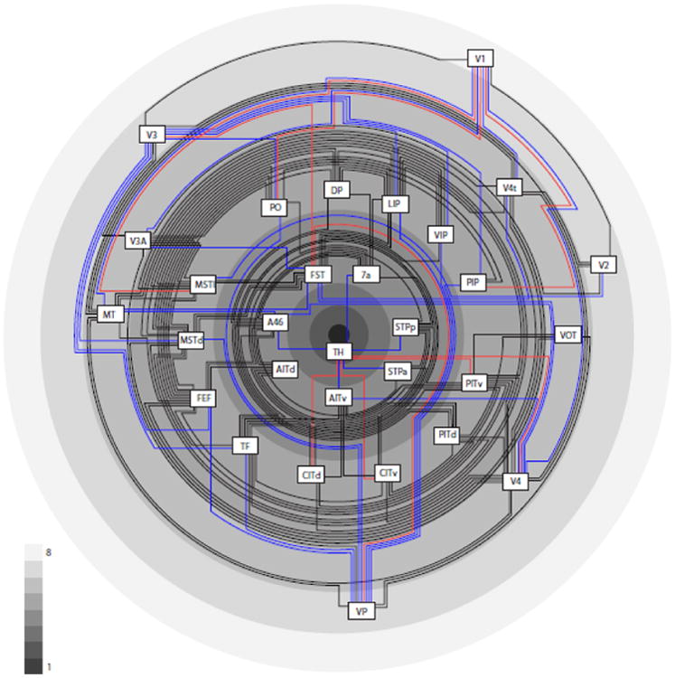
Structural model of the primate visual cortical system. Areas are arranged from higher types with dense, well-differentiated layers on the outer rings of the diagram proceeding to lower type areas on the inner rings of the scheme. Types are indicated by the shading of the rings, with lighter shading for higher and darker shading for lower types, as shown by the grey level scale. Connections (based on Felleman and Van Essen (1991)) between areas of the same or neighboring types are drawn in black, between areas separated by two types in blue, and projections between areas separated by more than two types are shown in red. The predominance of black projections indicates the consistency of the structural model.
The graded architecture of the cortex suggests a different organization, as depicted in Figure 9. This scheme places areas based on their structure and shows that connections depend on the structural differences between linked areas across the cortical landscape. The model thus takes distance and implied direction (‘forward’ or ‘backward’) out of the equation (Barbas and Rempel-Clower, 1997). How does the structural model fare with respect to latencies? For example, compared with some visual areas, latencies to visual stimuli in FEF are shorter in spite of its longer physical distance and hierarchical level from visual cortices (Schmolesky et al., 1998). The scheme of Felleman and Van Essen (1991) places FEF on the 8th processing level (out of 10). In contrast, the structural model (Fig. 8) positions FEF on the 4th structural level (out of 8), in line with its short latencies and based on its structural similarity with several dorsal stream areas that occupy the same ring in our model and are frequently interconnected. Thus, the structural model is more similar to topological sequences of the visual system that accurately predict onset latencies (Petroni et al., 2001) than the many-stage hierarchical arrangement of Felleman and Van Essen (1991).
Figure 9.
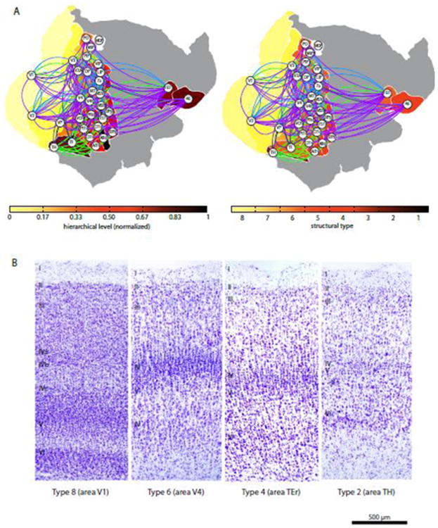
Comparison between average cortical hierarchy and structural types of the primate visual system. (A) Left, diagram adapted from Reid et al. (2009), right, structural types. While there are small apparent differences between these figures, the overall picture is quite similar. The present findings suggest that structural type differences are correlated with laminar projection patterns, and, thus, the structural type scheme underlies the hierarchical arrangement of areas resulting from the sorting of the oriented projections. (B) Coronal sections stained with Nissl show representative examples of cortical types. From left to right, note the decrease in the thickness and density of neurons in layer IV, the delineation of layers and lower density of neurons.
Moreover, the arrangement of areas within the structural model is closely aligned with sequences of areas derived from their spectral functional interactions (Bastos et al., 2015) Specifically, visual areas can be arranged by their pairwise interactions in the gamma and beta bands, and the strength of these interactions is correlated with the quantitative patterns of supragranular and infragranular projection origins, respectively (Bastos et al., 2015). The structural model, which was supported in the present study, implies that the laminar projection patterns are based on the graded structural differences of cortical areas, which means that there exists a mechanistic relationship between the structural differences of cortical areas and their communication in different frequency channels. By extension, this observation suggests that a structural characterization of cortices may also help predict their functional interactions in the human brain.
The structural model places limbic cortices at the center of cortical organization which are also the ultimate feedback systems by virtue of their widespread connection origin in the deep layers and termination in the upper layers of association cortices (Barbas, 1986; Barbas and Rempel-Clower, 1997). We had previously hypothesized that this pattern suggests that limbic areas have a tonic influence on the neuraxis (Barbas, 1995; 2000), recently substantiated by their wide involvement in ‘default mode networks’ (Raichle, 2011). The simple laminar architecture of limbic areas (Beul and Hilgetag, 2015), their low myelin content, presence of developmentally regulated proteins for axon growth and branching in adult primates suggests high mutability that allows flexible behavior (Dombrowski et al., 2001; Zikopoulos and Barbas, 2010).
At the level of layers, the origin and termination of connections occur within microenvironments populated by distinct classes of inhibitory neurons, which also show specific laminar distributions. The superimposition of the graded laminar pattern of connections and functional classes of inhibitory neurons (Bunce and Barbas, 2011; Bunce et al., 2013; Anderson et al., 2015) provides the framework to model shifts in cortical rhythms (Lakatos et al., 2008; Ainsworth et al., 2012) for flexible behavior. The structural model can also be used to hypothesize specific disruptions in disease. For example, dysgranular area 32 in the anterior cingulate sends a pathway from neurons mostly in the deep layers, whose axons terminate most robustly in the upper layers (1-3a) of lateral eulaminate prefrontal areas (e.g., Barbas, 1986; Barbas and Pandya, 1989; Barbas et al., 1999), consistent with the structural model for connections (Barbas and Rempel-Clower, 1997). Detailed analysis of the termination of axons from area 32 to lateral prefrontal area 9 or 46 showed that, when axons innervate inhibitory neurons, their primary targets are calbindin inhibitory neurons (Medalla and Barbas, 2009; 2010). Other studies have shown that calbindin inhibitory neurons are synaptically suited to reduce noise and enhance signals in working memory tasks in lateral prefrontal cortices (Wang et al., 2004). Interestingly, there is a decrease of pyramidal neurons in the deep layers of the anterior cingulate area in schizophrenia (Benes et al., 2001). Based on the predictions of the structural model, and empirical data on connections in non-human primates, the pathway from anterior cingulate cortex to lateral prefrontal cortex could be weakened in schizophrenia. This prediction is consistent with the distractibility in schizophrenia, which is at the core of the cognitive deficit in the disease.
In contrast, there is an increase in the density of medium and thin axons in the superficial white matter below the anterior cingulate cortex (area 32) in the brains of adults with autism (Zikopoulos and Barbas, 2010; 2013). Fibers in the superficial white matter of the anterior cingulate project to nearby areas, including lateral prefrontal cortices. The higher density of axons that extend over short or medium distances just below anterior cingulate area 32 in autism would have the opposite effect on lateral prefrontal areas than in schizophrenia: strengthening of a pathway to lateral prefrontal areas, shown to be suited to reduce noise and enhance signal in primates. This evidence may help explain the ability of individuals with autism to focus intensely on a stimulus, but also lose flexibility to refocus attention when needed (Medalla and Barbas, 2009; 2010; Zikopoulos and Barbas, 2010; 2013). The structural model, thus, has broad implications for the organization of the cortex, its development, and the recruitment of cortical areas in behavior, as suggested for neurocognitive maps in primates (Mesulam, 2008) and disruption in psychiatric and neurologic diseases. From the combination of these features, one may begin to derive generic models of cortical organization.
Highlights.
Comparison of models for cortical connections
Analysis of extensive connectivity data of the macaque visual system
Cortical type and density relate to connection existence and laminar patterns
Distance and cortical thickness relate less consistently to connections
The findings strongly support a structural model of cortical connectivity
Acknowledgments
CCH and SB were supported by DFG Collaborative Research Center Grant SFB 936/A1. CCH was also supported by DFG Collaborative Research Center Grant TRR 169/A2. MM was supported by NIMH (National Institute of Mental Health) grant K99 MH101234. HB was supported by grants from NIH (NINDS R01NS024760; and NIMH, R01MH057414) and CELEST, an NSF Science of Learning Center (NSF OMA-0835976).
Footnotes
Conflict of Interest: The authors declare no competing financial interests.
Publisher's Disclaimer: This is a PDF file of an unedited manuscript that has been accepted for publication. As a service to our customers we are providing this early version of the manuscript. The manuscript will undergo copyediting, typesetting, and review of the resulting proof before it is published in its final citable form. Please note that during the production process errors may be discovered which could affect the content, and all legal disclaimers that apply to the journal pertain.
References
- Ainsworth M, Lee S, Cunningham MO, Traub RD, Kopell NJ, Whittington MA. Rates and rhythms: a synergistic view of frequency and temporal coding in neuronal networks. Neuron. 2012;75:572–583. doi: 10.1016/j.neuron.2012.08.004. [DOI] [PubMed] [Google Scholar]
- Anderson MC, Bunce JG, Barbas H. Prefrontal-hippocampal pathways underlying inhibitory control over memory. Neurobiol Learn Mem. 2015 Nov 28; doi: 10.1016/j.nlm.2015.11.008. [DOI] [PMC free article] [PubMed] [Google Scholar]
- Barbas H. Pattern in the laminar origin of corticocortical connections. J Comp Neurol. 1986;252:415–422. doi: 10.1002/cne.902520310. [DOI] [PubMed] [Google Scholar]
- Barbas H. Anatomic organization of basoventral and mediodorsal visual recipient prefrontal regions in the rhesus monkey. J Comp Neurol. 1988;276:313–342. doi: 10.1002/cne.902760302. [DOI] [PubMed] [Google Scholar]
- Barbas H. Organization of cortical afferent input to orbitofrontal areas in the rhesus monkey. Neuroscience. 1993;56:841–864. doi: 10.1016/0306-4522(93)90132-y. [DOI] [PubMed] [Google Scholar]
- Barbas H. Anatomic basis of cognitive-emotional interactions in the primate prefrontal cortex. Neurosci Biobehav R. 1995;19:499–510. doi: 10.1016/0149-7634(94)00053-4. [DOI] [PubMed] [Google Scholar]
- Barbas H. Connections underlying the synthesis of cognition, memory, and emotion in primate prefrontal cortices. Brain Res Bull. 2000;52:319–330. doi: 10.1016/s0361-9230(99)00245-2. [DOI] [PubMed] [Google Scholar]
- Barbas H. General Cortical and Special Prefrontal Connections: Principles from Structure to Function. Annu Rev Neurosci. 2015;38:269–289. doi: 10.1146/annurev-neuro-071714-033936. [DOI] [PubMed] [Google Scholar]
- Barbas H, García-Cabezas MÁ. Motor cortex layer 4: less is more. Trends Neurosci. 2015;38:259–61. doi: 10.1016/j.tins.2015.03.005. 2015. [DOI] [PMC free article] [PubMed] [Google Scholar]
- Barbas H, Hilgetag CC, Saha S, Dermon CR, Suski JL. Parallel organization of contralateral and ipsilateral prefrontal cortical projections in the rhesus monkey. BMC Neurosci. 2005a;6:32. doi: 10.1186/1471-2202-6-32. [DOI] [PMC free article] [PubMed] [Google Scholar]
- Barbas H, Medalla M, Alade O, Suski J, Zikopoulos B, Lera P. Relationship of prefrontal connections to inhibitory systems in superior temporal areas in the rhesus monkey. Cereb Cortex. 2005b;15:1356–1370. doi: 10.1093/cercor/bhi018. [DOI] [PubMed] [Google Scholar]
- Barbas H, Mesulam MM. Organization of Afferent Input to Subdivisions of Area-8 in the Rhesus-Monkey. J Comp Neurol. 1981;200:407–431. doi: 10.1002/cne.902000309. [DOI] [PubMed] [Google Scholar]
- Barbas H, Pandya D. Architecture and Intrinsic Connections of the Prefrontal Cortex in the Rhesus-Monkey. J Comp Neurol. 1989;286:353–375. doi: 10.1002/cne.902860306. [DOI] [PubMed] [Google Scholar]
- Barbas H, Rempel-Clower N. Cortical structure predicts the pattern of corticocortical connections. Cereb Cortex. 1997;7:635–646. doi: 10.1093/cercor/7.7.635. [DOI] [PubMed] [Google Scholar]
- Barone P, Batardiere A, Knoblauch K, Kennedy H. Laminar distribution of neurons in extrastriate areas projecting to visual areas V1 and V4 correlates with the hierarchical rank and indicates the operation of a distance rule. J Neurosci. 2000;20:3263–3281. doi: 10.1523/JNEUROSCI.20-09-03263.2000. [DOI] [PMC free article] [PubMed] [Google Scholar]
- Bassett DS, Bullmore E, Verchinski BA, Mattay VS, Weinberger DR, Meyer-Lindenberg A. Hierarchical organization of human cortical networks in health and schizophrenia. J Neurosci. 2008;28:9239–9248. doi: 10.1523/JNEUROSCI.1929-08.2008. [DOI] [PMC free article] [PubMed] [Google Scholar]
- Bassett DS, Bullmore ET. Human brain networks in health and disease. Curr Opin Neurol. 2009;22:340–347. doi: 10.1097/WCO.0b013e32832d93dd. [DOI] [PMC free article] [PubMed] [Google Scholar]
- Bastos AM, Vezoli J, Bosman CA, Schoffelen JM, Oostenveld R, Dowdall JR, De Weerd P, Kennedy H, Fries P. Visual Areas Exert Feedforward and Feedback Influences through Distinct Frequency Channels. Neuron. 2015;85:390–401. doi: 10.1016/j.neuron.2014.12.018. [DOI] [PubMed] [Google Scholar]
- Benes FM, Vincent SL, Todtenkopf M. The density of pyramidal and nonpyramidal neurons in anterior cingulate cortex of schizophrenic and bipolar subjects. Biol Psychiatry. 2001;50:395–406. doi: 10.1016/s0006-3223(01)01084-8. [DOI] [PubMed] [Google Scholar]
- Beul SF, Grant S, Hilgetag CC. A predictive model of the cat cortical connectome based on cytoarchitecture and distance. Brain Struct Funct. 2014 doi: 10.1007/s00429-014-0849-y. [DOI] [PMC free article] [PubMed] [Google Scholar]
- Beul SF, Hilgetag CC. Towards a “canonical” agranular cortical microcircuit. Front Neuroanat. 2015;8 doi: 10.3389/fnana.2014.00165. [DOI] [PMC free article] [PubMed] [Google Scholar]
- Boussaoud D, Desimone R, Ungerleider LG. Visual topography of area TEO in the macaque. J Comp Neurol. 1991;306:554–575. doi: 10.1002/cne.903060403. [DOI] [PubMed] [Google Scholar]
- Bullier J, Nowak LG. Parallel versus serial processing: new vistas on the distributed organization of the visual system. Current Opinion in Neurobiology. 1995;5:497–503. doi: 10.1016/0959-4388(95)80011-5. [DOI] [PubMed] [Google Scholar]
- Bullmore E, Sporns O. Complex brain networks: graph theoretical analysis of structural and functional systems. Nat Rev Neurosci. 2009;10:186–198. doi: 10.1038/nrn2575. [DOI] [PubMed] [Google Scholar]
- Bunce JG, Barbas H. Prefrontal pathways target excitatory and inhibitory systems in memory-related medial temporal cortices. NeuroImage. 2011;55:1461–1474. doi: 10.1016/j.neuroimage.2011.01.064. [DOI] [PMC free article] [PubMed] [Google Scholar]
- Bunce JG, Zikopoulos B, Feinberg M, Barbas H. Parallel prefrontal pathways reach distinct excitatory and inhibitory systems in memory-related rhinal cortices. J Comp Neurol. 2013;521:4260–4283. doi: 10.1002/cne.23413. [DOI] [PMC free article] [PubMed] [Google Scholar]
- Chen Y, Wang S, Hilgetag CC, Zhou C. Trade-off between Multiple Constraints Enables Simultaneous Formation of Modules and Hubs in Neural Systems. PLoS Comput Biol. 2013;9(3):e1002937. doi: 10.1371/journal.pcbi.1002937. [DOI] [PMC free article] [PubMed] [Google Scholar]
- Collins CE, Airey DC, Young NA, Leitch DB, Kaas JH. Neuron densities vary across and within cortical areas in primates. Proc Natl Acad Sci USA. 2010;107:15927–15932. doi: 10.1073/pnas.1010356107. [DOI] [PMC free article] [PubMed] [Google Scholar]
- Ding SL, Van Hoesen GW. Borders, extent, and topography of human perirhinal cortex as revealed using multiple modern neuroanatomical and pathological markers. Hum Brain Mapp. 2010;31:1359–1379. doi: 10.1002/hbm.20940. [DOI] [PMC free article] [PubMed] [Google Scholar]
- Dombrowski SM, Hilgetag CC, Barbas H. Quantitative architecture distinguishes prefrontal cortical systems in the rhesus monkey. Cereb Cortex. 2001;11:975–988. doi: 10.1093/cercor/11.10.975. [DOI] [PubMed] [Google Scholar]
- Donoghue MJ, Rakic P. Molecular gradients and compartments in the embryonic primate cerebral cortex. Cereb Cortex. 1999;9:586–600. doi: 10.1093/cercor/9.6.586. [DOI] [PubMed] [Google Scholar]
- Economo Von CF. Zellaufbau der Grosshirnrinde des Menschen. Berlin: Springer; 1927. [Google Scholar]
- Ercsey-Ravasz M, Markov NT, Lamy C, Van Essen DC, Knoblauch K, Toroczkai Z, Kennedy H. A predictive network model of cerebral cortical connectivity based on a distance rule. Neuron. 2013;80:184–197. doi: 10.1016/j.neuron.2013.07.036. [DOI] [PMC free article] [PubMed] [Google Scholar]
- Felleman DJ, Van Essen DC. Distributed hierarchical processing in the primate cerebral cortex. Cereb Cortex. 1991;1:1–47. doi: 10.1093/cercor/1.1.1-a. [DOI] [PubMed] [Google Scholar]
- Floyd RW. Algorithm 97: Shortest path. Commun Acm. 1962;5:345. [Google Scholar]
- Friston K. A theory of cortical responses. Philos T Roy Soc B. 2005;360:815–836. doi: 10.1098/rstb.2005.1622. [DOI] [PMC free article] [PubMed] [Google Scholar]
- García-Cabezas MÁ, Barbas H. Area 4 has layer IV in adult primates. Eur J Neurosci. 2014;39:1824–34. doi: 10.1111/ejn.12585. [DOI] [PMC free article] [PubMed] [Google Scholar]
- Grant S, Hilgetag CC. Graded classes of cortical connections: quantitative analyses of laminar projections to motion areas of cat extrastriate cortex. Eur J Neurosci. 2005;22:681–696. doi: 10.1111/j.1460-9568.2005.04232.x. [DOI] [PMC free article] [PubMed] [Google Scholar]
- Gundersen HJ, Bagger P, Bendtsen TF, Evans SM, Korbo L, Marcussen N, Møller A, Nielsen K, Nyengaard JR, Pakkenberg B, et al. The new stereological tools: disector, fractionator, nucleator and point sampled intercepts and their use in pathological research and diagnosis. APMIS. 1988;96:857–881. doi: 10.1111/j.1699-0463.1988.tb00954.x. [DOI] [PubMed] [Google Scholar]
- He Y, Chen ZJ, Evans AC. Small-world anatomical networks in the human brain revealed by cortical thickness from MRI. Cereb Cortex. 2007;17:2407–2419. doi: 10.1093/cercor/bhl149. [DOI] [PubMed] [Google Scholar]
- He Y, Chen Z, Evans A. Structural insights into aberrant topological patterns of large-scale cortical networks in Alzheimer's disease. J Neurosci. 2008;28:4756–4766. doi: 10.1523/JNEUROSCI.0141-08.2008. [DOI] [PMC free article] [PubMed] [Google Scholar]
- He Y, Dagher A, Chen Z, Charil A, Zijdenbos A, Worsley K, Evans A. Impaired small-world efficiency in structural cortical networks in multiple sclerosis associated with white matter lesion load. Brain. 2009;132:3366–3379. doi: 10.1093/brain/awp089. [DOI] [PMC free article] [PubMed] [Google Scholar]
- Hegdé J, Felleman DJ. Reappraising the functional implications of the primate visual anatomical hierarchy. The Neuroscientist. 2007;13:416–421. doi: 10.1177/1073858407305201. [DOI] [PubMed] [Google Scholar]
- Hilgetag CC, Barbas H. Developmental mechanics of the primate cerebral cortex. Anatomy and Embryology. 2005;210:411–417. doi: 10.1007/s00429-005-0041-5. [DOI] [PubMed] [Google Scholar]
- Hilgetag CC, Barbas H. Role of mechanical factors in the morphology of the primate cerebral cortex. PLoS Comput Biol. 2006;2:e22. doi: 10.1371/journal.pcbi.0020022. [DOI] [PMC free article] [PubMed] [Google Scholar]
- Hilgetag CC, Burns GAPC, O'Neill MA, Scannell JW, Young MP. Anatomical connectivity defines the organization of clusters of cortical areas in the macaque and the cat. Philos T Roy Soc B. 2000a;355:91–110. doi: 10.1098/rstb.2000.0551. [DOI] [PMC free article] [PubMed] [Google Scholar]
- Hilgetag CC, Dombrowski SM, Barbas H. Classes and gradients of prefrontal cortical organization in the primate. Neurocomputing. 2002;44-46:823–829. [Google Scholar]
- Hilgetag CC, Grant S. Cytoarchitectural differences are a key determinant of laminar projection origins in the visual cortex. NeuroImage. 2010;51:1006–1017. doi: 10.1016/j.neuroimage.2010.03.006. [DOI] [PubMed] [Google Scholar]
- Hilgetag CC, Grant S. Uniformity, specificity and variability of corticocortical connectivity. Philos T Roy Soc B. 2000b;355:7–20. doi: 10.1098/rstb.2000.0546. [DOI] [PMC free article] [PubMed] [Google Scholar]
- Hilgetag CC, Medalla M, Barbas H. Relationship of connection patterns to the architecture of the primate visual cortex. Soc Neurosci Abstr. 2008;34:215.2. [Google Scholar]
- Hilgetag CC, O'Neill MA, Young MP. Indeterminate organization of the visual system. Science. 1996;271:776–777. doi: 10.1126/science.271.5250.776. [DOI] [PubMed] [Google Scholar]
- Hilgetag CC, O'Neill MA, Young MP. Hierarchical organization of macaque and cat cortical sensory systems explored with a novel network processor. Philos T Roy Soc B. 2000c;355:71–89. doi: 10.1098/rstb.2000.0550. [DOI] [PMC free article] [PubMed] [Google Scholar]
- Howard CV, Reed MG. Unbiased Stereology, Three-dimensional Measurement in Microscopy. BIOS Scientific Publishers Limited; Oxford: 1998. [Google Scholar]
- Hyvarinen J. Regional Distribution of Functions in Parietal Association Area 7 of the Monkey. Brain Res. 1981;206:287–303. doi: 10.1016/0006-8993(81)90533-3. [DOI] [PubMed] [Google Scholar]
- Kaiser M, Hilgetag CC. Nonoptimal component placement, but short processing paths, due to long-distance projections in neural systems. PLoS Comput Biol. 2006;2:e95. doi: 10.1371/journal.pcbi.0020095. [DOI] [PMC free article] [PubMed] [Google Scholar]
- Kaiser M, Hilgetag CC. Development of multi-cluster cortical networks by time windows for spatial growth. Neurocomputing. 2007;70:1829–1832. [Google Scholar]
- Kaiser M, Hilgetag CC, van Ooyen A. A simple rule for axon outgrowth and synaptic competition generates realistic connection lengths and filling fractions. Cerebral Cortex. 2009;19:3001–3010. doi: 10.1093/cercor/bhp071. [DOI] [PubMed] [Google Scholar]
- Klyachko VA, Stevens CF. Connectivity optimization and the positioning of cortical areas. Proc Natl Acad Sci USA. 2003;100:7937–7941. doi: 10.1073/pnas.0932745100. [DOI] [PMC free article] [PubMed] [Google Scholar]
- Lakatos P, Karmos G, Mehta AD, Ulbert I, Schroeder CE. Entrainment of Neuronal Oscillations as a Mechanism of Attentional Selection. Science. 2008;320:110–113. doi: 10.1126/science.1154735. [DOI] [PubMed] [Google Scholar]
- Lerch JP, Worsley K, Shaw WP, Greenstein DK, Lenroot RK, Giedd J, Evans AC. Mapping anatomical correlations across cerebral cortex (MACACC) using cortical thickness from MRI. NeuroImage. 2006;31:993–1003. doi: 10.1016/j.neuroimage.2006.01.042. [DOI] [PubMed] [Google Scholar]
- Liu Y, Liang M, Zhou Y, He Y, Hao Y, Song M, Yu C, Liu H, Liu Z, Jiang T. Disrupted small-world networks in schizophrenia. Brain. 2008;131:945–961. doi: 10.1093/brain/awn018. [DOI] [PubMed] [Google Scholar]
- Lukaszewicz A, Cortay V, Giroud P, Berland M, Smart I, Kennedy H, Dehay C. The concerted modulation of proliferation and migration contributes to the specification of the cytoarchitecture and dimensions of cortical areas. Cereb Cortex. 2006;16 Suppl 1:i26–i34. doi: 10.1093/cercor/bhk011. [DOI] [PubMed] [Google Scholar]
- MacNeil MA, Lomber SG, Payne BR. Thalamic and cortical projections to middle suprasylvian cortex of cats: constancy and variation. Exp Brain Res. 1997;114:24–32. doi: 10.1007/pl00005620. [DOI] [PubMed] [Google Scholar]
- Marín Padilla M. Early prenatal ontogenesis of the cerebral cortex (neocortex) of the cat (Felis domestica). A Golgi study. I The primordial neocortical organization. Z Anat Entwicklungsgesch. 1971;134:117–145. doi: 10.1007/BF00519296. [DOI] [PubMed] [Google Scholar]
- Markov NT, Ercsey-Ravasz M, Lamy C, Ribeiro Gomes AR, Magrou L, Misery P, Giroud P, Barone P, Dehay C, Toroczkai Z, Knoblauch K, Van Essen DC, Kennedy H. The role of long-range connections on the specificity of the macaque interareal cortical network. Proceedings of the National Academy of Sciences. 2013;110:5187–5192. doi: 10.1073/pnas.1218972110. [DOI] [PMC free article] [PubMed] [Google Scholar]
- Markov NT, Misery P, Falchier A, Lamy C, Vezoli J, Quilodran R, Gariel MA, Giroud P, Ercsey-Ravasz M, Pilaz LJ, Huissoud C, Barone P, Dehay C, Toroczkai Z, Van Essen DC, Kennedy H, Knoblauch K. Weight consistency specifies regularities of macaque cortical networks. Cerebral Cortex. 2011;21:1254–1272. doi: 10.1093/cercor/bhq201. [DOI] [PMC free article] [PubMed] [Google Scholar]
- Markov NT, Vezoli J, Chameau P, Falchier A, Quilodran R, Huissoud C, Lamy C, Misery P, Giroud P, Ullman S, Barone P, Dehay C, Knoblauch K, Kennedy H. Anatomy of hierarchy: feedforward and feedback pathways in macaque visual cortex. J Comp Neurol. 2014;522:225–259. doi: 10.1002/cne.23458. [DOI] [PMC free article] [PubMed] [Google Scholar]
- Medalla M, Barbas H. Diversity of laminar connections linking periarcuate and lateral intraparietal areas depends on cortical structure. Eur J Neurosci. 2006;23:161–179. doi: 10.1111/j.1460-9568.2005.04522.x. [DOI] [PubMed] [Google Scholar]
- Medalla M, Barbas H. Synapses with inhibitory neurons differentiate anterior cingulate from dorsolateral prefrontal pathways associated with cognitive control. Neuron. 2009;61:609–620. doi: 10.1016/j.neuron.2009.01.006. [DOI] [PMC free article] [PubMed] [Google Scholar]
- Medalla M, Barbas H. Anterior cingulate synapses in prefrontal areas 10 and 46 suggest differential influence in cognitive control. J Neurosci. 2010;30:16068–16081. doi: 10.1523/JNEUROSCI.1773-10.2010. [DOI] [PMC free article] [PubMed] [Google Scholar]
- Mesulam M. Representation, Inference, and Transcendent Encoding in Neurocognitive Networks of the Human Brain. Ann Neurol. 2008;64:367–378. doi: 10.1002/ana.21534. [DOI] [PubMed] [Google Scholar]
- Mesulam MM. From sensation to cognition. Brain. 1998;121(Pt 6):1013–1052. doi: 10.1093/brain/121.6.1013. [DOI] [PubMed] [Google Scholar]
- Neal JW, Pearson RC, Powell TP. The cortico-cortical connections within the parieto-temporal lobe of area PG,7a, in the monkey. Brain Res. 1988;438:343–350. doi: 10.1016/0006-8993(88)91361-3. [DOI] [PubMed] [Google Scholar]
- O'Kusky J, Colonnier M. A laminar analysis of the number of neurons, glia, and synapses in the visual cortex (area 17) of adult macaque monkeys. J Comp Neurol. 1982;210:278–290. doi: 10.1002/cne.902100307. [DOI] [PubMed] [Google Scholar]
- Pandya DN, Seltzer B, Barbas H. Input-output organization of the primate cerebral cortex. In Comparative Primate Biology. In: Steklis HD, Erwin J, editors. Neurosciences. Vol. 4. New York: Alan R.Liss; 1988. pp. 39–80. [Google Scholar]
- Petroni F, Panzeri S, Hilgetag CC, Kötter R, Young MP. Simultaneity of responses in a hierarchical visual network. Neuroreport. 2001;12:2753–2759. doi: 10.1097/00001756-200108280-00032. [DOI] [PubMed] [Google Scholar]
- Raichle M. The restless brain. Brain Connectivity. 2011;1 doi: 10.1089/brain.2011.0019. [DOI] [PMC free article] [PubMed] [Google Scholar]
- Rakic P. Neurogenesis in adult primate neocortex: an evaluation of the evidence. Nat Rev Neurosci. 2002;3:65–71. doi: 10.1038/nrn700. [DOI] [PubMed] [Google Scholar]
- Reid AT, Krumnack A, Wanke E, Kötter R. Optimization of cortical hierarchies with continuous scales and ranges. NeuroImage. 2009;47:611–617. doi: 10.1016/j.neuroimage.2009.04.061. [DOI] [PubMed] [Google Scholar]
- Rempel-Clower NL, Barbas H. The laminar pattern of connections between prefrontal and anterior temporal cortices in the Rhesus monkey is related to cortical structure and function. Cereb Cortex. 2000;10:851–865. doi: 10.1093/cercor/10.9.851. [DOI] [PubMed] [Google Scholar]
- Saleem KS, Price JL, Hashikawa T. Cytoarchitectonic and chemoarchitectonic subdivisions of the perirhinal and parahippocampal cortices in macaque monkeys. J Comp Neurol. 2007;500:973–1006. doi: 10.1002/cne.21141. [DOI] [PubMed] [Google Scholar]
- Scannell JW, Grant S, Payne BR, Baddeley R. On Variability in the Density of Corticocortical and Thalamocortical Connections. Philos T Roy Soc B. 2000;355:21–35. doi: 10.1098/rstb.2000.0547. [DOI] [PMC free article] [PubMed] [Google Scholar]
- Schall JD, Morel A, King DJ, Bullier J. Topography of visualcortex connections with frontal eye field in macaque: Convergence andsegregation of processing streams. J Neurosci. 1995;15:4464–4487. doi: 10.1523/JNEUROSCI.15-06-04464.1995. [DOI] [PMC free article] [PubMed] [Google Scholar]
- Schmitz C, Hof PR. Design-based stereology in neuroscience. Neuroscience. 2005;130:813–831. doi: 10.1016/j.neuroscience.2004.08.050. [DOI] [PubMed] [Google Scholar]
- Schmolesky MT, Wang Y, Hanes DP, Thompson KG, Leutgeb S, Schall JD, Leventhal AG. Signal timing across the macaque visual system. J Neurophysiol. 1998;79:3272–3278. doi: 10.1152/jn.1998.79.6.3272. [DOI] [PubMed] [Google Scholar]
- Scholtens LH, Schmidt R, de Reus MA, van den Heuvel MP. Linking macroscale graph analytical organization to microscale neuroarchitectonics in the macaque connectome. J Neurosci. 2014;34:12192–12205. doi: 10.1523/JNEUROSCI.0752-14.2014. [DOI] [PMC free article] [PubMed] [Google Scholar]
- Seltzer B, Pandya DN. Converging visual and somatic sensory cortical input to the intraparietal sulcus of the rhesus monkey. Brain Res. 1980;192:339–51. doi: 10.1016/0006-8993(80)90888-4. [DOI] [PubMed] [Google Scholar]
- Sporns O. Networks of the Brain. MIT Press; 2010. [Google Scholar]
- Sporns O, Chialvo DR, Kaiser M, Hilgetag CC. Organization, development and function of complex brain networks. Trends Cogn Sci. 2004;8:418–425. doi: 10.1016/j.tics.2004.07.008. [DOI] [PubMed] [Google Scholar]
- Stanton GB, Bruce CJ, Goldberg ME. Topography of projections to posterior cortical areas from the macaque frontal eye fields. J Comp Neurol. 1995;353:291–305. doi: 10.1002/cne.903530210. [DOI] [PubMed] [Google Scholar]
- Suzuki WA, Amaral DG. Perirhinal and parahippocampal cortices of the macaque monkey: cytoarchitectonic and chemoarchitectonic organization. J Comp Neurol. 2003;463:67–91. doi: 10.1002/cne.10744. [DOI] [PubMed] [Google Scholar]
- Takahata T, Komatsu Y, Watakabe A, Hashikawa T, Tochitani S, Yamamori T. Differential Expression Patterns of occ1-Related Genes in Adult Monkey Visual Cortex. Cereb Cortex. 2009;19:1937–1951. doi: 10.1093/cercor/bhn220. [DOI] [PMC free article] [PubMed] [Google Scholar]
- Ungerleider LG, Galkin TW, Desimone R, Gattass R. Cortical connections of area V4 in the macaque. Cerebral Cortex. 2008;18:477–499. doi: 10.1093/cercor/bhm061. [DOI] [PubMed] [Google Scholar]
- Vanduffel W, Payne BR, Lomber SG, Orban GA. Functional impact of cerebral connections. Proc Natl Acad Sci USA. 1997;94:7617–7620. doi: 10.1073/pnas.94.14.7617. [DOI] [PMC free article] [PubMed] [Google Scholar]
- Van Essen DC, Smith SM, Barch DM, Behrens TEJ, Yacoub E, Ugurbil K, Consortium WMH. The WU-Minn Human Connectome Project: An overview. NeuroImage. 2013;80:62–79. doi: 10.1016/j.neuroimage.2013.05.041. [DOI] [PMC free article] [PubMed] [Google Scholar]
- Van Hoesen GW, Pandya DN. Some connections of the entorhinal (area 28) and perirhinal (area 35) cortices of the rhesus monkey. III. Efferent connections. Brain Res. 1975;95:39–59. doi: 10.1016/0006-8993(75)90206-1. [DOI] [PubMed] [Google Scholar]
- Wang XJ, Tegnér J, Constantinidis C, Goldman-Rakic PS. Division of labor among distinct subtypes of inhibitory neurons in a cortical microcircuit of working memory. Proc Natl Acad Sci U S A. 2004;101(5):1368–73. doi: 10.1073/pnas.0305337101. 2004 Feb 3. [DOI] [PMC free article] [PubMed] [Google Scholar]
- Worsley KJ, Chen JI, Lerch J, Evans AC. Comparing functional connectivity via thresholding correlations and singular value decomposition. Philos T Roy Soc B. 2005;360:913–920. doi: 10.1098/rstb.2005.1637. [DOI] [PMC free article] [PubMed] [Google Scholar]
- Young M. Objective analysis of the topological organization of the primate cortical visual system. Nature. 1992;358:152–155. doi: 10.1038/358152a0. [DOI] [PubMed] [Google Scholar]
- Zikopoulos B, Barbas H. Changes in prefrontal axons may disrupt the network in autism. J Neurosci. 2010;30:14595–14609. doi: 10.1523/JNEUROSCI.2257-10.2010. [DOI] [PMC free article] [PubMed] [Google Scholar]
- Zikopoulos B, Barbas H. Altered neural connectivity in excitatory and inhibitory cortical circuits in autism. Front Hum Neurosci. 2013;7:609. doi: 10.3389/fnhum.2013.00609. [DOI] [PMC free article] [PubMed] [Google Scholar]
- Zilles K, Amunts K. Segregation and Wiring in the Brain. Science. 2012;335:1582–1584. doi: 10.1126/science.1221366. [DOI] [PubMed] [Google Scholar]