Abstract
Purpose:
Develop a computer-aided detection (CAD) system for masses in digital breast tomosynthesis (DBT) volume using a deep convolutional neural network (DCNN) with transfer learning from mammograms.
Methods:
A data set containing 2282 digitized film and digital mammograms and 324 DBT volumes were collected with IRB approval. The mass of interest on the images was marked by an experienced breast radiologist as reference standard. The data set was partitioned into a training set (2282 mammograms with 2461 masses and 230 DBT views with 228 masses) and an independent test set (94 DBT views with 89 masses). For DCNN training, the region of interest (ROI) containing the mass (true positive) was extracted from each image. False positive (FP) ROIs were identified at prescreening by their previously developed CAD systems. After data augmentation, a total of 45 072 mammographic ROIs and 37 450 DBT ROIs were obtained. Data normalization and reduction of non-uniformity in the ROIs across heterogeneous data was achieved using a background correction method applied to each ROI. A DCNN with four convolutional layers and three fully connected (FC) layers was first trained on the mammography data. Jittering and dropout techniques were used to reduce overfitting. After training with the mammographic ROIs, all weights in the first three convolutional layers were frozen, and only the last convolution layer and the FC layers were randomly initialized again and trained using the DBT training ROIs. The authors compared the performances of two CAD systems for mass detection in DBT: one used the DCNN-based approach and the other used their previously developed feature-based approach for FP reduction. The prescreening stage was identical in both systems, passing the same set of mass candidates to the FP reduction stage. For the feature-based CAD system, 3D clustering and active contour method was used for segmentation; morphological, gray level, and texture features were extracted and merged with a linear discriminant classifier to score the detected masses. For the DCNN-based CAD system, ROIs from five consecutive slices centered at each candidate were passed through the trained DCNN and a mass likelihood score was generated. The performances of the CAD systems were evaluated using free-response ROC curves and the performance difference was analyzed using a non-parametric method.
Results:
Before transfer learning, the DCNN trained only on mammograms with an AUC of 0.99 classified DBT masses with an AUC of 0.81 in the DBT training set. After transfer learning with DBT, the AUC improved to 0.90. For breast-based CAD detection in the test set, the sensitivity for the feature-based and the DCNN-based CAD systems was 83% and 91%, respectively, at 1 FP/DBT volume. The difference between the performances for the two systems was statistically significant (p-value < 0.05).
Conclusions:
The image patterns learned from the mammograms were transferred to the mass detection on DBT slices through the DCNN. This study demonstrated that large data sets collected from mammography are useful for developing new CAD systems for DBT, alleviating the problem and effort of collecting entirely new large data sets for the new modality.
Keywords: digital breast tomosynthesis, computer-aided detection, mass, deep-learning, convolutional neural network, transfer learning
1. INTRODUCTION
Deep convolutional neural networks (DCNNs) have been successful in classifying natural scene images with considerable complexity into thousands of classes.1 Using a deep architecture, the DCNNs have the ability to decompose an image into low-to-high level features inside a hierarchical structure. In this analogy, the layers adjacent to the input layer are more generic and the layers adjacent to the output layer are more specific to the source image.2 The present study exploits this property of the DCNN and aims to train the generic layers using mammography and the specific layers using digital breast tomosynthesis (DBT), thereby achieving “transfer learning” for detection of masses.
Mammography has been a standard two-dimensional (2D) imaging modality for breast cancer screening for many decades. Large clinical trials have shown that screening mammography improves early detection and increases survival.3–5 DBT is a new modality for breast imaging in which a quasi-3D volume is reconstructed from a small number of low-dose mammograms acquired over a limited angular range around the breast.6–8 The cancer detection sensitivity in DBT has been shown to be higher than that in mammograms, especially for dense breasts, because tissue overlap is reduced and masses are better visualized. Because of less superposition of structures, there is also potential for reduction in recall rates with DBT. On the other hand, the masses appear similar between DBT and mammography to a certain extent, with differences in the overlapping tissue and the low frequency background structures. Since DBT is an improvement over mammography, it is possible that the similarities between the two can be learned by the generic layers in a DCNN and the distinctive features of DBT can be learned by the specific layers. In DCNN training, the image patterns and features to be recognized or differentiated are learned from the training data and incorporated into the millions of parameters or weights. Thus, a large number of samples are required to effectively train the parameters without overfitting and, with more training samples, the DCNN can acquire robust knowledge that is more generalizable.9,10 This is a challenge given that DBT is a new imaging modality and a collection of thousands of cases will take time and resources. We therefore adopt the transfer training approach by pretraining DCNN on an available large mammography data set and then training on the DBT data for the small number of specific layers. This kind of transfer learning has been previously attempted between natural scene images and medical images.11–14
Convolutional neural networks (CNNs) have been used for microcalcification and mass classification in computer-aided detection (CAD) for mammography previously15–19 and were shown to be successful at solving other medical image pattern recognition problems.18–22 Advances in GPUs, availability of large labeled data sets, and corresponding novel optimization methods have led to the development of CNNs with deeper architecture. The DCNNs have recently shown success in various medical image analysis tasks such as segmentation, detection, and classification in mammography,23 urinary bladder,24 thoracic-abdominal lymph nodes and interstitial lung disease,11,25 and pulmonary perifissural nodules.26 Because of the local connectivity, shared weights, and local pooling properties of DCNNs, feature learning, i.e., feature extraction and selection, is inherently embedded into the training process. The availability of large mammography data set coupled with the transfer learning capability and efficient implementation of DCNNs provides an opportunity to explore the potential application of DCNNs to learning the complex and varied patterns of breast masses from mammograms and improving CAD performance in DBT.
Commercial CAD systems have been widely accepted in screening mammography. The growth of DBT use in breast imaging clinics and the substantial increase in reading time compared to digital mammogram (DM) (Refs. 27–30) stipulate the need for development of robust CAD systems that can handle the increased search space in DBT while maintaining a low number of false positives (FPs). We have previously developed a CAD system for mass detection in DBT.31–33 In this work, we investigated the usefulness of a DCNN with transfer learning from mammography data, including digitized screen-film mammograms (SFMs) and DMs, for the classification of true masses and FPs in DBT, and compared its FP reduction performance with that of a feature-based method in the CAD system.
2. METHODS AND MATERIALS
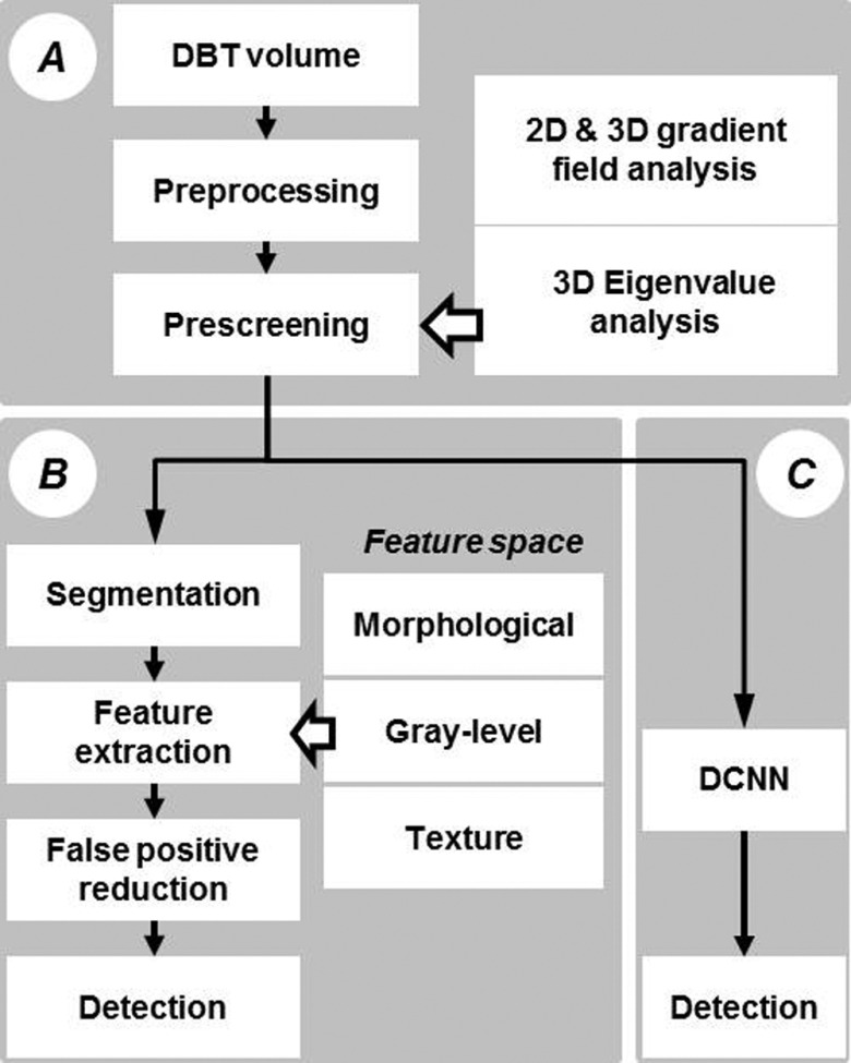
The two CAD systems for detection of masses in DBT to be compared in this study are shown in Fig. 1. Module A is common to both the feature-based CAD system and the DCNN-based CAD system. An input reconstructed DBT volume first undergoes preprocessing and prescreening of mass candidates using a combination of first-order and second-order based features. The mass candidates are then passed onto the next module for FP reduction. Module B is our previously developed feature-based FP reduction approach that extracts morphological, gray level, and texture features and combines the selected features with a classifier for discrimination of FPs. Module C is the new DCNN-based FP reduction approach that uses a trained DCNN to differentiate true masses and FPs. In the following, we will describe briefly the prescreening process and in detail the transfer training of the DCNN as well as the comparison of the performance of the DCNN-based CAD system to that of the feature-based CAD system in an independent test set.
FIG. 1.
Flow chart of CAD systems using feature and DCNN approaches. Module A: preprocessing and prescreening, which is a common module for both approaches. Module B: conventional CAD methods using feature extraction and false-positive reduction. Module C: lesion recognition and false-positive reduction using DCNN.
2.A. Data sets
SFM and DM cases were collected in the Department of Radiology at the University of Michigan Health System (UM) with Institutional Review Board (IRB) approval. Additional SFM cases were collected from the University of South Florida (USF) digitized mammogram database.34 The mammograms in the SFM-UM and SFM-USF sets were digitized using a Lumisys 200 laser scanner with an optical density (OD) range of 0–3.6 and a LUMISCAN 85 laser scanner with an OD range of 0–4.0, respectively, with 4096 gray levels. All SFMs were digitized at a pixel resolution of 50 × 50 μm and were downsampled to 100 × 100 μm by averaging every 2 × 2 neighboring pixel. DM images at UM were acquired with a GE Senographe 2000D FFDM system at a pixel size of 100 × 100 μm. The GE system uses a CsI phosphor/a:Si active matrix flat panel digital detector and the raw images were acquired at 14 bits/pixel.
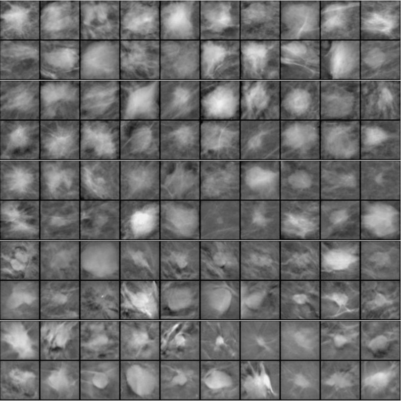
The DBT data set included cases collected at UM and cases at Massachusetts General Hospital (MGH)31,32,35 with IRB approval of the respective institutions. At UM, the DBT cases were acquired in craniocaudal (CC) and mediolateral oblique (MLO) views with a General Electric (GE) GEN2 prototype DBT system using a total tomographic angular range of 60°, 3° increments, and 21 projection views (PVs). At MGH, DBT cases were acquired in MLO view only with a prototype GE DBT system using a 50° tomographic angle, 3° increments, and 11 PVs. Both sets of DBTs (DBT-UM and DBT-MGH) were reconstructed to 1-mm slice spacing and an in-plane resolution of 100 × 100 μm using simultaneous algebraic reconstruction technique (SART),36 and the reconstructed slices were outputted at 12 bits/pixel. The DBT-UM set consisted of 186 views from 94 breasts with 179 masses, of which 61 masses were malignant and 118 masses were benign. The mass were either out of the field of view or occult in seven views, resulting in a fewer number of masses than the number of views. Two breasts had only single views. The DBT-MGH set consisted of 138 views from 138 breasts, of which 87 were malignant and 51 were benign. The details of the data sets are described in Table I. Figure 2 illustrates examples of the extracted region-of-interest (ROI) from the five data sets. All the ROIs are processed with background correction method as described in Sec. 2.D.3.
TABLE I.
Data sets used for DCNN training and testing.
| Data type | No. of views | No. of lesions | No. of TP ROIs | No. of FP ROIs | Total no. of ROIs after data augmentation |
|---|---|---|---|---|---|
| Mammography–DCNN training | |||||
| SFM-UM | 1665 | 1802 | 1802 | — | 14 416 |
| SFM-USF | 277 | 322 | 322 | — | 2 576 |
| DM | 340 | 337 | 337 | 3 173 | 28 080 |
| Total mammography training set | 2282 | 2461 | 2461 | 3 173 | 45 072 |
| DBT–DCNN training | |||||
| DBT-MGH | 138 | 138 | 690 | — | 5 520 |
| DBT-UM (training) | 92 | 90 | 450 | 28 330 | 31 930 |
| Total DBT training set | 230 | 228 | 1140 | 28 330 | 37 450 |
| DBT–CAD performance evaluation (independent test) | |||||
| DBT-UM test set | 94 | 89 | 1125 | 27 180 | 28 305 |
Note: For both TP and FP objects in DBT, 5 consecutive slices centered at the computer-detected object centroid or at the radiologist-marked best slice (for the TPs in the training set) were used for each object. For the training set, each TP ROI was augmented by rotation in 4 directions and flipping, resulting in 8 ROIs. The FP ROIs were not rotated or flipped. For the test set, all mass candidates were obtained from the prescreening step and a mass candidate might be split into multiple objects (ROIs). The entire set of available ROIs including mammography training, DBT training and DBT test sets was given by the sum of the 3 boldface values, totaling 110, 827.
FIG. 2.
Example ROIs of 128 × 128 pixels in size extracted from images with a pixel size of 200 × 200 μm. Rows 1 and 2: SFM-UM set, rows 3 and 4: from SFM-USF set, rows 5 and 6: DM, rows 7 and 8: DBT-MGH set, and rows 9 and 10: DBT-UM set. All the ROIs are background corrected.
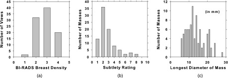
The data sets were partitioned into training and test subsets for DCNN training and CAD performance evaluation. Images from the same case were assigned to the same subset to keep the two subsets independent. The mass in each view was marked by a Mammography Quality Standards Act (MQSA) radiologist with a 2D or 3D bounding box for mammogram and DBT, respectively, as reference standard. The best slice of each mass in the DBT cases was also marked. The number of views, masses, true positive (TP) ROIs, and FP ROIs are shown in Table I. For the training of the DCNN, heterogeneous mass candidates from SFM, DM, and DBT were used. All images or slices were downsampled to 200 × 200 μm by averaging every 2 × 2 adjacent pixel; ROIs of 128 × 128 pixels containing the masses were then extracted. For DBT, ROIs were extracted from the best slice plus two slices above and two slices below. The TP class was represented by the ROIs extracted from the radiologist-marked locations. The FP class was represented by the ROIs extracted from the prescreening step of the CAD systems (see Sec. 2.B) developed for DM (Ref. 37) and DBT.33,35 The DCNN training set included 2461 lesions from 2282 SFM and DM views and 228 lesions from 230 DBT views. To augment the training patterns, each ROI was rotated and flipped to generate eight patterns. After data augmentation, total mammography training set included 19 688 TPs and 25 384 FPs ROIs. For the DBT training set, the FP ROIs were not rotated and flipped because of the large number of FPs obtained from prescreening so that it included 9120 TPs and 28 330 FPs ROIs. In total there were over 82 000 SFM, DM, and DBT ROIs for DCNN training. Testing was only performed in the DBT CAD systems. The independent test set consisted of UM cases only with a total of 94 views from 47 breasts with 89 lesions, of which 30 are malignant and 59 benign. Both TP and FP objects were detected by the prescreening module. Five slices were obtained from each detected object, resulting in a total of 28 305 ROIs, of which 1125 were considered TPs when compared with the radiologist-marked mass location. The DCNN trained with transfer learning was evaluated by an independent test set of DBT cases. The distributions of breast density, subtlety rating, and the longest diameter of the masses in the test set are shown in Fig. 3.
FIG. 3.
Histograms of (a) BI-RADS breast density categories, (b) subtlety rating, and (c) the longest diameter of the masses in the DBT test set (median = 12.5 mm, range: 5.5–28.4 mm). A subtlety rating of 1 refers to the most conspicuous lesion.
2.B. Prescreening
The prescreening stage of the CAD system identifies mass candidates in the reconstructed DBT volume (Module A in Fig. 1). This module is common to both the feature-based CAD and DCNN-based CAD systems. For this step, the DBT slices are further downsampled to a pixel size of 400 × 400 μm by averaging every adjacent 2 × 2 pixel. The downsampled DBT volume is preprocessed using a 3D Laplacian operator, and the breast region is detected using a breast boundary detection algorithm.38,39 The potential mass candidates are detected and ranked using first-order and second-order based features as follows. At every pixel location, the gradient field is calculated over a circular region of 12 mm (30 pixels) in radius centered at the pixel. Within the circle, three concentric annular rings are defined and the gradient vector at each pixel is computed and projected along the radial unit vector from the pixel to the center pixel. The average radial gradient within each ring is estimated over the pixels in the ring. The maximum of the average radial gradients among the three rings is used as a first-order gradient field feature at the center pixel. The first-order gradient field feature is calculated for all pixels on the image and normalized to a range between 0 and 1 to form a 2D gradient field convergence map. Similarly, a 3D gradient field convergence map at every voxel is obtained by performing the above procedures in 3D spherical shells in the breast volume. The maximum within a local neighborhood of voxels having gradient field convergence values above a threshold of 0.3 in the 3D gradient field convergence map is identified as a potential mass candidate location. For each identified candidate location, a 12 × 12 × 5 mm box centered at that voxel is defined. The Hessian matrix (H) containing partial second-order derivatives is calculated and the eigenvalues of H, λ1, λ2, and λ3 (λ1 < λ2 < λ3), are derived at each voxel in the box. Two mean eigenvalue features, μλi (i = 1, 2), for the mass candidate are obtained by averaging the corresponding eigenvalues over the voxels in the box. A linear discriminant classifier is used to combine the 2D and 3D gradient field convergence features and the two eigenvalue features to generate a candidate-likelihood score. By combining the first- and second-order features of the mass candidates, the TP objects would acquire higher ranking in the list of candidate objects and therefore increase the chance of the true masses being kept as mass candidates without retaining a large number of FPs.40 The top N highest candidate-likelihood score locations are identified as mass candidates and pass onto the feature-based or the DCNN-based FP reduction module.
2.C. Feature-based CAD
In our feature-based CAD system,31,33 the mass candidates identified at prescreening will undergo segmentation and feature extraction in the DBT volume with a pixel size of 200 × 200 μm in the in-plane direction. At each mass candidate location, a volume-of-interest (VOI) with a fixed in-plane size of 51.2 × 51.2 mm and an adaptive size along the depth direction is centered at that location.33 The adaptive size in the depth direction is estimated from the object size obtained by an initial 3D clustering. Three-dimensional active contour segmentation is then performed within the VOI using the initial object from 3D clustering for initialization.
In the feature extraction step, three types of features are extracted from the segmented object: (a) morphological, (b) gray level, and (c) texture features. Morphological features include the volume of the segmented object, volume change as a result of 3D morphological opening, surface area, maximum perimeter, longest diameter, and compactness. Gray level features include the gray level statistics, contrast, and histogram features. Texture features are extracted using run-length statistics on the rubber-band straightening transformed41 2D image of the object margin. A detailed description of the features can be found elsewhere.31 A stepwise linear discriminant analysis (LDA) method for feature selection based on F-statistics is used to select the best features and weights42,43 within each type of features, resulting in three LDA classifiers. FP reduction is performed sequentially in three steps, using thresholds based on LDA discriminant scores from the morphological, gray level, and texture features in this order.
2.D. DCNN-based CAD
2.D.1. DCNN architecture and hyperparameters
DCNNs are a type of artificial neural networks composed of convolutional layers and fully connected layers within a deep architecture. During training, a DCNN learns patterns through the kernels in each convolution layer. The feature maps in one layer are generated by convolving the kernels with the feature maps in the previous layer and combining them with weights. Each feature map is connected to an activation function. The generality and the levels of abstraction of the learned patterns can vary across the layers between the input and output layers, depending on the design of the local connectivity and shared weights. To achieve rotation and translation invariance to the input patterns, the feature map is subsampled through max-pooling.44 This is critical because during prescreening of mass candidates, the mass is not always centered. For the DCNN used in this study, max-pooling is performed by taking the maximum of a patch of 3 × 3 pixels centered at each pixel in the feature map with a distance (stride) of 2 pixels to the neighboring pixels. Max-pooling selects the most responsive invariant features to represent mass margins and spiculations that are important for mass detection. All the convolution layers use rectified linear units (ReLUs) as activation function given by . Normalization within a local neighborhood of 3 × 3 regions along with ReLU results in boosting of high frequency patterns such as mass spiculations while dampening of homogeneous background regions.
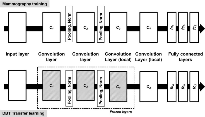
There are many possible architectural combinations for DCNN and the selection of which for a given task depends on the type and size of the input data. For the mass detection task, we have designed a DCNN architecture inspired by the work of Krizhevsky et al.45 on ImageNet46 as well as our previous work on segmentation of bladder in CT urography24,47–51 and detection of microcalcifications in DBT.52 The network in Fig. 4 has four convolution layers (C1, C2, C3, and C4) with two sets of pooling and normalization layers between C1 and C2, and C2 and C3. The four convolutional layers have 32, 32, 32, and 16 filter kernels of sizes 11 × 11, 7 × 7, 5 × 5, and 5 × 5, respectively. The three fully connected layers, fca, fcb, and fc2 contain 1024, 100, and 2 neurons, respectively. A softmax regression layer is used to calculate the cross-entropy loss during the training phase. All the weights are initialized randomly by sampling from Gaussian distribution. A learning rate of 0.002 was experimentally chosen and used for all the layers. The cuda-convnet developed by Krizhevsky et al.45 was used for designing the DCNN architecture and training.
FIG. 4.
The deep CNN architecture designed for this study. The DCNN is composed of four convolutional layers, pooling, normalization layers, and three fully connected layers. The input is 13 225 dimensional and the number of neurons in the consecutive convolutional layers is 380 192, 86 528, 18 432, and 7744. The fully connected layers have 1024, 100, and 2 neurons for fca, fcb, and fc2, respectively. The architecture shown on the top is used during training with mammography data. The architecture at the bottom is used during transfer learning with DBT data, for which the layers C1, C2, and C3 are frozen with learning rate set to 0.
The DCNN is first trained on the mammographic ROIs to differentiate the TP and FP classes. True lesions are labeled as 1 and FPs are labeled as 0 in the training set. The DBT training set is used as a validation set to monitor over-fitting. The area under the receiver operating characteristic (ROC) curve (AUC) is used as a performance metric for the classification task during the training process. After pretraining with mammogram ROIs, the weights in the layers C1, C2, and C3 are frozen with learning rate set to 0. The weights in the C4 and the fully connected layers are randomly initialized again. The DBT ROIs from the training set are then used to continue training of the DCNN.
2.D.2. Regularization of DCNN
Regularization of DCNN during training is achieved through jittering in the input layer and dropout of nodes (or neurons) in all hidden layers. For the input layer, the probability of jittering is set at 0.2, i.e., from the input ROI size of 128 × 128, a 115 × 115 ROI is randomly cropped for training. The ROI is also flipped vertically with a probability of 0.5. Dropout is a method of randomly dropping a node in a hidden layer and all the input and output connections of this node during training of each input training sample. The dropout probability for all the hidden nodes is set at 0.5. The method has been proven to reduce overfitting by preventing co-adaptation of nodes.53 In addition to the jittering and dropout techniques, the network when training on mammography data is monitored for overfitting through validation on the DBT training set.
2.D.3. Background correction
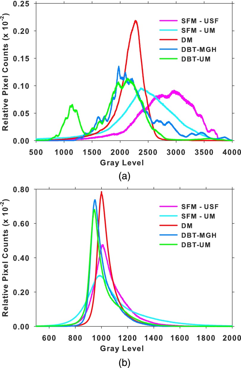
Data normalization is an important and data-dependent process for DCNN training. In our application, we normalized the data as follows. The DM images were accessed in raw format to avoid dependence on manufacturer’s processing method. The raw DM images were subjected to a simple inverted logarithmic transformation54 before background correction. The DM and DBT images were downsampled to a 200 × 200 μm image by averaging every 2 × 2 adjacent pixel. The digitized SFM-UM and SFM-USF images were downsampled to a 200 × 200 μm image by averaging every 4 × 4 adjacent pixel from the original 50 × 50 μm pixels size. An ROI of 128 × 128 pixels centered at the object of interest (mass or FPs) was then extracted from the downsampled image. The five types of heterogeneous data (SFM-UM, SFM-USF, DM, DBT-UM, and DBT-MGH) have different grayscale distributions. To reduce this variability, all the ROIs are subjected to background correction.16,55 This process also has the advantage of correcting the variations in the background gray levels that depend mainly on the overlapping breast tissue and the x-ray exposure conditions. Initially, a background image is calculated from the ROI,
where B(i, j) is the calculated gray value at pixel (i, j) of the background image, L, R, U, and D are the average gray values inside four boxes of size 8 × 8 pixels at the left, right, upper, and bottom periphery of the ROI, weighted inversely by the perpendicular distance of dl, dr, du, and dd from the pixel (i, j) to the respective boundary of the ROI. The background image is then subtracted from the ROI to obtain the background-corrected ROI. Figure 5 shows the gray level histograms of all the pixels in the ROIs from the five data sets before and after background correction.
FIG. 5.
Histograms of the gray levels of all ROIs within each type of data. The area under the histogram is normalized to 1 for all histograms. (a) Before background correction and (b) after background correction.
2.D.4. Mass detection
The trained DCNN is incorporated into the DCNN-based CAD system for FP reduction (Module C in Fig. 1). At the prescreening step of the CAD system, the top 100 objects with the highest likelihood scores are kept as mass candidates. For each prescreened and ranked mass candidate location, a 128 × 128 pixels ROI at a pixel size of 200 × 200 μm is extracted from five DBT slices centered at the object centroid. The ROI from each slice is background corrected and input into the DCNN network to obtain a score. The maximum of the five scores from the five slices is assigned as the object score. These objects may result in lesion candidates that overlap with one another. As a final step, all objects are checked for overlap and the objects are merged into one if the centroid of the bounding box of one object overlaps with another. The maximum of the individual object scores is retained as the lesion-likelihood score of the merged object.
2.E. Performance analysis
2.E.1. Free-response ROC (FROC) analysis
The final set of retained objects after merging is compared to the reference mass location marked by the experienced radiologist. If the centroid of a detected object is inside the radiologist-marked box or vice versa, the object is marked as a TP. A FROC curve is used to assess the performance of mass detection and localization. For the DCNN-based CAD, the DCNN lesion likelihood score is used as a decision variable to generate the FROC curve. For the feature-based CAD, the LDA score from the texture features is used as the decision variable to generate the FROC curve. Two sets of FROC curves are generated: (a) lesion-based, where the same lesion imaged in the CC and MLO view is considered to be a different target for detection, and (b) breast-based, where the same lesion imaged in the two views of the breast is considered to be a single target and detection of one or both is considered a TP.
2.E.2. Non-parametric method for FROC comparison
The non-parametric method compares the performance of two CAD systems using the difference in the areas under the FROC curves as a performance metric.56,57 The method uses bootstrap test to resample ranks of the CAD output scores while making no parametric assumptions. For each sample, the “bootstrapped” difference performance metric is calculated. The distribution of the bootstrap difference metric is then compared to the difference in the observed metric . If the width of the calculated distribution is much smaller than the observed metric, then the difference between the methods is concluded as significant. The fraction of the bootstrap metrics less than zero is the type I reject probability p. The method inherently accounts for the correlation of CAD scores within a patient case and also for unequal number of CAD marks between two methods within a patient case. The statistical significance of the performance difference between the feature-based and DCNN-based CAD systems is estimated from the breast-based FROC curves.
3. RESULTS
3.A. DCNN training on mammography data
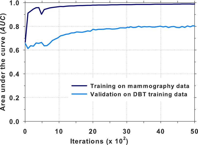
The DCNN architecture shown in Fig. 4 was trained using about 45 000 ROIs (44% TPs and 56% FPs) from the mammography data sets (Table I). The network was trained for 5000 iterations; at a given iteration, the input ROIs were randomly divided into minibatches of 256 samples. The ROI-based AUC was estimated for each iteration during the DCNN training process. The DBT ROIs from the training set were used for validation as shown in Fig. 6. A training AUC of 0.99 was achieved at a validation AUC of 0.81. It is seen that the AUC was relatively stable between 3000 and 5000 iterations. The AUC at iteration 4070 was about the average and near the mid point of this region. The weights at iteration 4070 were chosen for transfer learning. The training of the DCNN was performed on an NVIDIA Tesla K20 GPU with an execution time of approximately 8 days, which included the output of the DCNN status and the calculation of the AUC for monitoring of the training process.
FIG. 6.
Training of DCNN on mammography data and validation on the DBT training data. The iteration at 4070 with a training AUC of 0.99 and a validation AUC of 0.81 was selected for transfer learning.
3.B. Transfer learning from mammography to DBT
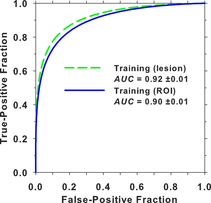
The DBT training set included five ROIs from each mass from the MGH and UM data sets and FPs from the DBT-UM set. A total of about 37 000 ROIs (26% TPs and 74% FPs) were used for training (Table I). At a given iteration, the DBT training ROIs were again randomly divided into minibatches of 256 samples, similar to the pretraining with mammographic data. Since only a convolution layer and the fully connected layers needed to be trained after freezing the rest of the architecture and it was observed by other investigators that fine-tuning of pretrained DCNN models is typically robust when dropout-backpropagation is used,58 no additional validation set was used for monitoring at this training stage. Figure 7 shows the ROC curves and AUCs of the DBT training set after transfer learning for about 1800 iterations. The ROI-based performance was obtained by treating each ROI as a sample while the lesion-based performance was obtained by taking the maximum DLNN score of the five ROIs from each object as a sample for the ROC analysis.
FIG. 7.
ROI-based and lesion-based ROC curves and their AUCs for the DBT training set after DCNN transfer learning.
3.C. Performance evaluation
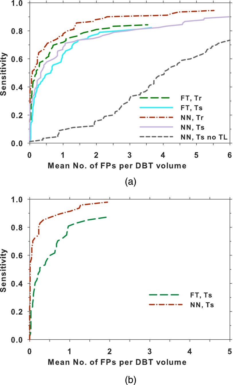
Figure 8(a) compares the lesion-based FROC curves after the prescreening objects from the training set and the test set were assessed by the feature-based and the DCNN-based FP reduction modules (Fig. 1). For the DBT training set, the feature-based CAD attained a maximum sensitivity of 85% at 3.6 FPs/view and the DCNN-based CAD attained 94% at 5.5 FPs/view. For the DBT test set, 99% of the mass objects were detected at the prescreening stage with 60 FPs/volume. The feature-based CAD attained a maximum sensitivity of 82% at 3.6 FPs/view and the DCNN-based CAD attained a maximum sensitivity of 90% at 6.0 FPs/view. For comparison, the performance of the DCNN trained with only the mammogram ROIs without transfer learning is also shown; its FROC curve on the test set was substantially lower than the other two test curves. The breast-based FROC curves are compared in Fig. 8(b). Only the results for the DBT test set are shown. Table II lists the mean number of FPs per DBT volume at several lesion-based and breast-based sensitivities for the two CAD systems.
FIG. 8.
Comparison of the FROC curves for the feature-based CAD and DCNN-based CAD systems on the DBT training and test sets. (a) Lesion-based FROC curves: a lesion in each view was counted as an independent target. The test FROC curve using the DCNN without transfer training is also shown. (b) Breast-based FROC curves: each lesion in a breast was considered to be TP if it was detected in either one or both views. The FP rate per volume (or view) was plotted. FT: feature-based, NN: DCNN-based, Tr: training, Ts: testing, TL: transfer learning.
TABLE II.
Mean number of FPs per DBT volume at several sensitivities from the FROC curves of the DBT training and test sets.
| Feature-based | DCNN-based | |||
|---|---|---|---|---|
| Mean number of FPs per DBT volume | Mean number of FPs per DBT volume | |||
| Sensitivity (%) | Lesion-based | Breast-based | Lesion-based | Breast-based |
| Training | ||||
| 60 | 0.50 | — | 0.23 | — |
| 70 | 0.85 | — | 0.50 | — |
| 80 | 2.00 | — | 1.14 | — |
| 85 | 3.60 | — | 1.40 | — |
| Test | ||||
| 60 | 0.96 | 0.49 | 0.71 | 0.05 |
| 70 | 1.29 | 0.70 | 1.06 | 0.07 |
| 80 | 2.70 | 0.97 | 2.94 | 0.29 |
| 85 | — | 1.44 | 4.60 | 0.34 |
| 90 | — | — | — | 0.82 |
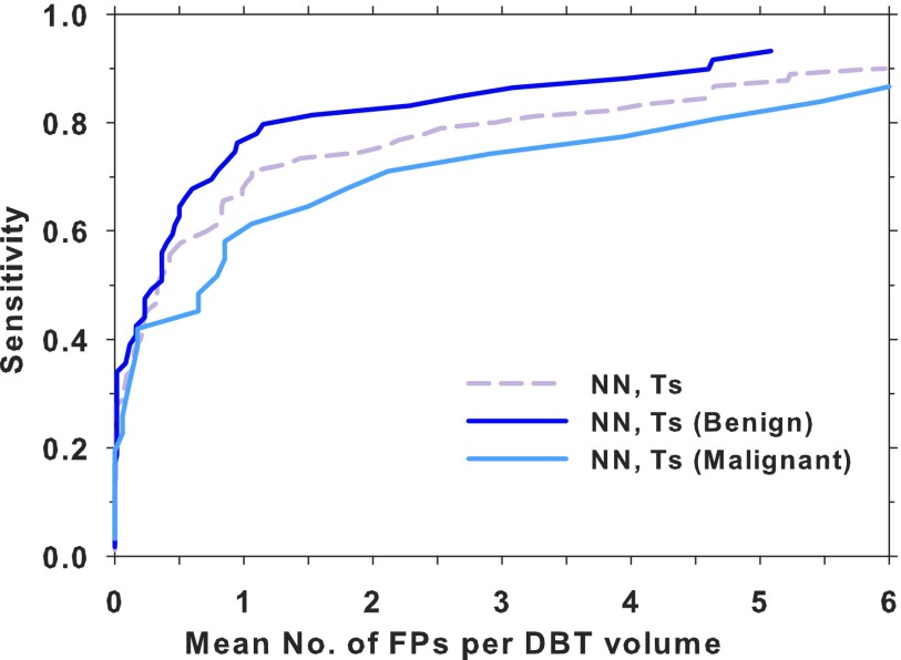
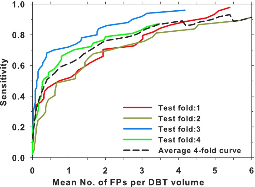
Figure 9 shows a comparison of the lesion-based test FROC curves using the DCNN-based FP reduction module for the subsets of malignant and benign masses and the entire test set. A fourfold cross validation was also performed by combining the DBT-UM and DBT-MGH cases, which were then split into four subsets with the constraints that the proportion of malignant and benign cases, as well as the ratio of UM and MGH cases, were kept approximately equal in the four subsets. In each fold, three subsets were used for transfer training of the same DCNN pretrained with mammography ROIs and one subset for testing. A test FROC curve using only the DBT-UM cases in the subset was generated as the properties of the test samples would be closer to those of the test FROC curve in Fig. 8(a). Figure 10 shows the four test FROC curves together with an average test FROC curve from the curves of the subsets.
FIG. 9.
Comparison of the lesion-based FROC curves for the DCNN-based CAD system on the entire DBT test set and the malignant (30 masses in 34 views) and benign (59 masses in 60 views) DBT test subsets. NN: DCNN-based, Ts: testing.
FIG. 10.
Comparison of the lesion-based FROC curves for the DBT-UM cases in the test subsets obtained by using the DCNN trained and tested by fourfold cross validation. An average curve of the four curves is also shown.
Using the non-parametric method, the difference in the areas under the FROC curves at a threshold of 2 FPs/view [i.e., the figures-of-merit (FOM)] between the breast-based FROC curves for the two methods is statistically significant (p value = 0.027), as shown in Table III.
TABLE III.
Comparison of the breast-based FROC curves for the DBT test set between the feature-based CAD and the DCNN-based CAD by the non-parametric method. The FOM is the difference in the area under the FROC curve between the two methods at a threshold of 2 FPs/view; CI: 95% confidence interval.
| CAD | FOM | CI | p value |
|---|---|---|---|
| Previous feature-based CAD | 0.325 | (0.0334, 0.6055) | 0.027* |
| Current DCNN-based CAD |
4. DISCUSSION
We trained a DCNN for mass detection using a deep architecture with four convolutional layers and three fully connected layers (Fig. 4). The DCNN was trained first using mammography data from SFM and DM modalities and subsequently underwent transfer learning with masses in DBT. Both the mammography and DBT training stages had the same output classes, true masses, and FPs. The heterogeneous data used for DCNN training were matched to a consistent gray level range. As shown in Fig. 5, the different gray level distributions of the ROIs were adjusted to a common reference range by background correction. The background correction also has the advantage of reducing the non-uniformity of the ROIs due to variations in the low-frequency gray levels from overlapping breast tissue and x-ray exposure.16,55 To assess the effect of background correction, we trained a smaller DCNN with four convolution layers and a fully connected output layer,59 where the first two convolution layers were connected by max-pooling and normalization layers. We followed the trends of the training and validation AUCs as the number of iterations increased at several learning rates. The results using this smaller DCNN indicated that normalization of the data, i.e., background correction for the ROIs in this study, could improve the stability of training and the trained DCNN could generalize better in terms of AUC. Because of the hyperparameter space and the numerous possible combinations of parameters for both the with- and without-background correction conditions, we did not attempt to investigate the effect of background correction on performance (AUC) again with the large DCNN shown in Fig. 4.
Training of neural networks usually requires a validation set to monitor overfitting, and even more so with DCNN that is a very large network with hundreds of thousands of parameters. When the DCNN performance for the validation set reaches a stable plateau, training should be terminated or overfitting to the training samples may occur. Some interesting results can be observed from the training of DCNN with mammography data in Fig. 6, which shows that, at a training AUC of 0.99, the DCNN reached a validation AUC of 0.81 on the DBT training set. In other words, the average sensitivity of detecting a randomly chosen DBT mass was about 80% when a DCNN is trained only with mammography data. This indicates that there is a substantial degree of similarity in the low-level features, as recognized by the DCNN, between masses in mammography and DBT. However, DBT has some unique patterns that are different from those on SFM and DM. The reduced overlapping of the fibroglandular tissue in DBT results in clearer mass margins than those in mammography and more homogeneous background. These detailed features are learned by training the last (C4) convolution layer as well as the three fully connected layers with DBT masses during transfer learning. Moreover, due to the nature of limited-angle tomography, DBT suffers from intraslice and interslice artifacts. These artifacts in DBT contribute to differences in the appearance of masses from those in mammography. This preliminary study shows that the transfer learned DCNN after training with the DBT data set achieved an ROI-based and lesion-based AUC of 0.90 and 0.92, respectively (Fig. 7), which was a substantial improvement from the AUC of 0.81 before the additional training with DBT. Further studies are needed to assess the differences between mass features in mammography and DBT and to investigate if the knowledge from one modality can be learned and transferred to another modality more efficiently and effectively by the DCNN.
In the CAD systems, the potential mass candidates are detected through a combination of first- and second-order features at the prescreening stage. The top N candidates from the ranked list based on the candidate likelihood score are passed to the DCNN. Figure 8 shows that the lesion-based test FROC curves for the two methods are comparable in differentiation of individual masses from FPs but the DCNN-based method can differentiate TPs and FPs more accurately than the feature-based method in breast-based detection performance. The non-parametric method in Table III shows that the difference in the breast-based FROC curves between the two methods is statistically significant. The DCNN-based method does not require the segmentation and feature extraction steps compared to the feature-based method; it is therefore less dependent on the specific methods and parameters designed for these steps. Nevertheless, the DCNN-based method depends on the availability of a large and diverse set of training samples as well as on the architecture and regularization method of the DCNN to learn the complex patterns of masses. The DCNN-based method might be less influenced by lesion-specific features than the feature-based method, resulting in a better chance of recognizing a mass in at least one of the views and a significantly better breast-based detection performance. We will continue to collect a larger DBT data set for training and testing the systems and further investigate the learning and generalizabilities of the two methods.
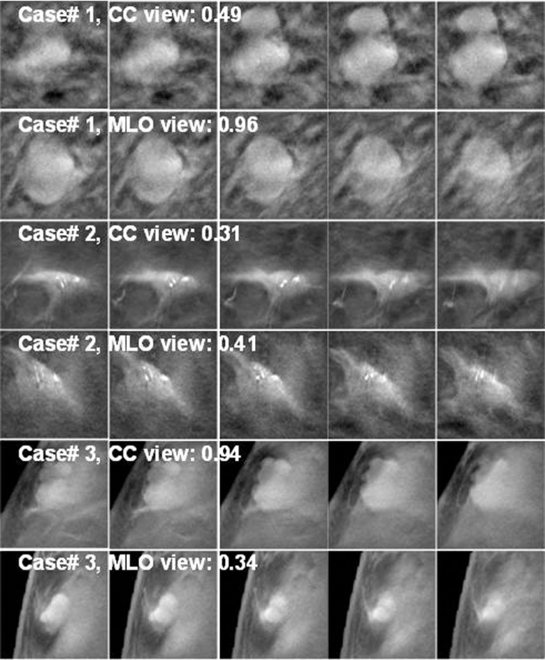
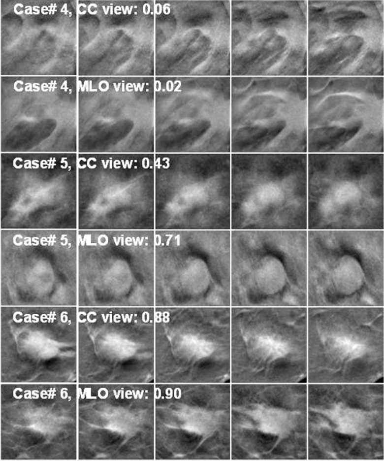
Figure 11 shows examples of mass ROIs in the training set, for which the DCNN failed to correctly train in one or both views. In case#1, two lesions appeared within the 128 × 128 pixels ROIs. The lesions were seen clearly in the CC view, but overlapped in the MLO view. The CC-view mass had lower score and the MLO-view mass had a score closer to 1. Case#2 had microcalcifications on a mass and both views scored very low, probably because there were very few mass examples with microcalcifications in the training set and the DCNN did not learn the pattern well. In case#3, the mass appeared larger in CC view, which might yield the higher score than the smaller mass in MLO view. The recognition of small mass near the breast boundary may be improved if more training samples with similar features can be included in the training set. Figure 12 shows examples of mass ROIs from the test set. In case#4, even though the mass was highly spiculated, only half of the mass was imaged in the field of view and the DCNN could not recognize the pattern, resulting in very low scores. In case#5, the candidate location of the object in the CC view detected at the prescreening step was a few slices off the mass center so that the best slice of the object was missed and the scores in all five slices were relatively low. The object in the MLO view was correctly detected resulting in a relatively higher DCNN score. Case#6 is a good example that the DCNN correctly identified the mass with a high score in both views.
FIG. 11.
Examples of TPs from the DBT training set. The DCNN was trained to give a score of 1 for TPs and a score of 0 for FPs. Each ROI is 128 × 128 pixels, extracted from DBT slice of 200 × 200 μm pixels size. Each lesion was extracted as five slices centered at the prescreening object centroid location. The lesion likelihood score shown was the maximum of the five DCNN scores. In case#1, two lesions were connected and appeared clearly in CC view and had a low score, but appeared as a single overlapped lesion in the MLO view and obtained a high score.
FIG. 12.
Examples of TPs from the DBT test set. Case#4 and case#6 were biopsy-proven to be invasive ductal carcinoma and case#5 was fibrocystic disease. The lesion likelihood score shown was the maximum of the DCNN scores from the five slices. In case#4, the lesion was close to the chest wall and only part of the spiculated mass was seen on the right side of the ROIs; the DCNN failed to recognize the mass and gave very low scores for both views.
Fotin et al.60 reported 89% sensitivity at 3.25 FPs/volume for 344 DBT volumes with suspicious and malignant lesions. For 123 patients with malignant lesions from three centers, Morra et al.,61 showed a performance of 89% sensitivity at 2.7 ± 1.8 FP/volume. Schie et al.62 used a data set of 192 patients with 49 patients having at least one malignant mass to develop CAD method for malignant masses, resulting in 79% sensitivity at 3 FPs/volume. These studies reported the lesion-based detection performance for malignant masses. In comparison, our study obtained 80% sensitivity at 2.94 FPs/volume for 94 DBT volumes with 89 lesions (30 malignant and 59 benign).
There are limitations in this study. The DBT test set is not large enough to reliably analyze the performance difference between malignant and benign masses. Note that the FROC curves in Fig. 9 may not be generalizable to the population due to the small number of malignant cases and the CADe system was trained using both malignant and benign masses. The DBT was acquired with a prototype system, the geometry of which is different from clinical systems. The effect of the number of projection views and tomographic angular range on the performance of the CAD systems for masses has yet to be investigated in detail.63–65 This study shows that a convolution-based deep learning technique can be used to detect masses equally well or better than a feature-based method. With accumulation of a larger set of DBT data, we plan to conduct a detailed study to understand the extent to which mammography data can help a DCNN learn representative mass patterns observed in DBT. The effect of DCNN training with and without transfer learning will be studied. Furthermore, DCNN-based and feature-based methods might have different strengths and weaknesses. We will explore the potential of developing a CAD system that utilizes the complementary information from both methods to further improve mass detection in DBT.
5. CONCLUSION
Unlike previous studies in which natural scene images were used for transfer learning to identify specific patterns in medical images, in this work we demonstrated that mammography images can be useful for pretraining of a DCNN for mass detection in DBT. The similarity between masses in mammography and DBT can be observed from the ability of the DCNN in recognizing masses in DBT with an AUC of over 80% when trained solely on masses from mammograms. We also showed that the DCNN-based CAD system outperformed the feature-based CAD system for breast-based performance and the difference was statistically significant. The DCNN-based FP reduction has the potential to replace or substantially augment the segmentation and feature extraction steps in the CAD system.
ACKNOWLEDGMENTS
This work is supported by National Institutes of Health Award No. RO1 CA151443. The authors would like to thank Frank W. Samuelson and Nicholas Petrick for providing the code and assistance with the non-parametric analysis method.
CONFLICT OF INTEREST DISCLOSURE
Mark A. Helvie, M.D., discloses an institutional grant from GE Healthcare (an activity not associated with this work).
REFERENCES
- 1.Russakovsky O., Deng J., Su H., Krause J., Satheesh S., Ma S., Huang Z., Karpathy A., Khosla A., and Bernstein M., “ImageNet large scale visual recognition challenge,” Int. J. Comput. Vision , 211–252 (2015). 10.1007/s11263-015-0816-y [DOI] [Google Scholar]
- 2.Yosinski J., Clune J., Bengio Y., and Lipson H., “How transferable are features in deep neural networks?,” in Advances in Neural Information Processing Systems (Red Hook, NY, 2014), pp. 3320–3328. [Google Scholar]
- 3.See breastscreening.cancer.gov for NCI-funded breast Cancer Surveillance Consortium (HHSN261201100031C), downloaded from the Breast Cancer Surveillance Consortium, 23 September 2013.
- 4.Broeders M., Moss S., Nyström L., Njor S., Jonsson H., Paap E., Massat N., Duffy S., Lynge E., and Paci E., “The impact of mammographic screening on breast cancer mortality in Europe: A review of observational studies,” J. Med. Screening , 14–25 (2012). 10.1258/jms.2012.012078 [DOI] [PubMed] [Google Scholar]
- 5.Lauby-Secretan B., Scoccianti C., Loomis D., Benbrahim-Tallaa L., Bouvard V., Bianchini F., and Straif K., “Breast-cancer screening—Viewpoint of the IARC Working Group,” N. Engl. J. Med. , 2353–2358 (2015). 10.1056/NEJMsr1504363 [DOI] [PubMed] [Google Scholar]
- 6.Niklason L. T. et al. , “Digital tomosynthesis in breast imaging,” Radiology , 399–406 (1997). 10.1148/radiology.205.2.9356620 [DOI] [PubMed] [Google Scholar]
- 7.Wu T. et al. , “Tomographic mammography using a limited number of low-dose cone-beam projection images,” Med. Phys. , 365–380 (2003). 10.1118/1.1543934 [DOI] [PubMed] [Google Scholar]
- 8.Sechopoulos I., “A review of breast tomosynthesis. Part I. The image acquisition process,” Med. Phys. , 014301 (12pp.) (2013). 10.1118/1.4770279 [DOI] [PMC free article] [PubMed] [Google Scholar]
- 9.Fukunaga K. and Hayes R. R., “Effects of sample size on classifier design,” IEEE Trans. Pattern Anal. Mach. Intell. , 873–885 (1989). 10.1109/34.31448 [DOI] [Google Scholar]
- 10.Chan H.-P., Sahiner B., Wagner R. F., and Petrick N., “Classifier design for computer-aided diagnosis: Effects of finite sample size on the mean performance of classical and neural network classifiers,” Med. Phys. , 2654–2668 (1999). 10.1118/1.598805 [DOI] [PubMed] [Google Scholar]
- 11.Shin H.-C., Roth H. R., Gao M., Lu L., Xu Z., Nogues I., Yao J., Mollura D., and Summers R. M., “Deep convolutional neural networks for computer-aided detection: CNN architectures, dataset characteristics and transfer learning,” IEEE Trans. Med. Imaging , 1285–1298 (2016). 10.1109/TMI.2016.2528162 [DOI] [PMC free article] [PubMed] [Google Scholar]
- 12.Näppi J. J., Hironaka T., Regge D., and Yoshida H., “Deep transfer learning of virtual endoluminal views for the detection of polyps in CT colonography,” Proc. SPIE , 97852B-1–97852B-8 (2016). 10.1117/12.2217260 [DOI] [Google Scholar]
- 13.Cruz-Roa A., Arévalo J., Judkins A., Madabhushi A., and González F., “A method for medulloblastoma tumor differentiation based on convolutional neural networks and transfer learning,” Proc. SPIE , 968103-1–968103-8 (2015). 10.1117/12.2208825 [DOI] [Google Scholar]
- 14.Tajbakhsh N., Shin J. Y., Gurudu S. R., Hurst R. T., Kendall C. B., Gotway M. B., and Liang J., “Convolutional neural networks for medical image Analysis: Full training or fine tuning?,” IEEE Trans. Med. Imaging , 1299–1312 (2016). 10.1109/TMI.2016.2535302 [DOI] [PubMed] [Google Scholar]
- 15.Chan H.-P., Lo S. C. B., Sahiner B., Lam K. L., and Helvie M. A., “Computer-aided detection of mammographic microcalcifications: Pattern recognition with an artificial neural network,” Med. Phys. , 1555–1567 (1995). 10.1118/1.597428 [DOI] [PubMed] [Google Scholar]
- 16.Sahiner B., Chan H.-P., Petrick N., Wei D., Helvie M. A., Adler D. D., and Goodsitt M. M., “Classification of mass and normal breast tissue: A convolution neural network classifier with spatial domain and texture images,” IEEE Trans. Med. Imaging , 598–610 (1996). 10.1109/42.538937 [DOI] [PubMed] [Google Scholar]
- 17.Ge J., Sahiner B., Hadjiiski L. M., Chan H.-P., Wei J., Helvie M. A., and Zhou C., “Computer aided detection of clusters of microcalcifications on full field digital mammograms,” Med. Phys. , 2975–2988 (2006). 10.1118/1.2211710 [DOI] [PubMed] [Google Scholar]
- 18.Samala R. K., Chan H.-P., Lu Y., Hadjiiski L., Wei J., and Helvie M. A., “Digital breast tomosynthesis: Computer-aided detection of clustered microcalcifications on planar projection images,” Phys. Med. Biol. , 7457–7477 (2014). 10.1088/0031-9155/59/23/7457 [DOI] [PMC free article] [PubMed] [Google Scholar]
- 19.Samala R. K., Chan H.-P., Lu Y., Hadjiiski L. M., Wei J., and Helvie M. A., “Computer-aided detection system for clustered microcalcifications in digital breast tomosynthesis using joint information from volumetric and planar projection images,” Phys. Med. Biol. , 8457–8479 (2015). 10.1088/0031-9155/60/21/8457 [DOI] [PMC free article] [PubMed] [Google Scholar]
- 20.Lo S. C., Lou S. L., Lin J. S., Freedman M. T., and Mun S. K., “Artificial convolution neural network techniques and applications to lung nodule detection,” IEEE Trans. Med. Imaging , 711–718 (1995). 10.1109/42.476112 [DOI] [PubMed] [Google Scholar]
- 21.Lo S. C. B., Chan H.-P., Lin J. S., Li H., Freedman M., and Mun S. K., “Artificial convolution neural network for medical image pattern recognition,” Neural Networks , 1201–1214 (1995). 10.1016/0893-6080(95)00061-518263408 [DOI] [Google Scholar]
- 22.Samala R. K., Chan H.-P., Hadjiiski L., and Helvie M., “Analysis of computer-aided detection techniques and signal characteristics for clustered microcalcifications on digital mammography and digital breast tomosynthesis,” Phys. Med. Biol. , 7092–7112 (2016). 10.1088/0031-9155/61/19/7092 [DOI] [PMC free article] [PubMed] [Google Scholar]
- 23.Kooi T., Gubern-Merida A., Mordang J.-J., Mann R., Pijnappel R., Schuur K., den Heeten A., and Karssemeijer N., “A comparison between a deep convolutional neural network and radiologists for classifying regions of interest in mammography,” in Proceedings of the 13th International Workshop on Digital Mammography (Springer International Publishing, Switzerland, 2016), pp. 51–56. [Google Scholar]
- 24.Cha K. H., Hadjiiski L., Samala R. K., Chan H.-P., Caoili E. M., and Cohan R. H., “Urinary bladder segmentation in CT urography using deep-learning convolutional neural network and level sets,” Med. Phys. , 1882–1896 (2016). 10.1118/1.4944498 [DOI] [PMC free article] [PubMed] [Google Scholar]
- 25.Gao M., Bagci U., Lu L., Wu A., Buty M., Shin H.-C., Roth H., Papadakis G. Z., Depeursinge A., and Summers R. M., “Holistic classification of CT attenuation patterns for interstitial lung diseases via deep convolutional neural networks,” Comput. Methods Biomech. Biomed. Eng.: Imaging Visualization 1–6 (2016). 10.1080/21681163.2015.1124249 [DOI] [PMC free article] [PubMed] [Google Scholar]
- 26.Ciompi F., de Hoop B., van Riel S. J., Chung K., Scholten E. T., Oudkerk M., de Jong P. A., Prokop M., and van Ginneken B., “Automatic classification of pulmonary peri-fissural nodules in computed tomography using an ensemble of 2D views and a convolutional neural network out-of-the-box,” Med. Image Anal. , 195–202 (2015). 10.1016/j.media.2015.08.001 [DOI] [PubMed] [Google Scholar]
- 27.Zuley M. L., Bandos A. I., Abrams G. S., Cohen C., Hakim C. M., Sumkin J. H., Drescher J., Rockette H. E., and Gur D., “Time to diagnosis and performance levels during repeat interpretations of digital breast tomosynthesis: Preliminary observations,” Acad. Radiol. , 450–455 (2010). 10.1016/j.acra.2009.11.011 [DOI] [PubMed] [Google Scholar]
- 28.Astley S. et al. , “A comparison of image interpretation times in full field digital mammography and digital breast tomosynthesis,” Proc. SPIE , 86730S-1–86730S-8 (2013). 10.1117/12.2006039 [DOI] [Google Scholar]
- 29.Bernardi D., Ciatto S., Pellegrini M., Anesi V., Burlon S., Cauli E., Depaoli M., Larentis L., Malesani V., and Targa L., “Application of breast tomosynthesis in screening: Incremental effect on mammography acquisition and reading time,” Br. J. Radiol. , e1174–e1178 (2014). 10.1259/bjr/19385909 [DOI] [PMC free article] [PubMed] [Google Scholar]
- 30.Wallis M. G., Moa E., Zanca F., Leifland K., and Danielsson M., “Two-view and single-view tomosynthesis versus full-field digital mammography: High-resolution x-ray imaging observer study,” Radiology , 788–796 (2012). 10.1148/radiol.11103514 [DOI] [PubMed] [Google Scholar]
- 31.Chan H.-P., Wei J., Sahiner B., Rafferty E. A., Wu T., Roubidoux M. A., Moore R. H., Kopans D. B., Hadjiiski L. M., and Helvie M. A., “Computer-aided detection system for breast masses on digital tomosynthesis mammograms–preliminary experience,” Radiology , 1075–1080 (2005). 10.1148/radiol.2373041657 [DOI] [PMC free article] [PubMed] [Google Scholar]
- 32.Chan H.-P., Wei J., Zhang Y. H., Helvie M. A., Moore R. H., Sahiner B., Hadjiiski L., and Kopans D. B., “Computer-aided detection of masses in digital tomosynthesis mammography: Comparison of three approaches,” Med. Phys. , 4087–4095 (2008). 10.1118/1.2968098 [DOI] [PMC free article] [PubMed] [Google Scholar]
- 33.Wei J., Chan H.-P., Sahiner B., Hadjiiski L. M., Helvie M. A., Zhou C., and Lu Y., “Computer-aided detection of breast masses in digital breast tomosynthesis (DBT): Improvement of false positive reduction by optimization of object segmentation,” Proc. SPIE , 796311-1–796311-6 (2011). 10.1117/12.878214 [DOI] [Google Scholar]
- 34.Heath M., Bowyer K., Kopans D., Moore R., and Kegelmeyer P., “The digital database for screening mammography,” in Digital Mammography; IWDM 2000, edited byYaffe M. J. (Medical Physics Publishing, Toronto, Canada, 2001). [Google Scholar]
- 35.Chan H.-P., Wu Y. T., Sahiner B., Wei J., Helvie M. A., Zhang Y., Moore R. H., Kopans D. B., Hadjiiski L., and Way T., “Characterization of masses in digital breast tomosynthesis: Comparison of machine learning in projection views and reconstructed slices,” Med. Phys. , 3576–3586 (2010). 10.1118/1.3432570 [DOI] [PMC free article] [PubMed] [Google Scholar]
- 36.Zhang Y., Chan H.-P., Sahiner B., Wei J., Goodsitt M. M., Hadjiiski L. M., Ge J., and Zhou C., “A comparative study of limited-angle cone-beam reconstruction methods for breast tomosynthesis,” Med. Phys. , 3781–3795 (2006). 10.1118/1.2237543 [DOI] [PMC free article] [PubMed] [Google Scholar]
- 37.Wei J. et al. , “Computer aided detection systems for breast masses: Comparison of performances on full-field digital mammograms and digitized screen-film mammograms,” Acad. Radiol. , 659–669 (2007). 10.1016/j.acra.2007.02.017 [DOI] [PMC free article] [PubMed] [Google Scholar]
- 38.Zhou C., Chan H.-P., Paramagul C., Roubidoux M. A., Sahiner B., Hadjiiski L. M., and Petrick N., “Computerized nipple identification for multiple image analysis in computer-aided diagnosis,” Med. Phys. , 2871–2882 (2004). 10.1118/1.1800713 [DOI] [PMC free article] [PubMed] [Google Scholar]
- 39.Wu Y.-T., Zhou C., Hadjiiski L. M., Shi J., Wei J., Paramagul C., Sahiner B., and Chan H.-P., “A dynamic multiple thresholding method for automated breast boundary detection in digitized mammograms,” Proc. SPIE , 65122U1–65122U8 (2007). 10.1117/12.710198 [DOI] [Google Scholar]
- 40.Samala R. K., Wei J., Chan H.-P., Hadjiiski L. M., Cha K., and Helvie M. A., “First and second-order features for detection of masses in digital breast tomosynthesis,” Proc. SPIE , 978523-1–978523-7 (2016). 10.1117/12.2216327 [DOI] [Google Scholar]
- 41.Sahiner B., Chan H.-P., Petrick N., Helvie M. A., and Goodsitt M. M., “Computerized characterization of masses on mammograms: The rubber band straightening transform and texture analysis,” Med. Phys. , 516–526 (1998). 10.1118/1.598228 [DOI] [PubMed] [Google Scholar]
- 42.Way T., Sahiner B., Hadjiiski L., and Chan H.-P., “Effect of finite sample size on feature selection and classification: A simulation study,” Med. Phys. , 907–920 (2010). 10.1118/1.3284974 [DOI] [PMC free article] [PubMed] [Google Scholar]
- 43.Chan H.-P., Sahiner B., Lam K. L., Petrick N., Helvie M. A., Goodsitt M. M., and Adler D. D., “Computerized analysis of mammographic microcalcifications in morphological and texture feature space,” Med. Phys. , 2007–2019 (1998). 10.1118/1.598389 [DOI] [PubMed] [Google Scholar]
- 44.Ranzato M. A., Huang F. J., Boureau Y.-L., and Lecun Y., “Unsupervised learning of invariant feature hierarchies with applications to object recognition,” in IEEE Conference on Computer Vision and Pattern Recognition, 2007 (IEEE, 2007), pp. 1–8. 10.1109/CVPR.2007.383157 [DOI] [Google Scholar]
- 45.Krizhevsky A., Sutskever I., and Hinton G. E., “Imagenet classification with deep convolutional neural networks,” Adv. Neural Inf. Proc. Syst. 1097–1105 (2012). [Google Scholar]
- 46.Deng J., Dong W., Socher R., Li L.-J., Li K., and Fei-Fei L., “Imagenet: A large-scale hierarchical image database,” in IEEE Conference on Computer Vision and Pattern Recognition, 2009 (IEEE, 2009), pp. 248–255. 10.1109/CVPR.2009.5206848 [DOI] [Google Scholar]
- 47.Cha K. H., Hadjiiski L., Chan H.-P., Samala R. K., Cohan R. H., and Caoli E. M., “Deep-learning-based bladder segmentation in CT urography,” in RSNA Program Book, SSG16-02,2015.
- 48.Cha K. H., Hadjiiski L. M., Samala R. K., Chan H.-P., Cohan R. H., and Caoili E. M., “Comparison of bladder segmentation using deep-learning convolutional neural network with and without level sets,” Proc. SPIE , 978512-1–978512-7 (2016). 10.1117/12.2216852 [DOI] [PMC free article] [PubMed] [Google Scholar]
- 49.Cha K. H., Hadjiiski L., Chan H.-P., Samala R. K., Cohan R. H., Caoili E. M., Weizer A., and Alva A., “Deep-learning bladder cancer treatment response assessment in CT urography,” in RSNA Program Book, SSQ18-01,2016.
- 50.Cha K. H., Hadjiiski L., Samala R. K., Chan H.-P., Cohan R. H., Caoili E. M., Paramagul C., Alva A., and Weizer A., “Bladder cancer segmentation in CT for treatment response assessment: Application of deep-learning convolution neural network—A pilot study,” Tomography (2016) (accepted). [DOI] [PMC free article] [PubMed] [Google Scholar]
- 51.Cha K. H., Hadjiiski L. M., Chan H.-P., Caoili E. M., Cohan R. H., Weizer A., and Zhou C., “Computer-aided detection of bladder mass within non-contrast-enhanced region of CT Urography (CTU),” Proc. SPIE , 97853W-1–97853W-6 (2016). 10.1117/12.2216289 [DOI] [Google Scholar]
- 52.Samala R. K., Chan H.-P., Hadjiiski L. M., Cha K., and Helvie M. A., “Deep-learning convolution neural network for computer-aided detection of microcalcifications in digital breast tomosynthesis,” Proc. SPIE , 97850Y-1–97850Y-7 (2016). 10.1117/12.2217092 [DOI] [Google Scholar]
- 53.Srivastava N., Hinton G., Krizhevsky A., Sutskever I., and Salakhutdinov R., “Dropout: A simple way to prevent neural networks from overfitting,” J. Mach. Learn. Res. , 1929–1958 (2014). [Google Scholar]
- 54.Burgess A. E., “On the noise variance of a digital mammography system,” Med. Phys. , 1987–1995 (2004). 10.1118/1.1758791 [DOI] [PubMed] [Google Scholar]
- 55.Chan H.-P., Wei D., Helvie M. A., Sahiner B., Adler D. D., Goodsitt M. M., and Petrick N., “Computer-aided classification of mammographic masses and normal tissue: Linear discriminant analysis in texture feature space,” Phys. Med. Biol. , 857–876 (1995). 10.1088/0031-9155/40/5/010 [DOI] [PubMed] [Google Scholar]
- 56.Samuelson F. W., Petrick N., and Paquerault S., “Advantages and examples of resampling for CAD evaluation,” in 4th IEEE International Symposium on Biomedical Imaging: From Nano to Macro, 2007 (IEEE, 2007), pp. 492–495. [Google Scholar]
- 57.Samuelson F. W. and Petrick N., “Comparing image detection algorithms using resampling,” in 3rd IEEE International Symposium on Biomedical Imaging: Nano to Macro, 2006 (IEEE, 2006), pp. 1312–1315. [Google Scholar]
- 58.Hinton G. E., Srivastava N., Krizhevsky A., Sutskever I., and Salakhutdinov R. R., “Improving neural networks by preventing co-adaptation of feature detectors,” preprint arXiv:1207.0580 (2012).
- 59.Samala R. K., Chan H.-P., Hadjiyski L., Wei J., Cha K., and Helvie M., “Comparison of mass detection for digital breast tomosynthesis (DBT) with and without transfer learning of deep-learning convolution neural network (DLCNN) from digitized screen-film mammography (SFM) and digital mammography (DM),” in RSNA Program Book, PH256-SD-WEB5,2016.
- 60.Fotin S. V., Yin Y., Haldankar H., Hoffmeister J. W., and Periaswamy S., “Detection of soft tissue densities from digital breast tomosynthesis: Comparison of conventional and deep learning approaches,” Proc. SPIE , 97850X–97850X-6 (2016). 10.1117/12.2217045 [DOI] [Google Scholar]
- 61.Morra L., Sacchetto D., Durando M., Agliozzo S., Carbonaro L. A., Delsanto S., Pesce B., Persano D., Mariscotti G., and Marra V., “Breast cancer: Computer-aided detection with digital breast tomosynthesis,” Radiology , 56–63 (2015). 10.1148/radiol.2015141959 [DOI] [PubMed] [Google Scholar]
- 62.van Schie G., Wallis M. G., Leifland K., Danielsson M., and Karssemeijer N., “Mass detection in reconstructed digital breast tomosynthesis volumes with a computer-aided detection system trained on 2D mammograms,” Med. Phys. , 041902 (11pp.) (2013). 10.1118/1.4791643 [DOI] [PubMed] [Google Scholar]
- 63.Chan H.-P., Wei J., Zhang Y., Helvie M. A., Hadjiiski L. M., and Sahiner B., “Digital breast tomosynthesis (DBT) mammography: Effect of number of projection views on computerized mass detection using 2D and 3D approaches,” in RSNA Program Book, 2008 (RSNA, Oak Brook, IL, 2008), p. 560. [Google Scholar]
- 64.Samala R. K., Chan H.-P., Lu Y., Hadjiiski L., Wei J., and Helvie M., “Digital breast tomosynthesis: Effects of projection-view distribution on computer-aided detection of microcalcification clusters,” Proc. SPIE , 90350Y (2014). 10.1117/12.2043513 [DOI] [Google Scholar]
- 65.Chan H.-P., Wei J., Zhang Y. H., Sahiner B., Hadjiiski L., and Helvie M. A., “Detection of masses in digital breast tomosynthesis mammography: Effects of the number of projection views and dose,” in Proceedings of the 9th International Workshop on Digital Mammography IWDM-2008 (Springer, Berlin Heidelberg, 2008), pp. 279–285. [Google Scholar]


