Statistical methods for detecting differentially methylated regions based on MethylCap-seq data

Abstract

DNA methylation is a well-established epigenetic mark, whose pattern throughout the genome, especially in the promoter or CpG islands, may be modified in a cell at a disease stage. Recently developed probabilistic approaches allow distributing methylation signals at nucleotide resolution from MethylCap-seq data. Standard statistical methods for detecting differential methylation suffer from ‘curse of dimensionality’ and sparsity in signals, resulting in high false-positive rates. Strong correlation of signals between CG sites also yields spurious results. In this article, we review applicability of high-dimensional mean vector tests for detection of differentially methylated regions (DMRs) and compare and contrast such tests with other methods for detecting DMRs. Comprehensive simulation studies are conducted to highlight the performance of these tests under different settings. Based on our observation, we make recommendations on the optimal test to use. We illustrate the superiority of mean vector tests in detecting cancer-related canonical gene pathways, which are significantly enriched for acute myeloid leukemia and ovarian cancer.

Introduction

DNA methylation is an epigenetic modification known to regulate transcription and transcript splicing, and to play a role in a number of other cellular mechanisms. The dysregulation of methylation has been implicated in a variety of human diseases and cancer and is therefore extensively investigated. Whole genome bisulfite sequencing (WGBS) [1, 2] is a standard method to detect methylation status of the genome at individual nucleotide resolution. However, owing to high experimental cost, other high-throughput techniques such as reduced read bisulfite sequencing [3] and capture-based methods [4, 5] have been developed for large-scale studies. In particular, capture-based methylation assays such as MethylCap-seq are more resource-friendly for large-scale clinical trials, as these approaches require less patient material, a fraction of the sequencing depth and the associated data analysis efforts in comparison with single-base resolution WGBS. Capture-based assays do have the drawback of data resolution, as methylation signals are associated with library fragment sizes [6]. Recently, we derived a novel approach (PrEMeR-CG) [5] to compute nucleotide-resolution methylation values from MethylCap-seq data. This prompts the need to generate more sensitive statistical models by which differences between sample groups can be assayed.

To identify differentially methylated regions (DMRs) in the genome between two groups, say control and treatment, a preliminary step is to define such regions. One way is to consider well-annotated regions such as CpG islands or promoter regions. Another way is to consider the entire genome, dividing them into regions of fixed width, such as 1 kb. In such regions, methylation signal between neighboring CG sites are potentially positively correlated [7, 8]. As such, while the average or total methylation signal can be used to construct univariate testing procedures, ignorance of the dependence structure can lead to spurious results. That is, representing the methylation signal of a region by a single value such as the average or total over all sites within the region is therefore incorrect. Also there is the risk of flattening out hyper- and hypo-methylated regions, leading to reduction in power. Multivariate statistical methods that incorporate the correlation structure for detection of differential methylation within a region are alternatives that have not been extensively considered.

One of the approaches to obtain methylation coverage from MethylCap-seq reads is MEDIPS [4, 9], where the relative methylation signal or reads per kilobase per million reads value is calculated for bins of specified width. As described above, we have developed PrEMeR-CG, a probabilistic model to derive CpG-level methylation signals from MethylCap-seq data. In brief, the MethylCap-seq reads for each sample are probabilistically extended to their associated fragment length and distributed to each CG site contained in the extended fragment to generate signal for each CG site in the genome. The signal for each site is then normalized to the total signal imparted by the total reads for the sample. Details can be found in [5].

To study differences in methylation signals between two groups, statistical tests used are determined by how the signals are recorded. In WGBS studies where methylation signals are represented by the counts of reads mapped to a particular CG site, statistical significance of differential methylation can be tested using Fisher’s exact test [10–13] or Mann–Whitney U-test [11, 12, 14]. More sophisticated methods have also been developed in recent years. These include a lognormal-beta-binomial model to describe sequencing counts, and its Bayesian hierarchical modeling nature enables information sharing across multiple CpG sites [15]. Another method is BSmooth, which uses a smoothing technique to borrow information from nearby CpG sites to derive a more accurate estimate of methylation signal for each CpG site [16]. MethylSig, on the other hand, uses a beta-binomial model to take into account both read coverage and biological variation across samples [17]. Apart from [17], the other tests are only for detecting differential methylation for each CG site. In doing so the dependence between methylation of neighboring CG sites is ignored. Multiple comparison methods such as Bonferroni correction and false discovery rate correction applied undermine the sensitivity of such methods owing to the extremely high number of sites compared simultaneously.

Using probability-based methods such as PrEMeR-CG [5] for assigning reads to CG sites, methylation signal for each CG site is represented on a continuous scale. Under distributional assumptions on the normalized signals, one can develop univariate tests for individual sites and apply multiple testing corrections but this will lead to the same problem as discussed above for count data. Alternatively, to study differential methylation of regions, one can use multivariate statistical tests such as the Hotelling’s T² to test all signals in the region simultaneously rather than testing for each individual site. This results in an exponential reduction in the number of multiple comparisons needed.

In studies where the methylation regions under consideration are large, the number of CG sites within a region exceeds the number of subjects in the two groups. This can be attributed to the limitations of the study or the extent of CG site coverage within the regions. Standard multivariate techniques such as Hotelling’s T-test are no longer valid when there are fewer subjects (sample size) than CG sites (dimension). To avoid this shortcoming, Frankhouser et al. [5] considered a generalized estimating equations approach (MethMAGE) to model the vector of signals within a region. While MethMAGE overcomes the curse of dimensionality when testing the multivariate hypothesis, this method is slow and ineffective for large studies. Additionally, the method depends on the correlation structure specified. A computationally feasible alternative is to use the family of mean vector tests, which are developed specifically for data sets with fewer samples than dimension.

In this article, we study the performance of three mean vector tests when applied to PrEMeR-CG-derived CG sites data for detection of DMRs. We further compare their performance with those of MethMAGE and total signal t-test. In the following Section, we provide an outline of all methods being compared. We also briefly discuss the assumptions of these test statistics in the context of methylation. A simulation study comparing the efficiency of the five methods is provided in the subsequent Section. We have analyzed two data sets, acute myeloid leukemia (AML) and ovarian cancer, using the tests being compared. Analyses of these data sets reveal significant differences between the various testing procedures, and confirm the superiority of vector mean tests for detecting biologically relevant regions. Results of the data analysis are provided in the section after the simulation. We conclude with recommendations on the methods to use under different settings.

Methods

For a region with k CG sites, let $X_i=\left(X_{i1},X_{i2},\dots ,X_{ik}\right),1\le i\le n_1$, denote the observed methylation signals for n₁ subjects in the first group and $Y_j=\left(Y_{j1},Y_{j2},\dots ,Y_{jk}\right),1\le j\le n_2$, denote the observations for the second group. Let μ_X and μ_Y denote vectors of length k of mean methylation signals for the two groups respectively. Defining differential methylation in terms of vectors of mean signal, the hypothesis of interest can be expressed as

$$H_0:{\mu }_X={\mu }_Y\left(\text{Not}\hspace{0.5em}\text{a}\hspace{0.5em}\text{DMR}\right)vs.H_A:{\mu }_X\ne {\mu }_Y\left(\text{DMR}\right).$$ (1)

In the following subsections, we describe the testing procedures that we consider for comparison.

Univariate t-tests

Employing univariate tests to test for differential methylation can be done in two ways, total or site-wise. When using the total region signal, one looks at the total methylation signal within the region and constructs a univariate t-test. Let $x_i=\sum _{l=1}^k{X}_{il},1\le i\le n_1$ and $y_j=\sum _{l=1}^k{Y}_{jl},1\le j\le n_2$ denote the total methylation signal of the region for each subject in the two groups. One can then construct a t-test statistic as $t=\frac{\overline{x}-\overline{y}}{\sqrt{\frac{s_x^2}{n_1}+\frac{s_y^2}{n_2}}}$, where $\overline{x}$ and $\overline{y}$ are the sample means and s_x and s_y are the sample standard deviations respectively. Alternatively, if one is interested in differential methylation of each CG site, a corresponding t-test can be constructed. These two methods have been previously used in the literature for methylation analyses. While Yan et al. [18] used the t-test for total methylation signal to study global methylation difference, the site-wise t-test is used in the MEDIPS workflow [9]. In the current article, we use the t-test for the total methylation signal in our investigation.

MethMAGE

The generalized estimating equations method, called MethMAGE [5], provides a parametric test, which defines a region to be differentially methylated by modeling the mean methylation signal vector. The MethMAGE method models the mean vectors using an identity link function and a first-order autoregressive (AR(1)) structure for the working correlation matrix. The AR(1) structure is considered to reflect the decreasing correlation between CG sites with increase in distance between the sites. However, the model does not take into account the actual genomic distance and uses the indices of the sites instead.

The autoregressive structure specified identically models the correlation in regions where the sites are sparse and are spaced unequally and regions that are dense. As an illustration of this shortcoming, consider a region of length 100 bp with exactly three CG sites. The AR(1) model assumes the correlation of the first site with the remaining two is equal to α and ${\alpha }^2$, respectively, for an unknown parameter α. This correlation model remains the same, irrespective of the position of the sites. For example, the correlation structure remains the same whether the locations of the three sites are (1, 3, 5) or (1, 20, 80).

Another issue with the MethMAGE method is the high computational cost. The iterative Newton-Raphson algorithm used to estimate the parameters in the model requires an exponentially increasing number of iterations to converge, both in terms of number of sites within the region and number of subjects in the study. Standard statistical software such as the geepack package in R fail to converge for considerably large sample sizes. It is therefore imperative to consider other multivariate testing procedures that are faster, more accurate and do not require specifying the underlying correlation structure.

Mean vector tests

From standard multivariate theory, the hypothesis in (1) can be tested using the Hotelling’s T² test statistic. However, validity of the T² test statistic requires both X_i’s and Y_j’s to be normally distributed and the number of sites (k) in the region to be smaller than the total number of subjects, $k<n_1+n_2$. While the second assumption can be satisfied by increasing the sample size, verification of normality assumptions requires additional testing. Recently, several researchers have proposed test statistics that relax both of these assumptions. Among such test statistics, the following three are shown to outperform the rest under different conditions: Chen and Qin [19] (henceforth called T_CQ), Park and Ayyala [20] (henceforth called $T_{PA})$ and Srivastava, Katayama and Kano [21] (henceforth called T_SKK).

The underlying idea for constructing these test statistics is to construct a function whose expected value is a function of ${\mu }_X-{\mu }_Y$. This function is constructed so that under the null hypothesis, i.e. ${\mu }_X={\mu }_Y$, the function is equal to zero. When the null hypothesis is not true, the function takes nonzero values and is an increasing function in $\left|\right|{\mu }_X-{\mu }_Y\left|\right|$, for some norm in the k-dimensional space. Under certain regularity conditions on the fourth-order moments and the covariance or correlation structure, all three test statistics are shown to be asymptotically normal. An appealing feature is that none of the three test statistics require a direct distributional assumption on the data.

Chen-Qin test

The Chen-Qin test [19] is based on the Euclidean norm of ${\mu }_X-{\mu }_Y$. The test statistic is given by

$$\begin{array}{l}{T}_{CQ}=\frac{\frac{{\displaystyle \sum _{i,j=1}^{n_1}{\displaystyle \sum _{i\ne j}{X^{\prime }}_i}}{X}_j}{n_1(n_1-1)}+\frac{{\displaystyle \sum _{i,j=1}^{n_2}{\displaystyle \sum _{i\ne j}{Y^{\prime }}_i}}{Y}_j}{n_2(n_2-1)}-2\frac{{\displaystyle \sum _{i=1}^{n_1}{\displaystyle \sum _{j=1}^{n_2}{X^{\prime }}_i}}{Y}_j}{n_1{n}_2}}{\sqrt{\frac{2}{n_1(n_1-1)}\widehat{tr({\sum }_X^2})+\frac{2}{n_2(n_2-1)}\widehat{tr({\sum }_Y^2})-\frac{4}{n_1{n}_2}\widehat{tr({\sum }_X{\sum }_Y)}}},\hfill \end{array}$$ (2)

where $\widehat{tr({\sum }_X^2})=\frac{1}{n_1(n_1-1)}\sum _{i\ne j}{X^{\prime }}_j(X_i-{\overline{X}}_{(i,j)}){X^{\prime }}_i(X_j-{\overline{X}}_{(i,j)}),\hspace{0.5em}{\overline{X}}_{(i,j)}=\frac{\sum _{l\ne i,j}{X}_l}{n_1-2},\hspace{0.5em}\widehat{tr({\Sigma }_X{\Sigma }_Y)}=\frac{1}{n_1{n}_2}{\displaystyle \sum _{i,j}{X^{\prime }}_i}(Y_j-{\overline{Y}}_{(j)}){Y^{\prime }}_j(X_i-{\overline{X}}_{(i)}),\hspace{0.5em}{\overline{X}}_{(i)}=\frac{\sum _{l\ne i}{X}_l}{n_1-1}$ and ${\overline{Y}}_{(j)}=\frac{\sum _{l\ne j}{Y}_l}{n_2-1}$; $\widehat{tr({\sum }_Y^2})$ is defined similarly. This test statistic is established to be asymptotically normal, with the normal approximation holding for relatively small sample sizes. The direct distributional assumption is replaced by finiteness of fourth-order moments of X and Y. This test does not require a direct relationship between the sample size and dimension, which is replaced by conditions on traces of fourth powers of the covariance matrices, Σ_X and Σ_Y. Also, T_CQ is shown to outperform other orthogonal-transformation invariant tests such as Bai-Saranadasa test [22] and Dempster test [23].

Srivastava-Katayama-Kano test

The Srivastava-Katayama-Kano test [21] is based on a scaled-Euclidean norm, where the inner product terms are scaled by their variance. The test statistic is given by

$$T_{SKK}=\frac{(\overline{X}-\overline{Y})\prime D_S^{-1}(\overline{X}-\overline{Y})-k}{\sqrt{\left(2tr(R^2)-\frac{2}{n_1(n_1-1)}tr{(D_S^{-1}{S}_X)}^2-\frac{2}{n_2(n_2-1)}tr{(D_S^{-1}{S}_Y)}^2\right)}},$$ (3)

where $tr(·)$ is the trace of the matrix, $\overline{X}=\left(\frac{\sum X_{i1}}{n_1},\dots ,\frac{\sum X_{ik}}{n_1}\right)$ and $\overline{Y}=\left(\frac{\sum Y_{j1}}{n_2},\dots ,\frac{\sum Y_{jk}}{n_2}\right)$ are vectors of site-wise average signals, S_X and S_Y are the sample covariance matrices, $S=\frac{S_X}{n_1}+\frac{S_Y}{n_2}$, D_S is the k × k diagonal matrix whose elements come from the diagonal of S, and $R=D_S^{-1/2}S{D}_S^{-1/2}$ is the correlation matrix. Similar to T_CQ, asymptotic normality of T_SKK holds under conditions on the correlation matrix. Finiteness of fourth-order moments is also assumed, which relaxes the distribution requirement. Unlike T_CQ, the sample sizes and dimension are restricted to be $min(n_1,n_2)=O(k^{\delta }),\delta >\frac{1}{2}$. This direct relationship between sample size and number of CG sites affects performance of T_SKK in dense regions.

Park–Ayyala test

The Park–Ayyala test [20] is also based on the scaled-Euclidean norm, similar to T_SKK. The test statistic is given by

$$T_{PA}=\frac{\frac{{\displaystyle \sum _{i,j=1,i\ne j}^{n_1}}{X}_i^{\prime }{D}_{S_{X(i,j)}^{*}}^{-1}{X}_j}{n_1(n_1-1)}+\frac{{\displaystyle \sum _{i,j=1,i\ne j}^{n_2}}{Y}_i^{\prime }{D}_{S_{Y(i,j)}^{*}}^{-1}{Y}_j}{n_2(n_2-1)}-2\frac{{\displaystyle \sum _{i=1}^{n_1}{\displaystyle \sum _{j=1}^{n_2}}}{X}_i^{\prime }{D}_{S_{XY(i,j)}^{*}}^{-1}{Y}_j}{n_1{n}_2}}{\sqrt{\frac{2}{n_1(n_1-1)}tr\widehat{({\mathcal{R}}_X^2})+\frac{2}{n_2(n_2-1)}tr\widehat{({\mathcal{R}}_Y^2})-\frac{4}{n_1{n}_2}tr(\widehat{{\mathcal{R}}_X{\mathcal{R}}_Y})}},$$ (4)

where $S_{X(i,j)}^{*}=\frac{(n_1-3)S_{X(i,j)}+(n_2-1)S_Y}{n_1+n_2-4},\hspace{0.5em}{S}_{Y(i,j)}^{*}=\frac{(n_1-1)S_X+(n_2-3)S_{Y(i,j)}}{n_1+n_2-4}$, and $S_{XY(i,j)}^{*}=\frac{(n_1-2)S_{X(i)}+(n_2-2)S_{Y(j)}}{n_1+n_2-4}$. In the above notation, $S_{X(i,j)}\hspace{0.5em}\text{and}\hspace{0.5em}{S}_{X(i)}$ are the covariance matrices estimated using ${\left\{X_l\right\}}_{l\ne i,j}\hspace{0.5em}\text{and}\hspace{0.5em}{\left\{X_l\right\}}_{l\ne i}$, respectively; $S_{Y(i,j)}\hspace{0.5em}\text{and}\hspace{0.5em}{S}_{Y(i)}$ are defined similarly. The estimators in the denominator are given by

$$\begin{array}{c}\widehat{tr(\widehat{{\mathcal{R}}_X^2})}=\frac{1}{n_1(n_1-1)}{\displaystyle \sum _{i\ne j}}{X}_j^{\prime }{D}_{S_{X(i,j)}^{*}}^{-1}\left(X_i-{\overline{X}}_{(i,j)}\right)X_j^{\prime }{D}_{S_{X(i,j)}^{*}}^{-1}\left(X_i-{\overline{X}}_{(i,j)}\right),\\ tr(\widehat{{\mathcal{R}}_X{\mathcal{R}}_Y})=\frac{1}{n_1{n}_2}{\displaystyle \sum _{i=1}^{n_1}{\displaystyle \sum _{j=1}^{n_2}}}{X}_i^{\prime }{D}_{S_{XY(i,j)}^{*}}^{-1}\left(Y_j-{\overline{Y}}_{(j)}\right)Y_j^{\prime }{D}_{S_{XY(i,j)}^{*}}^{-1}\left(X_i-{\overline{X}}_{(i)}\right)\end{array}$$

Note that, as in defining $T_{SKK},\hspace{0.5em}{D}_S$ is a $k\times k$ diagonal matrix whose elements come from the diagonal of $S$. Construction of $T_{PA}$ is inspired by $T_{CQ}$ in the sense that both these tests consider only quadratic products for unequal indices in the numerator. It has been shown that this construction results in removing strong assumptions on the distribution and dependence structure. Asymptotic normality of $T_{PA}$ has been shown under conditions on the correlation matrices that are similar to those in $T_{CQ}$. The direct relationship between $k,n_1\hspace{0.5em}\text{and}\hspace{0.5em}{n}_2$ required by $T_{SKK}$ is relaxed and hence is known to control type I error better than $T_{SKK}$. However, $T_{PA}$ is constructed on the assumption that the two groups have equal variances, that is, $S_X\hspace{0.5em}\text{and}\hspace{0.5em}{S}_Y$ have the same diagonals. Considering such an assumption without validation is not advisable. Although equality of variances is a testable hypothesis and has been previously studied for individual sites [24], studying differential variability of regions is beyond the scope of this manuscript.

The test statistics $T_{PA}\hspace{0.5em}\text{and}\hspace{0.5em}{T}_{SKK}$ are scale-invariant owing to variance scaling and hence are known to be powerful when the variates are known to be on different scales. When methylation signals are obtained through PrEMeR-CG, the signals are reported by adjusting for multiple reads as the average signal per million reads. The signals depend not only on the probability assigned to each read, but also on the number of reads.

Simulation study

A comprehensive simulation study to compare the performance of $T_{CQ},T_{PA}\hspace{0.5em}\text{and}\hspace{0.5em}{T}_{SKK}$ using data generated with a sparse covariance structure has been performed by [20]. As opposed to such studies, methylation signal data suffers from sparsity in the distributed signals across samples. To compare the performance of $T_{CQ},\hspace{0.5em}{T}_{PA},\hspace{0.5em}{T}_{SKK}$, total signal $t$-test and MethMAGE when applied to methylation signals, we have performed a simulation study using the AML methylation data described in [5] and the ovarian cancer methylation data reported in [25], representing two disparate data sets of MethylCap-seq data owing to their different sample sizes and sparsity. Because the AML data and ovarian cancer data measure methylation signals over promoter regions and CpG islands, respectively, the simulation studies illustrate performance of the five test statistics for both region types. Detailed description of the data sets is provided in the analysis of patient data section.

Simulation models

In this section, we describe the simulation models used to generate data for both AML and ovarian cancer data sets. From each data set, we identified 10 regions that have been determined to be non-differentially methylated and 10 that are differentially methylated. The former were used to calculate empirical type I error, while the latter were used to calculate power. Note that these 20 regions were selected based on a number of criteria to provide regions with sufficient data to evaluate the methods. These criteria and more details are provided in the discussion section.

Methylation signals obtained using PrEMeR-CG are nonnegative; hence, we generate random signals using the multivariate lognormal distribution. Generation of multivariate lognormal random variables is restrictive and is not feasible for any specified covariance structure. Assuming an autoregressive correlation structure on the original signals does not guarantee positive-definiteness of the covariance matrix of log-transformed normal variables. Hence the specified correlation structure is assumed on the log-transformed normal variables instead. This assumed autoregressive structure on the log-transformed signals preserves the desired properties of correlation structure of the original signals.

To model the covariance structure for the two groups, we specify the correlation matrices and the diagonals of the covariance matrices. This specification allows control over the correlation structure for the signals. Let ${\mathcal{R}}_X,{\mathcal{R}}_Y,D_{{\Sigma }_X}\hspace{0.5em}\text{and}\hspace{0.5em}{D}_{{\Sigma }_Y}$ denote the correlation and diagonal of covariance matrices for the two groups, respectively, so that the covariance matrices are given by ${\Sigma }_X=D_{{\Sigma }_X}^{1/2}{\mathcal{R}}_X{D}_{{\Sigma }_X}^{1/2}\hspace{0.5em}\text{and}\hspace{0.5em}{\Sigma }_Y=D_{{\Sigma }_Y}^{1/2}{\mathcal{R}}_Y{D}_{{\Sigma }_Y}^{1/2}$. As postulated earlier, the correlation between sites decreases with increase in distance between them. To model this property, we use two correlation structures denoted ${\mathcal{R}}^I\hspace{0.5em}\text{and}\hspace{0.5em}{\mathcal{R}}^G$, where the correlation is assumed to be decreasing with increase in difference of indices and genomic distance, respectively. The correlation matrices used are

$$\begin{array}{l}{\mathcal{R}}_{X,ij}^I={\rho }_X^{|i-j|},{\mathcal{R}}_{Y,ij}^I={\rho }_Y^{|i-j|},1\le i,j\le k,\\ {\mathcal{R}}_{X,ij}^G={\rho }_X^{\frac{|g_i-g_j|}{10}},{\mathcal{R}}_{Y,ij}^G={\rho }_Y^{\frac{|g_i-g_j|}{10}},1\le i,j\le k,\end{array}$$

where $g_1,g_2,\dots ,g_k$ are the genomic positions (in base pairs) of the sites. In other words, $\rho$ is the correlation between two CG sites that are separated by 10 base pairs. Models generated using ${\mathcal{R}}^I\hspace{0.5em}\text{and}\hspace{0.5em}{\mathcal{R}}^G$ are denoted Model I and Model II, respectively.

The diagonal of covariance matrices, $D_{{\Sigma }_X}\hspace{0.5em}\text{and}\hspace{0.5em}{D}_{{\Sigma }_Y}$, are estimated from the data separately for the two groups. As described in methods, $T_{PA}$ assumes that the two groups have equal covariance diagonals, $D_{{\Sigma }_X}=D_{{\Sigma }_Y}$. To study performance of the tests under different specifications of the covariance diagonals, we generated data under two settings. In the first setting, we specify $D_{{\Sigma }_X}\ne D_{{\Sigma }_Y}$, and they are estimated separately for the two groups. In the second setting, we specify $D_{{\Sigma }_X}=D_{{\Sigma }_Y}=D_{\Sigma }$, where $D_{\Sigma }$ is estimated using observations from both groups.

For sites with signal observed in at least one sample, the multivariate lognormal distribution generates random samples that are always nonzero. However, methylation signal is not observed at sites for all the samples. To induce sparsity across samples in the generated lognormal signals, we inflate them by multiplying the generated signals with a Bernoulli random number. To generate the Bernoulli variables, we use the observed proportion of nonzero signals for each CG site as the parameter, denoted by ${\pi }_X=({\pi }_{X1},\dots ,{\pi }_{Xk})\hspace{0.5em}\text{and}\hspace{0.5em}{\pi }_Y=({\pi }_{Y1},\dots ,{\pi }_{Yk})$ for the two groups, respectively.

The mean signal for the two regions are specified depending on whether the region is differentially methylated or otherwise. Let ${\mu }_X\hspace{0.5em}\text{and}\hspace{0.5em}{\mu }_Y$ denote the average methylation signal observed for the two groups and $\mu$ denote the average methylation signal observed across all samples. To calculate type I error using non-differentially methylated regions, we specify ${\mu }_X={\mu }_Y=\mu$ as the mean signal for both groups. When calculating power, we specify ${\mu }_X\hspace{0.5em}\text{and}\hspace{0.5em}{\mu }_Y$ as the means for the two groups, respectively. The generating model can hence be formulated in general as

$$\begin{array}{l}{X}_i=B_i○X_i^{*},Y_j=B_j○Y_j^{*},1\le i\le n_1,1\le j\le n_2,\\ B_i=\left(B_{i1},B_{i2},\dots ,B_{ik}\right),B_j=\left(B_{j1},B_{j2},\dots ,B_{jk}\right),\\ X_i^{*}\sim LN({\mu }_X,\hspace{0.5em}{D}_{{\Sigma }_X},{\mathcal{R}}_X),Y_j^{*}\sim LN({\mu }_Y,D_{{\Sigma }_Y},{\mathcal{R}}_Y),\\ B_{il}\sim Bern({\pi }_{Xl}),B_{jl}\sim Bern({\pi }_{Yl}),1\le l\le k,\end{array}$$ (5)

where $○$ is the element-wise Hadamard product.

The number of samples in the two groups are set as $n_1=20\hspace{0.5em}\text{and}\hspace{0.5em}{n}_2=10$, respectively. The parameters $\left({\mathcal{R}}_X,D_{{\Sigma }_X},{\pi }_X,{\mathcal{R}}_Y,D_{{\Sigma }_Y},{\pi }_Y\right)$ are specified according to the model being studied. For both Model I and Model II, we also generated data by reducing the observed proportion of nonzero signals by half, ${\pi }_X=0.5{\pi }_X\hspace{0.5em}\text{and}\hspace{0.5em}{\pi }_Y=0.5{\pi }_Y$. This is to study the performance of the tests when the observed methylation at each site is more sparse across samples. The correlation parameters ${\rho }_X\hspace{0.5em}\text{and}\hspace{0.5em}{\rho }_Y$ are fixed at $0.35\hspace{0.5em}\text{and}\hspace{0.5em}0.2$, respectively. The list of parameters for the eight models studied are tabulated in Table 1 . For each of the 20 regions, we generated 1000 data sets resulting in a total of 20 000 data sets. Half of the data sets were used to calculate type I error, while the remaining were used to calculate power.

Table 1.

Parameters specification for the four setups studied under Models I and II

Model	Setup	${\mathcal{R}}_X$	$D_{{\Sigma }_X}$	πX	${\mathcal{R}}_Y$	$D_{{\Sigma }_Y}$	πY
I	1	${\mathcal{R}}_X^I$	$D_{\Sigma }$	πX	${\mathcal{R}}_Y^I$	$D_{\Sigma }$	πY
	2			$0.5{\pi }_X$			$0.5{\pi }_Y$
	3		$D_{{\Sigma }_X}$	πX		$D_{{\Sigma }_Y}$	πY
	4			$0.5{\pi }_X$			$0.5{\pi }_Y$
II	1	${\mathcal{R}}_X^G$	$D_{\Sigma }$	πX	${\mathcal{R}}_Y^G$	$D_{\Sigma }$	πY
	2			$0.5{\pi }_X$			$0.5{\pi }_Y$
	3		$D_{{\Sigma }_X}$	πX		$D_{{\Sigma }_Y}$	πY
	4			$0.5{\pi }_X$			$0.5{\pi }_Y$

Results for data simulated based on AML

The regions used to model parameters for data generation using the AML data are described in Supplementary Material Table S1. Empirical type I error and power of the five test statistics at the nominal $5\%$ significance level are tabulated in Table 2 . We see that none of the test statistics control type I error. Besides $T_{CQ}$, all the test statistics have extremely inflated type I error rates, while $T_{CQ}$ is moderately liberal.

Table 2.

Type I error and power (in percentage) calculated at 5% nominal significance level from data generated using the AML data set

Model	Setup	TCQ	TPA	TSKK	t-test	MethMAGE
Type I error
I	1	9.03	55.16	94.6	74.23	31.18
	2	7.09	20.31	65.83	69.09	31.05
	3	9.05	53.47	89.13	74.26	31.15
	4	7.15	21.46	55.5	69.22	31.11
II	1	9.11	54.84	94.4	74.5	31.1
	2	7	20.55	64.45	68.99	31.07
	3	9.22	53.44	88.39	74.68	31.1
	4	7.75	21.99	55.46	69.21	31.06
Power
I	1	98.37	87.05	100	79.99	60.19
	2	89.21	47.68	95.6	79.78	62.24
	3	97.87	78.43	100	80	60.37
	4	87.94	45.95	96.1	79.72	62.57
II	1	98.73	87.75	99.99	80	60.03
	2	89.54	48.48	96	79.73	62.36
	3	98.2	78.47	100	79.99	60.48
	4	88.3	46.34	96.51	79.8	62.59

The four models studied under the two setups are as described in Table 1.

Methylation signals recorded for promoter regions in the AML data have shown significant differences in sparsity profiles between the two groups (Supplementary Figure S1). When the sparsity parameters are halved in setups two and four, $T_{PA}\hspace{0.5em}\text{and}\hspace{0.5em}{T}_{SKK}$ show considerable reduction in type I error. This can be explained by decrease in the difference between sparsity of the two groups. This is an indication that these two tests are sensitive to differences in sparsity profiles. In a simulation study (Supplementary Table S3) where the sparsity vectors are set to be equal, we have seen significant reduction in type I error rates, with $T_{PA}$ even becoming conservative. Hence, one should compare sparsity profiles of the two groups before inferring the accuracy of the results.

For all models, $T_{CQ}$ achieves good power. Although $T_{SKK}$ is observed to achieve higher power, the test is extremely liberal and hence incongruous. To study the power for a fixed false-positive rate, we plotted the receiver operating characteristic (ROC) curves for the five tests for Model I in Figure 1. Results for Model II convey the same information; the corresponding plots are presented in Supplementary Figure S7. The curves show that $T_{CQ}$ attains the best performance, while at high specificity, $T_{PA}$ and MethMAGE perform better than $T_{SKK}\hspace{0.5em}\text{and}\hspace{0.5em}t$-test. Fixing false-positive rate at $5\%$, sensitivity of the five tests are presented in Table 3. Both $T_{CQ}\hspace{0.5em}\text{and}\hspace{0.5em}{T}_{PA}$ are seen to achieve higher sensitivity than the remaining tests when the false-positive rate is controlled for all the models. This conclusion is irrespective of the two correlation models, indicating that $T_{CQ}$ is the method of choice under either hypothesized correlation structure.

Figure 1.

ROC curves of the five test statistics constructed for the four setups under Model I. The data were generated with parameters modeled based on the AML data set. (A) Setup 1, (B) setup 2, (C) setup 3 and (D) setup 4.

Table 3.

Sensitivity of the tests calculated when false-positive rate is controlled at 5% actual significance level for data simulated based on AML data set

Model	Setup	TCQ	TPA	TSKK	t-test	MethMAGE
I	1	97.25	49.63	7.3	12.49	21.11
	2	87.93	33.64	24.51	18.01	20.9
	3	96.87	46.44	10.3	12.38	20.55
	4	86.38	33.34	34.41	17.21	20.59
II	1	97.86	51.46	7.43	12.48	20.88
	2	88.23	33.23	26.32	17.73	20.79
	3	97.08	46.55	10.6	12.49	20.13
	4	86.59	34.11	34.96	17.58	20.68

Results for data simulated based on ovarian cancer

Attributes of the regions used to model parameters for data generation using ovarian cancer data sets are described in Supplementary Material Table S2. Empirical type I error and power calculated at $5\%$ nominal significance level for the eight models are tabulated in Table 4 . Results from the table show that $T_{CQ}\hspace{0.5em}\text{and}\hspace{0.5em}{T}_{PA}$ perform well in preserving type I error, with $T_{PA}$ being conservative. This is observed in the power comparison of these two tests, with $T_{PA}$ achieving lower power than $T_{CQ}$. An interesting observation from the table is that despite the assumptions failing to hold in setups 3 and 4, $T_{PA}$ still preserves type I error and achieves reasonable power. This is an indication that contrary to promoter regions used in AML data set, site-wise variability of methylation signals in the CpG islands is not significantly different for the two groups.

Table 4.

Type I error and power (in percentage) calculated at 5% nominal significance level from data generated using the ovarian cancer data set

Model	Setup	TCQ	TPA	TSKK	t-test	MethMAGE
Type I error
I	1	6.09	3.39	24.9	73.59	50.99
	2	6.15	3.3	18.24	72.71	46.13
	3	6.72	3.38	16.46	73.26	50.82
	4	5.97	3.53	13.05	72.49	45.75
II	1	5.76	3.05	23.8	73.19	50.27
	2	6.15	3.23	18.54	72.61	46.03
	3	6.84	3.41	14.25	73.39	51.01
	4	6.24	3.54	13.28	72.19	45.6
Power
I	1	90.37	74.45	96.24	74.12	43.18
	2	65.28	37.22	72.42	61.7	39.42
	3	90.35	74.37	95.9	73.57	43.18
	4	65.63	35.51	79.28	61.93	39.37
II	1	90.12	74.3	96.12	73.64	43.73
	2	65.22	37.38	72.28	61.91	39.49
	3	90.03	74.91	95.8	73.82	43.44
	4	66.63	35.49	78.48	62.55	39.53

The four models studied under the two setups are as described in Table 1.

The observed sparsity profiles of the regions considered are similar for both the groups. This is reflected in similarity of results for the odd- and even-numbered setups. Decreasing the difference in sparsity parameters for the two groups does not yield significantly different type I error as observed for the AML data set. This reiterates our findings for the AML data set that the mean vector tests are sensitive to difference in sparsity levels, while MethMAGE is observed to be robust. Simulation studies performed by specifying equal sparsity profiles for the two groups (Supplementary Material Table S4) are similar to those in Table 4, indicating that the tests $T_{SKK},\hspace{0.5em}t$-test and MethMAGE all have inflated type I error rates, resulting in detection of more false positives.

ROC curves of the five test statistics for Model I are presented in Figure 2. Corresponding plots for Model II are presented in Supplementary Figure S8. The plots show that the mean vector tests perform well for methylation signals recorded in CpG islands, whereas MethMAGE and $t$-test are worse than a random guess. The curves also emphasize the need to consider dependency between sites for better accuracy. Sensitivity of the tests calculated by controlling false-positive rate at $5\%$ are presented in Table 5 , which show the mean vector tests achieving higher sensitivity than $t$-test and MethMAGE. Once again, qualitatively, there is little difference in the performances of the methods under the two different correlation structures.

Figure 2.

ROC curves of the five test statistics constructed for the four models under Models I. The data were generated with parameters modeled based on the ovarian data set. (A) Setup 1, (B) setup 2, (C) setup 3 and (D) setup 4.

Table 5.

Sensitivity of the tests calculated when false-positive rate is controlled at 5% actual significance level for data simulated based on ovarian cancer data set

Model	Setup	TCQ	TPA	TSKK	t-test	MethMAGE
I	1	90.05	76.55	90.65	3.12	3.36
	2	63.56	42.08	45.89	2.32	4.3
	3	89.99	76.53	92.75	3.21	3.29
	4	64.35	39.31	65.07	2.47	4.39
II	1	89.78	76.67	90.33	3.1	3.42
	2	63.47	41.28	45.34	2.29	4.28
	3	89.54	76.65	92.95	3.15	3.3
	4	65.28	39.29	64.38	2.49	4.3

Run time

Another advantage that the mean vector testing approaches have over MethMAGE is run time. Because MethMAGE is based on generalized estimating equations (an optimization-based method), it requires longer time for convergence, whereas the mean vector tests are all based on matrix calculations and are faster. To illustrate the run times of these methods, we recorded the user time taken when evaluating them. The calculations are performed on a 3.2 GHz Intel Core i5 processor with 12 GB RAM. We selected four regions with varying number of sites among the 20 to illustrate the run time of each method and how the run time is affected by the number of CG sites. The number of sites in these regions are 49, 83, 132 and 176, respectively. To further study the effect of sample size on run time, we varied the samples sizes as $\left(n_1,n_2\right)=\left(7C,3C\right)$, with $1\le C\le 7$. Average run times (in milliseconds) based on 100 randomly simulated data sets are presented in Table 6 . Run time for $T_{PA}$ are not available for $C=1$ because the test requires at least four samples in both groups. Being a univariate test, $t$-test is the fastest method, while $T_{SKK}$ is the fastest and the MethMAGE is the slowest among the multivariate methods. $T_{PA}$ is slower than the other mean vector tests because it involves $O(n^2)$ calculations of diagonal of covariance matrix when the sample size is $n$. To better visualize how run time for each method is affected by the number of CG sites, we provide Supplementary Figure S9. From the figure, we can see that, regardless of the sample sizes, the run time for the mean vector tests increases linearly with the number of sites, whereas for MethMAGE, the increase in run time appears to be exponential. Further, as sample size increases, the run time for MethMAGE and $T_{PA}$ increases much more rapidly than the other tests. In particular, the run times for the t-test and the $T_{SKK}$ test are essentially unaffected by the number of CG sites or the sample size.

Table 6.

Average run time of the five methods (in milliseconds) based on 100 randomly simulated data sets

		C
Test	k	1	2	3	4	5	6	7
MethMAGE	49	125.4	256.9	386.8	493	624.3	742	862
	83	467.5	985.7	1420.5	2000.9	2486.4	2996.5	3582
	132	865.4	2182.9	4633.3	6085	7309.1	7769.2	11 ;558.7
	176	6085.1	7286.3	10 307.3	11 961.4	18 721.5	21 648.7	25 313.3
TCQ	49	2.0	9.4	23.6	49.4	86.9	129.1	189.2
	83	2.3	11.4	30.4	64.2	112.2	172	263.3
	132	2.8	15.3	39.2	87.3	149.6	237.9	361.3
	176	3.0	17.2	48.5	101.8	182.6	301.4	460.2
TPA	49	NAa	64.8	167	331	569.6	892.2	1294.6
	83	NA	105.5	295.4	602.2	1052.2	1673.2	2496
	132	NA	198.5	553.5	1153.8	2053.2	3326.7	5032.7
	176	NA	320.5	888.2	1870	3353.5	5449.4	8302.5
TSKK	49	0.2	0.9	0.8	0.8	1	0.9	0.8
	83	2.0	2.2	2.6	2.5	2.5	2.7	2.9
	132	2.3	3.1	3.5	3.4	3.6	3.6	3.4
	176	1.9	2.4	2.2	2.6	2.4	2.5	2.6
t-test	49	0.6	0.7	0.2	0.6	0.6	0.3	0.2
	83	0.8	0.3	0.5	0.7	0.4	0.5	0.7
	132	0.5	0.3	0.6	0.6	0.4	0.5	0.5
	176	0.4	0.6	0.6	0.6	0.5	0.8	0.3

The various columns correspond to the scaling factor C so that the sample sizes used are $\left(n_1,n_2\right)=\left(7C,3C\right)$.

^aNote that T_PA is not applicable when $n_1<4$.

Analysis of actual patient data

We applied the aforementioned test statistics to detect DMRs for two data sets. For the first analysis, we used the data set in [5]. The data are available on 39 944 regions from 10 AML patients—seven patients with FLT3 wild-type and three with FLT3-ITD. We applied two of the three mean vector tests, $T_{CQ}\hspace{0.5em}\text{and}\hspace{0.5em}{T}_{SKK}$, and compared the results with those from the MethMAGE and $t$-test. The $T_{PA}$ test is not applied, as it requires at least four samples in both groups.

For the second analysis, we used the ovarian cancer samples and accompanying clinical data, which was used as classifiers to identify clinically distinct groups [25]. The 100 subjects were divided into two groups based on one of three attributes, diagnosis (malignant or benign), normal (yes or no) and recurrence (yes or no). The number of patients in the two groups for the different divisions are 20 benign and 74 malignant, 6 normal and 94 cancer and 57 recurrent and 27 non-recurrent, respectively. In the human genome, there are 27 718 CpG islands, as defined by the UCSC Genome Browser. Methylation status of this genomic feature was used for evaluation of methylation differences between the two groups, as CpG islands are known to impact gene transcriptions [24]. Our analysis is focused on detection of differential methylated CpG islands between the two conditions in each of the three variables.

Results—AML data

Figure 3 presents the Venn diagram showing the number of regions that are detected using $T_{CQ},\hspace{0.5em}{T}_{SKK},\hspace{0.5em}t$-test and MethMAGE. From simulation studies based on the AML data set, all test statistics except $T_{CQ}$ were seen to have inflated type I error. Hence, a large number of regions detected by $T_{SKK},\hspace{0.5em}t$-test and MethMAGE are expected to be false positives. The number of regions detected by $T_{CQ}$ is the smallest among the four tests applied. Because $T_{CQ}$ is observed to be slightly liberal and achieves high power, we can conclude that the regions detected by $T_{CQ}$ still contain some false positives, but are the most reliable.

Figure 3.

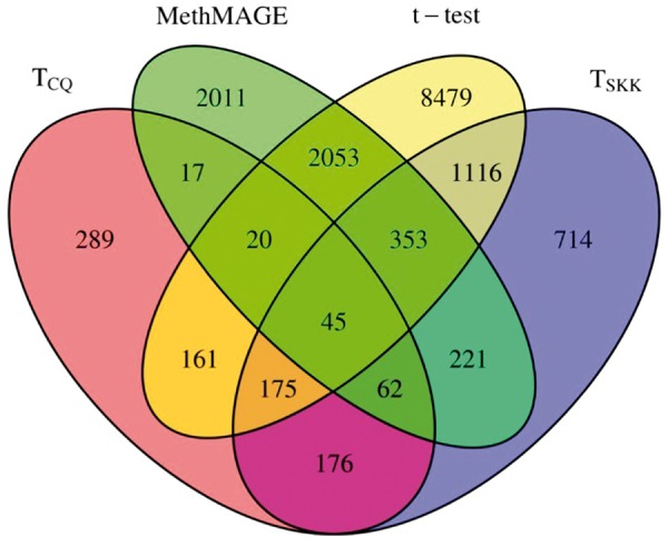
Venn diagram showing the number of regions detected to be differentially methylated by $T_{CQ},\hspace{0.5em}{T}_{SKK},\hspace{0.5em}t$-test and MethMAGE.

Canonical gene pathways constructed using QIAGEN’s Ingenuity Pathway Analysis® (IPA) are presented in Figure 4. Because $t$-test showed extremely high type I error rate, we have performed IPA only for $T_{CQ},\hspace{0.5em}{T}_{SKK}$ and MethMAGE. Using a significance level of $1\%$, we see that $T_{CQ}$ has a higher proportion of pathways detected ($33\%$) to be AML cancer-related when compared with $T_{SKK}$ and MethMAGE ($25\%$). This is consistent with our observations from the simulation study where $T_{CQ}$ has slightly inflated type I error rate but achieves high power, whereas $T_{SKK}$ and MethMAGE were liberal. The high type I error for $T_{SKK}$ and MethMAGE observed in the simulations indicate that most of the pathways detected could potentially be false positives.

Figure 4.

Top-10 canonical pathways produced from the lists of genes that are detected to be significantly differentially methylated in the AML cancer data by the three methods: (A) T_CQ, (B) T_SKK, and (C) MethMAGG.

Results—ovarian data

To analyze the ovarian cancer data, we considered four tests—$T_{SKK},\hspace{0.5em}{T}_{CQ},\hspace{0.5em}{T}_{PA}\hspace{0.5em}\text{and}\hspace{0.5em}t$-test. Owing to large sample size and high number of CG sites in the CpG islands, MethMAGE failed to converge in a considerable amount of time. Hence, we did not consider MethMAGE in our analysis. Figure 5 presents the Venn diagrams for the ovarian recurrence data set where the groups are separated by diagnosis, normalcy and recurrence status, respectively. An interesting feature is the failure of $T_{SKK}$ to detect DMRs when subjects are grouped by recurrence status. In simulation studies based on the ovarian cancer data, $T_{SKK}$ is seen to have inflated type I error rate. We speculate that the failure to identify more than one region as differentially methylated is possibly owing to high bias in the estimation of the correlation matrix.

Figure 5.

Venn diagrams showing the number of regions detected to be differentially methylated by $T_{CQ},\hspace{0.5em}{T}_{PA},\hspace{0.5em}{T}_{SKK}\hspace{0.5em}\text{and}\hspace{0.5em}t$-test method for the ovarian cancer data. The three plots from left to right correspond to data separated based on (A) diagnosis, (B) recurrence and (C) normalcy status.

Biological relevance of DMRs produced when samples are divided by their diagnosis status was explored using the canonical pathways produced by IPA. We used only diagnosis as the group status because it allows us to detect pathways that are different between malignant and benign subjects. As in the AML analysis, as the $t$-test shows extremely high type I error rate and detects almost all the regions as differentially methylated, we have performed IPA only for $T_{CQ},\hspace{0.5em}{T}_{PA}\hspace{0.5em}\text{and}\hspace{0.5em}{T}_{SKK}$. For each of the three methods, the CpG island DMRs were associated with the nearest downstream gene to generate a gene list to be input into IPA. The lists produced by the three methods are presented in Figure 6. The gene list from each method produced a number of overlapping biologically relevant, cancer-related canonical pathways.

Figure 6.

Top-10 canonical pathways produced from the lists of gene lists detected to be significantly differentially methylated in the ovarian cancer data by the three methods: $\left(\text{A}\right)T_{CQ},\hspace{0.5em}\left(\text{B}\right)T_{SKK}$ and $\left(\text{C}\right)T_{PA}$.

All three methods show similar proportion of ovarian-cancer-related pathways detected—$60\%\hspace{0.5em}\text{for}\hspace{0.5em}{T}_{CQ}\hspace{0.5em}\text{and}\hspace{0.5em}50\%\hspace{0.5em}\text{for}\hspace{0.5em}{T}_{SKK}\hspace{0.5em}\text{and}\hspace{0.5em}{T}_{PA}$. However, only genes associated with the DMRs from $T_{CQ}$ resulted in an ovarian-specific pathway (marked by an asterisk) that was significantly enriched. As $T_{CQ}\hspace{0.5em}\text{and}\hspace{0.5em}{T}_{PA}$ were seen to be controlling type I error in simulation studies, it is unlikely that the pathways detected by these methods are false positives.

Conclusions and discussion

In this article, we explored applicability of high-dimensional vector mean testing procedures to detect DMRs using MethylCap-seq data. Using PrEMeR-CG, a probabilistic method for assigning methylation signals to CG sites, we have demonstrated effectiveness of the vector mean tests when compared with the more commonly used $t$-test and MethMAGE. The vector mean tests are developed for a larger family of correlation structures as opposed to MethMAGE. The $t$-test is shown to ignore the correlation structure when averaging or totaling the signal over sites within a region, resulting in extremely inflated type I error rates.

Performance of the mean vector tests is strongly affected by sparsity profiles across samples for the two groups. Hence, we recommend first investigating sparsity of the signals across samples. When the signals observed are sparse, $T_{CQ}$ is seen to be the best test both in terms of controlling type I error and achieving power. $T_{PA}\hspace{0.5em}\text{and}\hspace{0.5em}{T}_{SKK}$ are sensitive to difference between sparsity profiles of the two groups but perform well when the difference is small. Similarity in performance of $T_{PA}$ when the diagonal of covariance matrix is specified to be equal or different is an indication that the site-wise variability of methylation signals is fairly consistent.

For the ovarian cohort simulations where the signals are based on CpG islands, $T_{PA}$ is observed to be conservative, whereas $T_{CQ}$ is seen to have slightly higher type I error rate. This can be attributed to empirical error, as the normal distribution of the test statistic is asymptotic. Although the assumptions made are similar, $T_{SKK}$ fails to control type I error. This might be because of the restriction between sample size and dimension, which is not assumed for $T_{CQ}\hspace{0.5em}\text{and}\hspace{0.5em}{T}_{PA}.\hspace{0.5em}{T}_{CQ}$ attains much higher power than $T_{PA}$ under all models, and because the difference in power between them is much greater than loss in type I error in this trade-off, we conclude that $T_{CQ}$ is the best test for detecting differential methylation in CpG islands.

The above conclusions are drawn based on simulated data sets with samples of 20 and 10 in the two groups. Although these sample sizes are much smaller than the sample sizes for the ovarian data set, they are larger than the AMD data set, and therefore we further evaluate the performance of the tests for simulated data sets with two groups of six and four samples to match the total sample size (10) of the AMD data. However, note that although the AMD data consist of two groups of seven and three samples, we opted for the six and four split in this simulation because $T_{PA}$ requires the minimum of four samples in each group. The results, as presented in Supplementary Tables S7–S10 and Supplementary Figures S10 and S11, show that $T_{CQ}$ continues to outperform the other mean vector tests and MethMAGE. It is noted, though, that the t-test for the simulation based on the AMD data has higher power than $T_{CQ}$ when the empirical type I error is controlled to be at the 5% level under two of the setups. More details are provided in Supplementary Material S4.

In both simulations with 10 DMRs and 10 non-DMRs, the regions were selected from the AMD and the ovarian data according to the following criteria: (1) The number of CG sites in each region should be >50 but <200. This is to have more sites than sample size, but not too large that MethMAGE will not run in a reasonable amount of time. (2) Each region should have at least 40% of its sites with nonzero signal for at least one individual. Because the test statistics remove sites with all zero signals, this is to ensure that a reasonable number of sites remain for the analyses. (3) For the 10 DMRs, we further require that the means are significantly different based on the real data analysis to ensure that the tests will have a good chance of detecting the difference. Nevertheless, we recognize the need to consider other regions in the genome to more comprehensively evaluate the vector mean testing methods. Thus, we carried out an additional simulation study by randomly selecting 200 DMRs and 5000 non-DMRs to further gauge the performances of the methods in a variety, and potentially less ideal, settings of sparsity. However, owing to its computational intensiveness and inferior performance, MethMAGE was not included in this set of simulations. Our findings led to similar conclusions as those based on the more carefully selected regions. That is, $T_{CQ}$ is the method that can best balance type I error and power, and is recommended across all sparsity settings. Details are provided in Supplementary Material S5 and Supplementary Figures S12–S17.

Testing DMR calling methods on actual biological data is hampered by the absence of a definite test data set, in which the true DMRs are known. Nevertheless, it is a promising sign that $T_{CQ}$, when applied to the ovarian data set, identified DMRs with the corresponding genes significantly enriched in an ovarian-specific pathway, while the other methods only identified more generic cancer-related pathways. This indicates that the lower Type I error rate and higher power of $T_{CQ}$ when compared with the other tests on simulated data can indeed identify DMRs that are more likely to be biologically relevant for the system under study.

Software availability

MethylCapSig, the software that implements the five methods studied in this article, is freely available for download at http://www.stat.osu.edu/$\sim$statgen/SOFTWARE/MethylCapSig/ or from CRAN at https://cran.r-project.org/web/packages/MethylCapSig/index.html.

Key Points

• Mean vector tests are better than currently practiced methods at controlling type I error for detecting differentially methylated regions.

• Of all mean vector tests, T_CQ performs the best for methylation signal data and is based on minimal regularity conditions.

• Difference in sparsity profiles should be investigated to validate accuracy of results.

Supplementary Data

Supplementary data are available online at https://academic.oup.com/bib.

Funding

This work was supported in part by grants from the National Science Foundation DMS-1220772 and the National Institute of Health 1R01GM114142-01.

Biographies

Deepak N. Ayyala is postdoctoral researcher, Department of Statistics, The Ohio State University.

David E. Frankhouser is a graduate student.

Javkhlan-Ochir Ganbat is a graduate student.

Guido Marcucci is a Professor, The Ohio State University Wexner Medical Center.

Ralf Bundschuh is a Professor, The Ohio State University Wexner Medical Center.

Pearlly Yan is a Professor, The Ohio State University Wexner Medical Center.

Shili Lin is a Professor, Department of Statistics, The Ohio State University.

References

- 1.Frommer M, McDonald LE, Millar DS, et al. A genomic sequencing protocol that yields a positive display of 5-methylcytosine residues in individual DNA strands. Proc Natl Acad Sci USA 1992;89:1827–31. [DOI] [PMC free article] [PubMed] [Google Scholar]
- 2.Lister R, Pelizolla M, Dowen RH, et al. Human DNA methylomes at base resolution show widespread epigenomic differences. Nature 2009;462:315–22. [DOI] [PMC free article] [PubMed] [Google Scholar]
- 3.Meissner A, Gnirke A, Bell GW, et al. Reduced representation bisulfite sequencing for comparative high-resolution DNA methylation analysis. Nucleic Acids Res 2005;33(18):5868–77. [DOI] [PMC free article] [PubMed] [Google Scholar]
- 4.Weber M, Davies JJ, Wittig D, et al. Chromosome-wide and promoter-specific analyses identify sites of differential DNA methylation in normal and transformed human cells. Nat Genet 2005;37(8):853–62. [DOI] [PubMed] [Google Scholar]
- 5.Frankhouser DE, Murphy M, Blachly JS, et al. PrEMeR-CG: inferring nucleotide level DNA methylation values from MethylCap-seq data. Bioinformatics 2014;30(24):3567–74. [DOI] [PMC free article] [PubMed] [Google Scholar]
- 6.Taiwo O, Wilson GA, Morris T, et al. Methylome analysis using MeDIP-seq with low DNA concentrations. Nat Protoc 2012;7:617–36. [DOI] [PubMed] [Google Scholar]
- 7.Eckhardt F, Lewin J, Cortese R, et al. DNA methylation profiling of human chromosomes 6, 20 and 22. Nat Genet 2006;38:1378–85. [DOI] [PMC free article] [PubMed] [Google Scholar]
- 8.Kuan PF, Chiang DY. Integrating prior knowledge in multiple testing under dependence with applications to detecting differential DNA methylation. Biometrics 2012;68:774–83. [DOI] [PMC free article] [PubMed] [Google Scholar]
- 9.Chavez L, Lienhard M, Dietrich J. MEDIPS: (MeD)IP-seq data analysis. R package version 1.16.0. 2013. www.biocondutor.org/packages/release/bioc/html/MEDIPS.html. [Google Scholar]
- 10.Bock C, Tomazou EM, Brinkman AB, et al. Genome-wide mapping of DNA methylation: a quantitative technology comparison. Nat Biotechnol 2010;28:1106–14. [DOI] [PMC free article] [PubMed] [Google Scholar]
- 11.Carvalho RH, Haberle V, Hou J, et al. Genome-wide DNA methylation profiling of non-small cell lung carcinomas. Epigenet Chromatin 2012;5(1):9. [DOI] [PMC free article] [PubMed] [Google Scholar]
- 12.Carvalho RH, Hou J, Haberle V, et al. Genomewide DNA methylation analysis identifies novel methylated genes in non-small-cell lung carcinomas. J Thorac Oncol 2013;8(5):562–73. [DOI] [PubMed] [Google Scholar]
- 13.Zhao Y, Guo S, Sun J, et al. Methylcap-Seq reveals novel DNA methylation markers for the diagnosis and recurrence prediction of bladder cancer in a Chinese population. PLoS One 2012;7(4):e35175. [DOI] [PMC free article] [PubMed] [Google Scholar]
- 14.Lendvai A, Johannes F, Grimm C, et al. Genome-wide methylation profiling identifies hypermethylated biomarkers in high-grade cervical intraepithelial neoplasia. Epigenetics 2012;7(11):1268–78. [DOI] [PMC free article] [PubMed] [Google Scholar]
- 15.Feng H, Conneely KN, Wu H. A Bayesian hierarchical model to detect differentially methylated loci from single nucleotide resolution sequencing data. Nucleic Acids Res 2014;42:e69. [DOI] [PMC free article] [PubMed] [Google Scholar]
- 16.Hansen KD, Langmead B, Irizarry RA. BSmooth: from whole genome bisulfite sequencing reads to differentially methylated regions. Genome Biol 2012;13:R83. [DOI] [PMC free article] [PubMed] [Google Scholar]
- 17.Park Y, Figueroa ME, Rozek LS, et al. methylSig: a whole genome DNA methylation analysis pipeline. Bioinformatics 2014;30:2414–22. [DOI] [PMC free article] [PubMed] [Google Scholar]
- 18.Yan P, Frankhouser D, Murphy M, et al. Genome-wide methylation profiling in decibatine-treated patients with acute myeloid leukemia. Blood 2012;120(12):2466–74. [DOI] [PMC free article] [PubMed] [Google Scholar]
- 19.Chen SX, Qin Y. A two-sample test for high-dimensional data with applications to gene-set testing. Ann Stat 2010;38:808–35. [Google Scholar]
- 20.Park J, Ayyala DN. A test for the mean vector in large dimension and small samples. J Stati Plan Inference 2013;143:929–43. [Google Scholar]
- 21.Srivastava MS, Katayama S, Kano Y. A two sample test in high dimensional data. J Multivar Anal 2013;114:349–58. [Google Scholar]
- 22.Bai Z, Saranadasa H. Effect of high dimension: by an example of a two sample problem. Stat Sinica 1996;6:311–29. [Google Scholar]
- 23.Dempster AP. A high dimensional two sample significance test. Ann Math Stat 1958;29(4):995–1010. [Google Scholar]
- 24.Jaffe AE, Feinberg AP, Irizarry RA, et al. Significance analysis and statistical dissection of variably methylated regions. Biostatistics 2012;13(1):166–78. [DOI] [PMC free article] [PubMed] [Google Scholar]
- 25.Huang R, Gu F, Kirma NB, et al. Comprehensive methylome analysis of ovarian tumors reveals hedgehog signaling pathway regulators as prognostic DNA methylation biomarkers. Epigenetics 2013;8(6):624–34. [DOI] [PMC free article] [PubMed] [Google Scholar]
Associated Data
This section collects any data citations, data availability statements, or supplementary materials included in this article.