Postgenomics: Proteomics and Bioinformatics in Cancer Research

Abstract

Now that the human genome is completed, the characterization of the proteins encoded by the sequence remains a challenging task. The study of the complete protein complement of the genome, the “proteome,” referred to as proteomics, will be essential if new therapeutic drugs and new disease biomarkers for early diagnosis are to be developed. Research efforts are already underway to develop the technology necessary to compare the specific protein profiles of diseased versus nondiseased states. These technologies provide a wealth of information and rapidly generate large quantities of data. Processing the large amounts of data will lead to useful predictive mathematical descriptions of biological systems which will permit rapid identification of novel therapeutic targets and identification of metabolic disorders. Here, we present an overview of the current status and future research approaches in defining the cancer cell's proteome in combination with different bioinformatics and computational biology tools toward a better understanding of health and disease.

TECHNOLOGIES FOR PROTEOMICS

2D gel electrophoresis

Two-dimensional gel electrophoresis (2DE) is by far the most widely used tool in proteomics approaches for more than 25 years [1]. This technique involves the separation of complex mixtures of proteins first on the basis of isoelectric point (pI) using isoelectric focusing (IEF) and then in a second dimension based on molecular mass. The proteins are separated by migration in a polyacrylamide gel. By use of different gel staining techniques such as silver staining [2], Coomassie blue stain, fluorescent dyes [3], or radiolabels, few thousands proteins can be visualized on a single gel. Fluorescent dyes are being developed to overcome some of the drawbacks of silver staining in making the protein samples more amenable to mass spectrometry [4, 5]. Stained gels can then be scanned at different resolutions with laser densitometers, fluorescent imager, or other device. The data can be analyzed with software such as PDQuest by Bio-Rad Laboratories (Hercules, Calif, USA) [6], Melanie 3 by GeneBio (Geneva, Switzerland), Imagemaster 2D Elite by Amersham Biosciences, and DeCyder 2D Analysis by Amersham Biosciences (Buckinghamshire, UK) [7]. Ratio analysis is used to detect quantitative changes in proteins between two samples. 2DE is currently being adapted to high-throughput platforms [8]. For setting up a high-throughput environment for proteome analysis, it is essential that the 2D gel image analysis software supports robust database tools for sorting images, as well as data from spot analysis, quantification, and identification.

ProteinChips

While proteomics has become almost synonymous with 2D gel electrophoresis, there is a variety of new methods for proteome analysis. Unique ionization techniques, such as electrospray ionization and matrix-assisted laser desorption-ionization (MALDI), have facilitated the characterization of proteins by mass spectrometry (MS) [9, 10]. These techniques have enabled the transfer of the proteins into the gas phase, making it conducive for their analysis in the mass spectrometer. Typically, sequence-specific proteases are used to break up the proteins into peptides that are coprecipitated with a light-absorbing matrix such as dihydroxy benzoic acid. The peptides are then subjected to short pulses of ultraviolet radiation under reduced pressure. Some of the peptides are ionized and accelerated in an electric field and subsequently turned back through an energy correction device [11]. Peptide mass is derived through a time-of-flight (TOF) measurement of the elapsed time from acceleration-to-field free drift or through a quadrupole detector. A peptide mass map is generated with the sensitivity to detect molecules at a few parts per million. Hence a spectrum is generated with the molecular mass of individual peptides, which are used to search databases to find matching proteins. A minimum of three peptide molecular weights is necessary to minimize false-positive matches. The principle behind peptide mass mapping is the matching of experimentally generated peptides with those determined for each entry in a sequence. The alternative process of ionization, through the electrospray ionization, involves dispersion of the sample through a capillary device at high voltage [11]. The charged peptides pass through a mass spectrometer under reduced pressure and are separated according to their mass-to-charge ratios through electric fields. After separation through 2DE, digested peptide samples can be delivered to the mass spectrometer through a “nanoelectrospray” or directly from a liquid chromatography column (liquid chromatography-MS), allowing for real-time sequencing and identification of proteins. Recent developments have led to the MALDI quadrupole TOF instrument, which combines peptide mapping with peptide sequencing approach [12, 13, 14]. An important feature of tandem MS (MS-MS) analysis is the ability to accurately identify posttranslational modifications, such as phosphorylation and glycosylation, through the measurement of mass shifts.

Another MS-based proteinChip technology, surface-enhanced laser desorption-ionization time of flight mass spectrometry (SELDI-TOF-MS), has been successfully used to detect several disease-associated proteins in complex biological specimens, such as cell lysates, seminal plasma, and serum [15, 16, 17]. Surface-enhanced laser desorption-ionization (SELDI) is an affinity-based MS method in which proteins are selectively adsorbed to a chemically modified surface, and impurities are removed by washing with buffer. The use of several different chromatographic arrays and wash conditions enables high-speed, high-resolution chromatographic separations [14].

Other technologies

Arrays of peptides and proteins provide another bio-chip strategy for parallel protein analysis. Protein assays using ordered arrays have been explored through the development of multipin synthesis [18]. Arrays of clones from phage-display libraries can be probed with antigen-coated filters for high-throughput antibody screening [19]. Proteins covalently attached to glass slides through aldehyde-containing silane reagents have been used to detect protein-protein interactions, enzymatic targets, and protein small molecule interactions [20]. Other methods of generating protein microarrays are by printing the proteins (ie, purified proteins, recombinant proteins, and crude mixtures) or antibodies using a robotic arrayer and a coated microscope slide in an ordered array. Protein solutions to be measured are labeled by covalent linkage of a fluorescent dye to the amino groups on the proteins [21]. Protein arrays consisting of immobilized proteins from pure populations of microdissected cells have been used to identify and track cancer progression. Although protein arrays hold considerable promise for functional proteomics and expression profiling for monitoring a disease state, certain limitations need to be overcome. These include the development of high-throughput technologies to express and purify proteins and the generation of large sets of well-characterized antibodies. Generating protein and antibody arrays is more costly and labor-intensive relative to DNA arrays. Nevertheless, the availability of large antibody arrays would enhance the discovery of differential biomarkers in nondiseased and cancer tissue [22].

Tissue arrays have been developed for high-throughput molecular profiling of tumor specimens [23]. Arrays are generated by robotic punching out of small cylinders (0.6 mm × 3—4 mm high) of tissue from thousands of individual tumor specimens embedded in paraffin to array them in a paraffin block. Tissue from as many as 600 specimens can be represented in a single “master” paraffin block. By use of serial sections of the tissue array, tumors can be analyzed in parallel by immunohistochemistry, fluorescence in situ hybridization, and RNA-RNA in situ hybridization. Tissue arrays have applications in the simultaneous analysis of tumors from many different patients at different stages of disease. Disadvantages of this technique are that a single core is not representative because of tumor heterogeneity and uncertainty of antigen stability on long-term storage of the array. Hoos et al [24] demonstrated that using triplicate cores per tumor led to lower numbers of lost cases and lower nonconcordance with typical full sections relative to one or two cores per tumor. Camp et al [25] found no antigenic loss after storage of an array for 3 months. Validation of tissue microarrays is currently ongoing in breast and prostate cancers and will undoubtedly help in protein expression profiling [23, 25, 26]. A major advantage of this technology is that expression profiles can be correlated with outcomes from large cohorts in a matter of few days.

PROTEOMICS IN CANCER RESEARCH

Cancer proteomics encompasses the identification and quantitative analysis of differentially expressed proteins relative to healthy tissue counterparts at different stages of disease, from preneoplasia to neoplasia. Proteomic technologies can also be used to identify markers for cancer diagnosis, to monitor disease progression, and to identify therapeutic targets. Proteomics is valuable in the discovery of biomarkers because the proteome reflects both the intrinsic genetic program of the cell and the impact of its immediate environment. Protein expression and function are subject to modulation through transcription as well as through posttranscriptional and posttranslational events. More than one RNA can result from one gene through a process of differential splicing. Additionally, there are more than 200 posttranslation modifications that proteins could undergo, that affect function, protein-protein and nuclide-protein interaction, stability, targeting, half-life, and so on [27], all contributing to a potentially large number of protein products from one gene. At the protein level, distinct changes occur during the transformation of a healthy cell into a neoplastic cell, ranging from altered expression, differential protein modification, and changes in specific activity, to aberrant localization, all of which may affect cellular function. Identifying and understanding these changes are the underlying themes in cancer proteomics. The deliverables include identification of biomarkers that have utility both for early detection and for determining of therapy.

Although proteomics traditionally dealt with quantitative analysis of protein expression, more recently, proteomics has been viewed to encompass the structural analysis of proteins [28]. Quantitative proteomics strives to investigate the changes in protein expression in different states, such as in healthy and diseased tissue or at different stages of the disease. This enables the identification of state- and stage-specific proteins. Structural proteomics attempts to uncover the structure of proteins and to unravel and map protein-protein interactions.

MS has been helpful in the analysis of proteins from cancer tissues. Screening for the multiple forms of the molecular chaperone 14-3-3 protein in healthy breast epithelial cells and breast carcinomas yielded a potential marker for the noncancerous cells [29]. The 14-3-3 form was observed to be strongly down regulated in primary breast carcinomas and breast cancer cell lines relative to healthy breast epithelial cells. This finding, in the light of the evidence that the gene for 14-3-3 was found silenced in breast cancer cells [30], implicates this protein as a tumor suppressor. Using a MALDI-MS system, Bergman et al [6] detected increases in the expressions of nuclear matrix, redox, and cytoskeletal proteins in breast carcinoma relative to benign tumors. Fibroadenoma exhibited an increase in the oncogene product DJ-1. Retinoic acid-binding protein, carbohydrate-binding protein, and certain lipoproteins were increased in ovarian carcinoma, whereas cathepsin D was increased in lung adenocarcinoma.

Imaging MS is a new technology for direct mapping and imaging of biomolecules present in tissue sections. For this system, frozen tissue sections or individual cells are mounted on a metal plate, coated with ultraviolet-absorbing matrix, and placed in the MS. With the use of an optical scanning raster over the tissue specimen and measurement of the peak intensities over thousands of spots, MS images are generated at specific mass values [31]. Stoeckli et al [32] used imaging MS to examine protein expression in sections of human glioblastoma and found increased expression of several proteins in the proliferating area compared with healthy tissue. Liquid chromatography—MS and tandem MS (MS-MS) were used to identify thymosin ß.4, a 4964-d protein found only in the outer proliferating zone of the tumor [32]. Imaging MS shows potential for several applications, including biomarker discovery, biomarker tissue localization, understanding of the molecular complexities of tumor cells, and intraoperative assessment of surgical margins of tumors.

SELDI, originally described by Hutchens and Yip [33], overcomes many of the problems associated with sample preparations inherent with MALDI-MS. The underlying principle in SELDI is surface-enhanced affinity capture through the use of specific probe surfaces or chips. This protein biochip is the counterpart of the array technology in the genomic field and also forms the platform for Ciphergen's ProteinChip array SELDI MS system [14]. A 2DE analysis separation is not necessary for SELDI analysis because it can bind protein molecules on the basis of its defined chip surfaces. Chips with broad binding properties, including immobilized metal affinity capture, and with biochemically characterized surfaces, such as antibodies and receptors, form the core of SELDI. This MS technology enables both biomarker discovery and protein profiling directly from the sample source without preprocessing. Sample volumes can be scaled down to as low as 0.5 μL, an advantage in cases in which sample volume is limiting. Once captured on the SELDI protein biochip array, proteins are detected through the ionization-desorption TOF-MS process. A retentate (proteins retained on the chip) map is generated in which the individual proteins are displayed as separate peaks on the basis of their mass and charge (m/z). Wright et al [15] demonstrated the utility of the ProteinChip SELDI-MS in identifying known markers of prostate cancer and in discovering potential markers either over- or underexpressed in prostate cancer cells and body fluids. SELDI analyses of cell lysates prepared from pure populations from microdissected surgical tissue specimens revealed differentially expressed proteins in the cancer cell lysate when compared with healthy cell lysates and with benign prostatic hyperplasia (BPH) and prostate intraepithelial neoplasia cell lysates [15]. SELDI is a method that provides protein profiles or patterns in a short period of time from a small starting sample, suggesting that molecular fingerprints may provide insights into changing protein expression from healthy to benign to premalignant to malignant lesions. This appears to be the case because distinct SELDI protein profiles for each cell and cancer type evaluated, including prostate, lung, ovarian, and breast cancer, have been described recently [34, 35]. After prefractionation, a SELDI profile of 30 dysregulated proteins was observed in seminal plasma from prostate cancer patients. One of the seminal plasma proteins detected by comparing the prostate cancer profiles with a BPH profile was identified as seminal basic protein, a proteolytic product of semenogelin I [14].

BIOINFORMATICS TOOLS

Bioinformatics tools are needed at all levels of proteomic analysis. The main databases serving as the targets for MS data searches are the expressed sequence tag and the protein sequence databases, which contain protein sequence information translated from DNA sequence data [11]. It is thought that virtually any protein that can be detected on a 2D gel can be identified through the expressed sequence tag database, which contains over 2 million cDNA sequences [36]. A modification of sequence-tag algorithms has been shown to locate peptides given the fact that the expressed sequence tags cover only a partial sequence of the protein [37].

Data mining for proteomics

A number of algorithms have been proposed for genomes-scale analysis of patterns of gene expression, including expressed sequence tags (ESTs) (simple expedient of counting), UniGene for gene indexes [38]. Going beyond expression data, efforts in proteomics can be expressed to fill in a more complete picture of posttranscriptional events and the overall protein content of cells. To address the large-in-scale data, this review addresses primarily those advances in recent years.

Concurrent to the development of the genome sequences for many organisms, MS has become a valuable technique for the rapid identification of proteins and is now a standard more sensitive and much faster alternative to the more traditional approaches to sequencing such as Edman degradation.

Due to the large array of data that is generated from a single analysis, it is essential to implement the use of algorithms that can detect expression patterns from such large volumes of data correlating to a given biological/pathological phenotype from multiple samples. It enables the identification of validated biomarkers correlating strongly to disease progression. This would not only classify the cancerous and noncancerous tissues according to their molecular profile but could also focus attention upon a relatively small number of molecules that might warrant further biochemical/molecular characterization to assess their suitability as potential therapeutic targets. Data screened is usually of large size and has about 100 000–120 000 variables.

Biologists are not prepared to handle the huge data produced by the proteins or DNA microarray projects or to use the “eye” to visualize and interpret the output, therefore to detect pattern, visualize, classify, and store the data, more sophisticated tools are needed. Bioinformatics has proved to be a powerful tool in the effective generation of primarily predictive proteomic data from analysis of DNA sequences. Proteomics studies applications and techniques, includes profiling expression patterns in response to various variables and conditions and time correlation analysis of protein expression.

Intelligent data mining facilities are essential if we are to prevent important results from being lost in the mass of information. The analysis of data can proceed with different levels. One level of differential analysis where genes are analyzed one by one independently of each other to detect changes in expression across different conditions. This is challenging due to the amount of noise involved and low repetition characteristic of microarray experiments. The next level of analysis involves visualizing and feature discovery. Basic statistical tools and statistical inferences include cluster analysis, Bayesian modeling, classification, and discrimination, neural networks, and graphical models. The basic idea behind those approaches is to visualize the correlations in the data to allow the data to be examined for similarity and detection of important expression patterns (principal component analysis) to learn (classification, neural networks, support vector machine), to predict (prediction, regression, regression tree), to detect feature discovery, and to test hypotheses regarding the number of distinct clusters contained within the data (hierarchical clustering, Bayesian clustering, k-means, mixture model with Gibbs sampler or EM algorithm).

These algorithms can quickly analyze gels to identify how a series of gels are related, for example, confirming separation of clusters into healthy (control), diseased, and treatments clusters, or perhaps pointing to the existence of a cluster which has not previously been considered, which is a population of cells exhibiting drug resistance [39, 40].

Principal component analysis

Principal component analysis (PCA) can be an effective method of identifying the most discriminating features in a data set. This technique usually involves finding two or three linear combinations of the original features that best summarize the types of variation in the data. If much of the variation is captured by these two or three most significant principal components, class membership of many data points can be observed. One may use the principal-component solution to the factor model for extracting factors (components). This is accomplished by the use of the principal-axis theorem, which says that for a gene-by-gene (n × n) correlation matrix R, there exists a rotation matrix D and diagonal matrix Λ such that DRD ^t = Λ. The principal form of R is given as

(1)

where columns of D and D ^t are the eigenvectors and diagonal entries of Λ are the eigenvalues. Components whose eigenvalues exceed unity, λ _j > 1, are extracted from Λ and sorted such that λ₁ ≥ λ₂ ≥ ⋯ ≥ λ _m ≥ 1. The “loading” or correlation between genes and extracted components is represented by a matrix in the form

(2)

where rows represent genes and columns represent components, and, for example, √λ₁d₁₁ is the loading (correlation) between gene 1 and component 1. CLUSFAVOR algorithm proposed by Leif [41] performs PCA along with hierarchical clustering (see “Hierarchical clustering and decision tree” section) with DNA microarray expression data. CLUSFAVOR standardizes expression data and sorts and performs hierarchical and PCA of arrays and genes. Applying CLUSFAVOR, principal component method is used and component extraction and loading calculations are completed, a varimax orthogonal rotation of components is completed so that each gene mostly loads on a single component [42]. The result reported in [41] mixing hierarchical clustering and PCS was summarized through a colored tree, where genes that load strongly negative (less than −0.45) or strongly positive (greater than 0.45) on a single component are indicated by the use of two arbitrary colors in the column for each component whereas genes with identical color patterns in one or more columns were considered as having similar expression profiles within the selected group of genes.

Unsupervised learning based on normal mixture models

Unsupervised clustering is used to detect pattern, feature discovery, and also to match the protein sequence to the database sequences. Unsupervised learning enables pattern discovery by organizing data into clusters, using recursive partitioning methods. In the last 25 years it has been found that basing cluster analysis on a probability model can be useful both for understanding when existing methods are likely to be successful and for suggesting new methods [43, 44, 45, 46, 47, 48, 49]. One such probability model is that the population of interest consists of K different subpopulations G₁,⋯,G_K and that the density of a p-dimensional observation x from the kth subpopulation is f_k (x,θ_k ) for some unknown vector of parameters θ_k (k = 1, ⋯, K). Given observations x = (x ₁, ⋯, x _n ), we let ν = (ν₁, ⋯, ν _n ) ^t denote the unknown identifying labels, where ν _i = k if x _i comes from the kth subpopulation. In the so-called classification maximum likelihood procedure, θ = (θ ₁, ⋯, θ _K ) and ν = (ν₁, ⋯, ν _n ) ^t are chosen to maximize the classification likelihood:

(3)

Normal mixture is a traditional statistical tool which has successfully been applied in gene expression [50]. For multivariate data of a continuous nature, attention has focused on the use of multivariate normal components because of their computational convenience. In this case, the data x = (x ₁, ⋯, x _n ) to be classified are viewed as coming from a mixture of probability distributions, each representing a different cluster, so the likelihood is expressed as

(4)

where π_k is the probability that an observation belongs to the kth components (π _k ≥ 0;  ∑ _{k = 1} ^k π _k = 1).

In the theory of finite mixture, recently, methods based on this theory performed well in many cases and applications including character recognition [51], tissue segmentation [52], application to astronomical data [53, 54, 55] and enzymatic activity in the blood [56].

Once the mixture is fitted, a probabilistic clustering of the data into a certain number of clusters can be obtained in terms of the fitted posterior probabilities of component membership for the data. The likelihood ratio statistic, Bayesian information criteria (BIC), Akaike information criteria (AIC), information complexity criteria (ICOMP), and others are used to choose the number of clusters if there is any. A mixture of t-distribution may also be used instead of mixture of normals in order to provide some protection against atypical observations, which are prevalent in microarray data.

McLachlan et al [50] proposed a model-based approach to the clustering of tissue samples on a very large number of genes. They first select a subset of genes relevant for the clustering of the tissue samples by fitting mixtures of t distributions to rank the genes in order of increasing size of the likelihood ratio statistic for the test of one versus two components in the mixture model. The use of t component distributions was employed in the gene selection in order to provide some protection against atypical observations, which exit in genomics and proteomics data. In this case, the data x to be classified is viewed as coming from a mixture of probability distributions (4), where f_k (x |θ _k = (μ_k ,Σ _k , γ _k )) is a t density with location μ _k , positive definite inner product matrix Σ _k , and γ _k degrees of freedom is given by

(5)

where δ(x, μ _k ; Σ _k ) = (x − μ _k ) ^t Σ _k (x − μ _k ) denotes the Mahalanobis squared distance between x and μ _k . If γ _k > 1, μ _k is the mean of x and γ _k > 2, γ _k (γ _k − 2)^{− 1} Σ _k is its covariance matrix.

McLachlan approach was demonstrated on two well-known data sets on colon and leukemia tissues. The algorithm proposed is used to select relevant genes for clustering the tissue samples into two clusters corresponding to healthy and unhealthy tissues.

Weighted voting (WV)

The weighted voting (WV) algorithm directly applies the signal-to-noise ratio to perform binary classification. For a chosen feature x of a test sample, it measures its distance with respect to decision boundary b = (1/2) (μ ₁ + μ ₂), which is located halfway between the average expression levels of two classes, where μ ₁ and μ ₂ are the centers of the two clusters. If the value of this feature falls on one side of the boundary, a vote is added to the corresponding class. The vote V(x) = P(g, c) (x − b) is weighted by the distance between the feature value and the decision boundary and the signal-to-noise ratio of this feature determined by the training set. The vote for each class is computed by summing up the weighted votes, V(x), made by selected features for this class. In this contest, Yeang et al [58] performed multiclass classification by combining the outputs of binary classifiers. Three classifiers including weighted voting were applied over 190 samples from 14 tumor classes where a combined expression dataset was generated. Weighted Voting is a classification tool which, based on the already known clusters, proposes a rule of classification of the data set and then predicts the allocation of new samples to one of the established clusters.

k-nearest neighbors (kNN)

The kNN algorithm is a popular instance-based method of cluster analysis. The algorithm partitions data into a predetermined number of categories as instances are examined, according to a distance measure (eg, Euclidean). Category centroids are fixed at random positions when the model is initialized, which can affect the clustering outcome.

kNN is popular because of its simplicity. It is widely used in machine learning and has numerous variations [57]. Given a test sample of unknown label, it finds the k nearest neighbors in the training set and assigns the label of the test sample according to the labels of those neighbors. The vote from each neighbor is weighted by its rank in terms of the distance to the test sample.

Let G _m = (g _1m , g _2m , ⋯, g _qm ), where g _im is the log expression ratio of the ith gene in the mth specimen; m = 1, ⋯, M (M = number of samples in the training set). In the kNN method, one computes the Euclidean distance between each specimen, represented by its vector G _m , and each of the other specimens. Each specimen is classified according to the class membership of its k-nearest neighbors. In a study undertaken by Hamadeh et al [59], the training set comprised of RNA samples derived from livers of Sprague-Dawley rats exposed to one of 3 peroxisome proliferations. In this study, M = 27, q = 30, and k = 3. A set of q (q = 30) genes was considered discriminative when at least 25 out of 27 specimens were correctly classified. A total of 10,000 such subsets of genes were obtained. Genes were then rank-ordered according to how many times they were selected into these subsets. The top 100 genes were subsequently used for prediction purposes.

kNN can also be used for recovering missing values in DNA microarray. In fact, hundreds of genes can be observed in one particular experiment. Arrays are printed with approximately 1 kilobase of DNA, corresponding to the coding region of a particular gene, per spot. Labelling of cDNA is done to determine where hybridization occurs. Hybridization is viewed either by fluorescence or radioactive intensity. One drawback of these techniques is the scanning of hybridization intensities. A certain threshold value must be met in order for a value to be returned as a valid measurement. If a value is below this threshold, it is returned as missing data. This missing data disrupts the analysis of the experiment. For instance, if a gene is printed in a duplicate, over a series of arrays, and one spot on one array is below the threshold, the gene is disregarded across all arrays. The loss of this gene expression data is costly because no experimental conclusions can be made from the loss of expression of this gene over all arrays [60].

Artificial neural network (ANN)

Unsupervised neural networks provide a more robust and accurate approach to the clustering of large amounts of noisy data. Neural networks have a series of properties that make them suitable for the analysis of gene expression and proteins patterns. They can deal with real-world data sets containing noisy, ill-defined items with irrelevant variables and outliers, and whose statistical distribution does not need to be parametric. Multilayer perceptrons [61] provide a nonlinear mapping where the real-valued input x is transformed and mapped to get a real-valued output y:

(6)

where W is the weight matrix, called first layer, h is a nonlinear transformation, y is a finished node. The following is an example of a two-layer neural network:

(7)

if 0 < y < 1, then we have a classification case with two groups. Technically, classification, for example, is achieved by comparing y = h(x) with a threshold, we suppose here 0 for simplicity, if h(x) > 0, observation x belongs to the cluster 1, if h(x) < 0, then x belongs to cluster 2. The weights W are estimated by examining the training points sequentially.

ANN has been applied to a number of diverse areas for the identification of “biologically relevant” molecules, including pyrolysis mass spectrometry [62] and genomics microarraying of tumor tissue [63]. Ball et al [64] utilized a multilayer perceptron with a back propagation algorithm for the analysis of SELDI mass spectrometry data. This type of ANN is a powerful tool for the analysis of complex data [65]. Wei et al [66] used the same algorithm for data containing a high background noise. ANN can be used to identify the influence of many interacting factors [67] that makes it highly suitable for the study of first-generation SELDI-derived data. It can be used for the classification of human tumors and rapid identification of potential biomarkers [64]. ANN can produce generalized models with a greater accuracy than conventional statistical techniques in medical diagnostics [68, 69] without relying on predetermined relationships as in other modeling techniques. Usually, the data needs to be trained when using ANN to predict tumor grade; also the choice of the number of layers has to be proposed. Currently, ANN does not propose criteria for choosing the number of layers which should be investigator-proposed. A criteria has to be developed for the ANN to choose the adequate number of layers.

For the probabilistic modeling, usually the normality is assumed, whereas in the ANN the data is distribution-free, which makes the ANN a powerful tool for data analysis [70].

Hierarchical clustering and decision tree

The basic idea of the tree is to partition the input space recursively into two halves and approximate the function in each half by the average output value of the samples it contains [71]. Each bifurcation is parallel to one of the axes and can be expressed as an inequality involving the input components (eg, x _k > a). The input space is divided into hypertangles organized into a binary tree where each branch is determined by the dimension (k) and boundary (a) which together minimize the residual error between model and data.

Example

In a study undertaken by Robert Dillman at the University of California, San Diego Cancer Center [72], 21 continuous laboratory variables related to immunocompetence, age, sex, and smoking habits in an attempt to distinguish patient with cancer. Prior probabilities are chosen to be equal: π (1) = π (2) = 0.5, and C(1|2), the cost of misclassification, was calculated. The tree in Figure 1 summarizes the classification of 128 observations into two classes: supposedly healthy and unhealthy.

Figure 1.

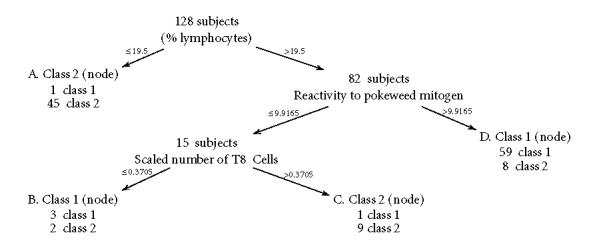
An example of neural network black box: a four-dimensional data input x is first transformed by W, then by h in order to give a grouping variable y as an output.

Currently, hierarchical clustering is the most popular technique employed for microarray data analysis and gene expression [73]. Hierarchical methods are based on building a distance matrix summarizing all the pairwise similarities between expression profiles, and then generating cluster trees (also called dendrograms) from this matrix. Genes which appear to be coexpressed at various time points are positioned close to one another in the tree whose branches lengths represent the degree of similarity between expression profiles.

Decision trees [74] were used to classify proteins as either soluble or insoluble, based on features of their amino acid sequences. Useful rules relating these features with protein solubility were then determined by tracing the paths through the decision trees. Protein solubility strongly influences whether a given protein is a feasible target for structure determination, so the ability to predict this property can be a valuable asset in the optimization of high-throughput projects. These techniques have already been applied to the study of gene expression patterns [73]. Neverthless, classical hierarchical clustering presents drawbacks when dealing with data containing a nonnegligible amount of noise. Hierarchical clustering suffers from a lack of robustness and solutions may not be unique and dependent on the data order. Also, the deterministic nature of hierarchical clustering and the impossibility of re-evaluating the results in the light of the complete data can cause some clusters of patterns to be based on local decisions rather than on the global picture.

Self-organizing mapping (SOM)

The self-organizing feature map (SOM) [75] consists of a neural network whose nodes move in relation to category membership. As with k-means, a distance measure is computed to determine the closest category centroid. Unlike k-means, this category is represented by a node with an associated weight vector. The weight vector of the matching node, along with those of neighboring nodes, is updated to more closely match the input vector. As data points are clustered and category centroids are updated, the positions of neighboring nodes move in relation to them. The number of network nodes which constitute this neighborhood typically decreases over time. The input space is defined by the experimental input data, whereas the output space consists of a set of nodes arranged according to certain topologies, usually two-dimensional grids. The application of the algorithm maps the input space onto the smaller output space, producing a reduction in the complexity of the analyzed data set [76, 77]. Like PCA, the SOM is capable of reducing high-dimensional data into a 1- or 2-dimensional representation. The algorithm produces a topology-preserving map, conserving the relationships among data points. Thus, although either method may be used to effectively partition the input space into clusters of similar data points, the SOM can also indicate relationships between clusters.

SOM is reasonably fast and can be easily scaled to large data sets. They can also provide a partial structure of clusters that facilitate the interpretation of the results. SOM structure, unlike the case of hierarchical cluster, is a two-dimensional grid usually of hexagonal or rectangular geometry, having a number of nodes fixed from the beginning. The nodes of the network are initially random patterns. During the training process, that implies slight changes in the nodes after repeated comparison with the data set, the node changes in a way that captures the distribution of variability of the data set. In this way, similar gene, peak, protein profile patterns map close together in the network and, as far as possible from the different patterns.

A combination of SOM and decision tree was proposed by Herrero et al [78]. The description of the algorithm is given as follows: given the patterns of expression that has to be classified, if two genes are described by their expression patterns as g ₁(e ₁₁, e ₁₂, ⋯, e _1n ) and g ₂(e ₂₁, e ₂₂, ⋯, e _2n ) and their distance d _1,2 = √∑ (e _1i − e _2i )², the initial system of the SOM is composed of two external elements, connected by an internal element. Each cell is a vector with the same size as the gene profiles. The entries of the two cells and the node are initialized. The network is trained only through their terminal neurons or cells. The algorithm proceeds by expanding the output topology starting from the cell having the most heterogeneous population of associated input gene profiles. Two new descendents are generated from this heterogeneous cell that changes its state from cell to node. The series of operations performed until a cell generates two descendents is called a cycle. During a cycle, cells and nodes are repeatedly adapted by the input gene profiles. This process of successive cycles of generation of descendant cells can last until each cell has one single input gene profile assigned (or several, identical profiles), producing a complete classification of all the gene profiles. Alternatively, the expansion can be stopped at the desired level of heterogeneity in the cells, producing in this way a classification of profiles at a higher hierarchical level.

Kanaya et al [79] use SOM to efficiently and comprehensively analyze codon usage in approximately 60,000 genes from 29 bacterial species simultaneously. They showed that SOM is an efficient tool for characterizing horizontally transferred genes and predicting the donor/acceptor relationship with respect to the transferred genes. They examined codon usage heterogeneity in the E coli O 157 genome, which contains the unique segments including O-islands [81] that are absent in E coli K 12.

Support vector machine (SVM)

SVM originally introduced by Vapnik and coworkers [82, 83] is a supervised machine learning technique. SVMs are a relatively new type of learning algorithms [84, 85] successively extended by a number of researchers. Their remarkably robust performance with respect to sparse and noisy data is making them the system of choice in a number of applications from text categorization to protein function prediction. SVM has been shown to perform well in multiple area of biological analysis including evaluating microarray expression data [86], detecting remote protein homologies, and recognizing translation initiation sites [87, 88, 89]. When used for classification, they separate a given set of binary-labeled training data with a hyperplane that is maximally distant from them known as “the maximal margin hyperplane.” For cases in which no linear separation is possible, they can work in combination with the technique of “kernels” that automatically realizes a nonlinear mapping to a feature space.

The SVM learning algorithm finds a hyperplane (w, b) such that the margin γ is maximized. The margin γ is defined as a function of distance between the input x, labeled by the random variable y, to be classified and the decision boundary (〈w, φ(x)〉 − b):

(8)

where φ is a mapping function from the input space to the feature space.

The decision function to classify a new input x is

(9)

When the data is not linearly separable, one can use more general functions that provide nonlinear decision boundaries, like polynomial kernels

(10)

or Gaussian kernels K _ij = e ^{−‖x _i − x _j ‖/σ 2} , where p and σ are kernel parameters.

To apply the SVM for gene classification, a set of examples was assembled containing genes of known function, along with their corresponding microarray expression profiles. The SVM was then used to predict the functions of uncharacterized yeast open reading frames (ORFs) based on the expression-to-function mapping established during training [86]. Supervised learning techniques appear to be ideal for this type of functional classification of microarray targets, where sets of positive and negative examples can be compiled from genomic sequence annotations.

Boolean network

The basis for the Boolean networks was introduced by Turing and von Neumann in the form of automata theory [90, 91]. A Boolean network is a system of n interconnected binary elements; any element in the system can be connected to a series I of other k elements, where k (and hence I) can vary. For each individual element, there is a logical or Boolean rule B which computes its value based on the values of elements connected with one. The state of the system S is defined by the pattern of states (on/off or 0/1) of all elements. All elements are updated synchronously, moving the system into its next state, and each state can have only one resultant state. The total system space is defined as all possible N combinations of the values of the n elements in S.

One of the important types of information underlying the expression profile data is the regulatory networks among genes, which is called also “genetic network.” Modeling with the Boolean network [92, 93, 94, 95] has been investigated for inferences of the genetic networks. Tavazoie et al [96] proposed an approach that combines cluster analysis with sequence motif detection to determine the genetic network architecture. Recently, an approach to infer the genetic networks with Bayesian networks was proposed [97] but still a little has been done in this area using Boolean network.

Combination of cluster analysis and a graphical Gaussian modeling (GGM)

GGM is an algorithm that was proposed by Toh and Horimoto [98] to cluster expression profile data. GGM is a multivariate analysis to infer or test a statistical model for the relationship among a plural of variables, where a partial correlation coefficient, instead of a correlation coefficient, is used as a measure to select the first type of interaction [99, 100]. In GGM, the statistical model for the relationship among the variables is represented as a graph, called the “independence graph,” where the nodes correspond to the variables under consideration and the edges correspond to the first type of interaction between variables. More specifically, an edge in the independence graph indicates a pair of variables that are conditionally dependent. GGM was applied for the expression profile data of 2467 Saccharomyces cerevisiae genes measured under 79 different conditions [73]. The 2467 genes were classified into 34 clusters by a cluster analysis, as a preprocessing for GGM. Then the expression levels of the genes in each cluster were averaged for each condition. The averaged expression profile data of 34 clusters were subjected to GGM and a partial correlation coefficient matrix was obtained as a model of the genetic network of the S cerevisiae.

Other probabilistic and clustering methods and applications

To try to make a sense to microarray data distributions, Hoyle et al [101] proposed a comparison of the entire distribution of spot intensities between experiments and between organisms. The novelty of this study is by showing that there is a close agreement with Benford's law and Zipf's law [102, 103] which is a combination of lognormal distribution of large majority of the spot intensity values and the Zipf's law for the tail.

In addition to the clustering methods that we have described, there exist numerous other methods. Bensmail and Celeux [104] used model-based cluster analysis to cluster 242 cases of various grades of neoplasia which were collected and diagnosed in a subsequently taken biopsy [105]. There were 50 cases with mild displasia, 50 cases with moderate displasia, 50 cases with severe displasia, 50 cases with carcinoma in situ, and 42 cases with invasive carcinoma. Eleven measurements were used in this study, 7 are ordinal and 4 are numerical. Using eigenvalue decomposition regularized discriminant analysis algorithm (EDRDA), 14 models were investigated and their performance was measured by their error rate of misclassification with cross-validation. Each model describes a specific orientation, shape, and volume of the cluster defined by the spectral decomposition of the covariance matrix Σ _k related to each cluster:

(11)

where λ_k = |Σ _k |^1/p describes the volume of the cluster G_k , D_k , the eigenvectors matrix, describes the orientation of the cluster G_k , and A_k , the eigenvalues matrix, describes the shape of the cluster G_k . Table 1 summarizes the fourteen models.

Table 1.

Summary of the 14 models presented in Bensmail and Celeux [104].

Model 1 = [λDADt ]	Model 2 = [λkDADt ]	Model 3 = [λDAkDt ]	Model 4 = [λkDAkDt ]
Model 5 = [λDkADk t ]	Model 6 = [λkDkADk t ]	Model 7 = [λDkAkDk t ]	Model 8 = [λkDkAkDk t ]
Model 9 = [λI]	Model 10 = [λkI]	Model 11 = [λB]	Model 12 = [λkB]
Model 13 = [λBk ]	Model 14 = [λkBk ]

This methodology seems very promising since it took in consideration the characteristics of the clusters (shape, volume, and orientation) and then proposed a flexible way of discriminating the data by proposing a panoply of rules varying from the simple one (linear discriminant rule) to the complex one (quadratic discriminant rule). This methodology can easily be applied to discriminate/classify peaks of protein profiles when they are appropriately transformed. Since EDRDA is based on the assumption that the data is distributed according to a mixture of Gaussian distributions, some extent to which different transformations of gene expression or protein profiles sets satisfying the normality assumption may be explored. Three commonly used transformations can be applied: logarithm, square root, and standardization (wherein the raw expression levels for each gene [protein profile] are transformed by substracting their mean and dividing by their standard deviation) [106]. Other more interesting transformations may be investigated including kernel smoother.

The summary of the above-described methods for clustering, classification, and prediction of gene expression and protein profiles sets is presented in Table 2. We present the algorithms, their performance, their strengths, and weaknesses. Over all, some methods are efficient for some applications such as imputing data but performs less in clustering. Probabilistic methods such as model-based methods and mixture models are interesting to look at after transforming the data sets because they are a natural fit to cluster data sets with underlying distribution. Nonprobabilistic methods such as the Neural network and the Kohonen mapping may be interesting when the data contains an important amount of noise.

Table 2.

Summary of the properties of the most commonly applied algorithms for data analysis.

	Time/space	Strengths	Weaknesses
PCA	(p(p+1)/2)	Dimension reduction	Circular shape
	p: no. of variables
Unsupervised learning normal mixture	(kp2n)/ O(kn)	Clustering and prediction	Normality assumption
	p: no. of variables
	k: no. of clusters
Weighted voting	(kp)	Tailored weights	Binary classification
	p: no. of variables	Weights flexibility
	k: no. of clusters
kNN	(tkn)
	k: no. of clusters	Image processing	Known mean
	n: no. of observations	Handling missing data	Known number of classes
	t: no. of iterations
ANN	O(n)	Nonlinear/Noisy data	Black box behavior
	n: no. of observations
Hierarchical/tree	O(n2 )	Readability of results	Numerical data only
	n: no. of observations		No scaling of data
SOM	O(n)	Topology preserving	Trained on normal data
	n: no. of observations	Computationally tractable	No reliability
		Handling high dimension
SVM	O(n2 )	Easy training	Need to a kernel function
	n: no. of observations	Handling high-dimensional data
Boolean network	O(n(d))	Defining relationships	No handling of missing data
	n: no. nodes		Trained on large data
	d: max(indegree)
GGM	O(kp2 )	Probabilistic model	Conditional probability
	k: no. of clusters	Graphical model
	p: no. of variables
Model-based	O(kp2n)	Geometry of the clusters	Normality
	k: no. of clusters
	n: no. of observations
	p: no. of variables

CONCLUSION

The postgenomic era holds phenomenal promise for identifying the mechanistic bases of organismal development, metabolic processes, and disease, and we can confidently predict that bioinformatics research will have a dramatic impact on improving our understanding of such diverse areas as the regulation of gene expression, protein structure determination, comparative evolution, and drug discovery.

Software packages and bioinformatic tools have been and are being developed to analyze 2D gel protein patterns. These software applications possess user-friendly interfaces that are incorporated with tools for linearization and merging of scanned images. The tools also help in segmentation and detection of protein spots on the images, matching, and editing [107]. Additional features include pattern recognition capabilities and the ability to perform multivariate statistics. The handling and analysis of the type of data to be collected in proteomic investigations represent an emerging field [Bensmail H, Hespen J. Semmes OJ, and Haudi A. Fast Fourier transform for Bayesian clustering of Proteomics data (unpublished data).]. New techniques and new collaborations between computer scientists, biostatisticians, and biologists are called for. There is a need to develop and integrate database repositories for the various sources of data being collected, to develop tools for transforming raw primary data into forms suitable for public dissemination or formal data analysis, to obtain and develop user interfaces to store, retrieve, and visualize data from databases and to develop efficient and valid methods of data analysis.

References

- O'Farrell P H. High resolution two-dimensional electrophoresis of proteins. J Biol Chem. 1975;250(10):4007–4021. [PMC free article] [PubMed] [Google Scholar]
- Merril C R, Switzer R C, Van Keuren M L. Trace polypeptides in cellular extracts and human body fluids detected by two-dimensional electrophoresis and a highly sensitive silver stain. Proc Natl Acad Sci USA. 1979;76(9):4335–4339. doi: 10.1073/pnas.76.9.4335. [DOI] [PMC free article] [PubMed] [Google Scholar]
- Patton W F. Making blind robots see: the synergy between fluorescent dyes and imaging devices in automated proteomics. Biotechniques. 2000;28(5):944–957. doi: 10.2144/00285rv01. [DOI] [PubMed] [Google Scholar]
- Steinberg T H, Jones L J, Haugland R P, Singer V L. SYPRO orange and SYPRO red protein gel stains: one-step fluorescent staining of denaturing gels for detection of nanogram levels of protein. Anal Biochem. 1996;239(2):223–237. doi: 10.1006/abio.1996.0319. [DOI] [PubMed] [Google Scholar]
- Chambers G, Lawrie L, Cash P, Murray G I. Proteomics: a new approach to the study of disease. J Pathol. 2000;192(3):280–288. doi: 10.1002/1096-9896(200011)192:3<280::AID-PATH748>3.0.CO;2-L. [DOI] [PubMed] [Google Scholar]
- Bergman A C, Benjamin T, Alaiya A, et al. Identification of gel-separated tumor marker proteins by mass spectrometry. Electrophoresis. 2000;21(3):679–686. doi: 10.1002/(SICI)1522-2683(20000201)21:3<679::AID-ELPS679>3.0.CO;2-A. [DOI] [PubMed] [Google Scholar]
- Chakravarti D N, Chakravarti B, Moutsatsos I. Informatic tools for proteome profiling. Biotechniques. 2002;32(Suppl):4–15. [PubMed] [Google Scholar]
- Lopez M F, Kristal B S, Chernokalskaya E, et al. High-throughput profiling of the mitochondrial proteome using affinity fractionation and automation. Electrophoresis. 2000;21(16):3427–3440. doi: 10.1002/1522-2683(20001001)21:16<3427::AID-ELPS3427>3.0.CO;2-L. [DOI] [PubMed] [Google Scholar]
- Karas M, Hillenkamp F. Laser desorption ionization of proteins with molecular masses exceeding 10,000 daltons. Anal Chem. 1988;60(20):2299–2301. doi: 10.1021/ac00171a028. [DOI] [PubMed] [Google Scholar]
- Hillenkamp F, Karas M, Beavis R C, Chait B T. Matrix-assisted laser desorption/ionization mass spectrometry of biopolymers. Anal Chem. 1991;63(24):1193A–1203A. doi: 10.1021/ac00024a002. [DOI] [PubMed] [Google Scholar]
- Andersen J S, Mann M. Functional genomics by mass spectrometry. FEBS Lett. 2000;480(1):25–31. doi: 10.1016/s0014-5793(00)01773-7. [DOI] [PubMed] [Google Scholar]
- Krutchinsky A N, Zhang W, Chait B T. Rapidly switchable matrix-assisted laser desorption/ionization and electrospray quadrupole-time-of-flight mass spectrometry for protein identification. J Am Soc Mass Spectrom. 2000;11(6):493–504. doi: 10.1016/S1044-0305(00)00114-8. [DOI] [PubMed] [Google Scholar]
- Shevchenko A, Loboda A, Shevchenko A, Ens W, Standing K G. MALDI quadrupole time-of-flight mass spectrometry: a powerful tool for proteomic research. Anal Chem. 2000;72(9):2132–2141. doi: 10.1021/ac9913659. [DOI] [PubMed] [Google Scholar]
- Merchant M, Weinberger S R. Recent advancements in surface-enhanced laser desorption/ionization-time of flight-mass spectrometry. Electrophoresis. 2000;21(6):1164–1177. doi: 10.1002/(SICI)1522-2683(20000401)21:6<1164::AID-ELPS1164>3.0.CO;2-0. [DOI] [PubMed] [Google Scholar]
- Wright Jr G L, Cazares L H, Leung S M, et al. Proteinchip® surface enhanced laser desorption/ionization (SELDI) mass spectrometry: a novel protein biochip technology for detection of prostate cancer biomarkers in complex protein mixtures. Prostate Cancer Prostatic Dis. 1999;2(5-6):264–276. doi: 10.1038/sj.pcan.4500384. [DOI] [PubMed] [Google Scholar]
- Vlahou A, Schellhammer P F, Mendrinos S, et al. Development of a novel proteomic approach for the detection of transitional cell carcinoma of the bladder in urine. Am J Pathol. 2001;158(4):1491–1502. doi: 10.1016/S0002-9440(10)64100-4. [DOI] [PMC free article] [PubMed] [Google Scholar]
- Adam B L, Qu Y, Davis J W, et al. Serum protein fingerprinting coupled with a pattern-matching algorithm distinguishes prostate cancer from benign prostate hyperplasia and healthy men. Cancer Res. 2002;62(13):3609–3614. [PubMed] [Google Scholar]
- Geysen H M, Meloen R H, Barteling S J. Use of peptide synthesis to probe viral antigens for epitopes to a resolution of a single amino acid. Proc Natl Acad Sci USA. 1984;81(13):3998–4002. doi: 10.1073/pnas.81.13.3998. [DOI] [PMC free article] [PubMed] [Google Scholar]
- De Wildt R M, Mundy C R, Gorick B D, Tomlinson I M. Antibody arrays for high-throughput screening of antibody-antigen interactions. Nat Biotechnol. 2000;18(9):989–994. doi: 10.1038/79494. [DOI] [PubMed] [Google Scholar]
- Arenkov P, Kukhtin A, Gemmell A, Voloshchuk S, Chupeeva V, Mirzabekov A. Protein microchips: use for immunoassay and enzymatic reactions. Anal Biochem. 2000;278(2):123–131. doi: 10.1006/abio.1999.4363. [DOI] [PubMed] [Google Scholar]
- Haab B B, Dunham M J, Brown P O. Protein microarrays for highly parallel detection and quantitation of specific proteins and antibodies in complex solutions. Genome Biol. 2001;2(2):1–13. doi: 10.1186/gb-2001-2-2-research0004. [DOI] [PMC free article] [PubMed] [Google Scholar]
- Cahill D J. Protein and antibody arrays and their medical applications. J Immunol Methods. 2001;250(1-2):81–91. doi: 10.1016/s0022-1759(01)00325-8. [DOI] [PubMed] [Google Scholar]
- Kononen J, Bubendorf L, Kallioniemi A, et al. Tissue microarrays for high-throughput molecular profiling of tumor specimens. Nat Med. 1998;4(7):844–847. doi: 10.1038/nm0798-844. [DOI] [PubMed] [Google Scholar]
- Hoos A, Urist M J, Stojadinovic A, et al. Validation of tissue microarrays for immunohistochemical profiling of cancer specimens using the example of human fibroblastic tumors. Am J Pathol. 2001;158(4):1245–1251. doi: 10.1016/S0002-9440(10)64075-8. [DOI] [PMC free article] [PubMed] [Google Scholar]
- Camp R L, Carette L A, Rimm D L. Validation of tissue microarray technology in breast cancer. Lab Invest. 2000;80:1943–1949. doi: 10.1038/labinvest.3780204. [DOI] [PubMed] [Google Scholar]
- Mucci N R, Akdas G, Manely S, Rubin M A. Neuroendocrine expression in metastatic prostate cancer: evaluation of high throughput tissue microarrays to detect heterogeneous protein expression. Hum Pathol. 2000;31(4):406–414. doi: 10.1053/hp.2000.7295. [DOI] [PubMed] [Google Scholar]
- Banks R E, Dunn M J, Hochstrasser D F, et al. Proteomics: new perspectives, new biomedical opportunities. Lancet. 2000;356(92430):1749–1756. doi: 10.1016/S0140-6736(00)03214-1. [DOI] [PubMed] [Google Scholar]
- Anderson N L, Matheson A D, Steiner S. Proteomics: applications in basic and applied biology. Curr Opin Biotechnol. 2000;11(4):408–412. doi: 10.1016/s0958-1669(00)00118-x. [DOI] [PubMed] [Google Scholar]
- Vercoutter-Edouart A S, Lemoine J, Le Bourhis X, et al. Proteomic analysis reveals that 14-3-3 sigma is down-regulated in human breast cancer cells. Cancer Res. 2001;61(1):76–80. [PubMed] [Google Scholar]
- Ferguson A T, Evron E, Umbricht C B, et al. High frequency of hypermethylation at the 14-3-3 sigma locus leads to gene silencing in breast cancer. Proc Natl Acad Sci USA. 2000;97(11):6049–6054. doi: 10.1073/pnas.100566997. [DOI] [PMC free article] [PubMed] [Google Scholar]
- Chaurand P, Stoeckli M, Caprioli R M. Direct profiling of proteins in biological tissue sections by MALDI mass spectrometry. Anal Chem. 1999;71(23):5263–5270. doi: 10.1021/ac990781q. [DOI] [PubMed] [Google Scholar]
- Stoeckli M, Chaurand P, Hallahan D E, Caprioli R M. Imaging mass spectrometry: a new technology for the analysis of protein expression in mammalian tissues. Nat Med. 2001;7(4):493–496. doi: 10.1038/86573. [DOI] [PubMed] [Google Scholar]
- Hutchens T W, Yip T T. New desorption strategies for the mass spectrometric analysis of macromolecules. Rapid Commun Mass spectrum. 1993;7:576–580. [Google Scholar]
- Li J, Zhang Z, Rosenzweig J, Wang Y Y, Chan D W. Proteomics and bioinformatics approaches for identification of serum biomarkers to detect breast cancer. Clin Chem. 2002;48(8):1296–1304. [PubMed] [Google Scholar]
- Paweletz C P, Gillespie J W, Ornstein D K, et al. Rapid protein display profiling of cancer progression directly from human tissue using a protein biochip. Drug Development Research. 2000;49:34–42. [Google Scholar]
- Neubauer G, King A, Rappsilber J, et al. Mass spectrometry and EST-database searching allows characterization of the multi-protein spliceosome complex. Nat Genet. 1998;20(1):46–50. doi: 10.1038/1700. [DOI] [PubMed] [Google Scholar]
- Kuster B, Mortensen P, Mann M. Proceedings of the 47th ASMS Conference of Mass Spectrometry and Allied Topics. American Society for Mass Spectrometry; Dallas, Tex: 1999. Identifying proteins in genome databases using mass spectrometry; pp. 1897–1898. [Google Scholar]
- Baldi P, Brunak S. Mass: MIT Press; Cambridge: 1998. Bioinformatics: the Machine Learning Approach . [Google Scholar]
- Chapman P F, Falinska A M, Knevett S G, Ramsay M F. Genes, models and Alzheimer's disease. Trends Genet. 2001;17(5):254–261. doi: 10.1016/s0168-9525(01)02285-5. [DOI] [PubMed] [Google Scholar]
- Keegan L P, Gallo A, O'Connell M A. Development. Survival is impossible without an editor. Science. 2000;290(54970):1707–1709. doi: 10.1126/science.290.5497.1707. [DOI] [PubMed] [Google Scholar]
- Peterson L E. CLUSFAVOR 5.0: hierarchical cluster and principal-component analysis of microarray-based transcriptional profiles. Genome Biology. 2002;3(7):1–8. doi: 10.1186/gb-2002-3-7-software0002. [DOI] [PMC free article] [PubMed] [Google Scholar]
- Kaiser H F. The varimax criterion for analytic rotation in factor analysis. Psychometrika. 1958;23:187–200. [Google Scholar]
- Binder D A. Bayesian cluster analysis. Biometrika. 1978;65:31–38. [Google Scholar]
- Hartigan J A. John Wiley & Sons; New York, NY: 1975. Clustering Algorithms . [Google Scholar]
- Menzefricke U. Bayesian clustering of data sets. Communications in Statistics. 1981;A10:65–77. [Google Scholar]
- Symons M J. Clustering criteria and multivariate normal mixtures. Biometrics. 1981;37:35–43. [Google Scholar]
- McLachlan G J. The classification and mixture maximum likelihood approaches to cluster analysis. In: Krishnaiah P R, Kanal L N, editors. North-Holland Publishing; Amsterdam, Holland: 1982. pp. 199–208. Handbook of Statistics. vol.2. [Google Scholar]
- McLachlan G J, Basford K E. Marcel Dekker; New York, NY: 1988. Mixture Models: Inference and Applications to Clustering. [Google Scholar]
- Bock H H. Probability models in partitional cluster analysis. Computational Statistics and Data Analysis. 1996;23:5–28. [Google Scholar]
- McLachlan G J, Bean R W, Peel D. A mixture model-based approach to the clustering of microarray expression data. Bioinformatics. 2002;18(3):413–422. doi: 10.1093/bioinformatics/18.3.413. [DOI] [PubMed] [Google Scholar]
- Murtagh F, Raftery A E. Fitting straight lines to point patterns. Pattern Recognition. 1984;17:479–483. [Google Scholar]
- Banfield J D, Raftery A E. Model-based Gaussian and non-Gaussian clustering. Biometrics. 1993;49:803–821. [Google Scholar]
- Bensmail H, Celeux G, Raftery A E, Robert C. Inference in model-based cluster analysis. Computing and Statistics. 1997;1(10):1–10. [Google Scholar]
- Roeder K, Wasserman L. Practical Bayesian density estimation using mixtures of normals. Journal of the American Statistical Association. 1997;92:894–902. [Google Scholar]
- Mukerjee E D, Feigelson G J, Babu F, Murtagh C, Fraley C, Raftery A E. Three types of gamma ray bursts. Astrophysical Journal. 1998;50:314–327. [Google Scholar]
- Richardson S, Green P J. On Bayesian analysis of mixtures with an unknown number of components, with discussion. Journal of the Royal Statistical Society, B. 1997;59(4):731–792. [Google Scholar]
- Yeang C H, Ramaswamy S, Tamayo P, et al. Molecular classification of multiple tumor types. Bioinformatics. 2001;17(suppl 1):S316–S322. doi: 10.1093/bioinformatics/17.suppl_1.s316. [DOI] [PubMed] [Google Scholar]
- Duda R O, Hart P E, Stork D G. John Wiley & Sons; New York, NY: 2001. Pattern Classification. [Google Scholar]
- Hamadeh H K, Bushel P R, Jayadev S, et al. Prediction of compound signature using high density gene expression profiling. Toxicol Sci. 2002;67(2):232–240. doi: 10.1093/toxsci/67.2.232. [DOI] [PubMed] [Google Scholar]
- Troyanskaya O, Cantor M, Sherlock G, et al. Missing value estimation methods for DNA microarrays. Bioinformatics. 2001;17(16):520–525 . doi: 10.1093/bioinformatics/17.6.520. [DOI] [PubMed] [Google Scholar]
- Minsky M, Papert S. MIT Press; Cambridge, Mass: 1969. Perceptrons: an Introduction to Computational Geometry. [Google Scholar]
- Goodacre R, Kell D B. Pyrolysis mass spectrometry and its applications in biotechnology. Curr Opin Biotechnol. 1996;7(1):20–28. doi: 10.1016/s0958-1669(96)80090-5. [DOI] [PubMed] [Google Scholar]
- Khan J, Wei J S, Ringnér M, et al. Classification and diagnostic prediction of cancers using gene expression profiling and artificial neural networks. Nat Med. 2001;6(7):673–679. doi: 10.1038/89044. [DOI] [PMC free article] [PubMed] [Google Scholar]
- Ball G, Mian S, Holding F, et al. An integrated approach utilizing artificial neural networks and SELDI mass spectrometry for the classification of human tumours and rapid identification of potential biomarkers. Bioinformatics. 2002;18(3):395–404. doi: 10.1093/bioinformatics/18.3.395. [DOI] [PubMed] [Google Scholar]
- De Silva C J S, Choong P L, Attikiouzel Y. Artificial neural networks and breast cancer prognosis. Australian Computer Journal. 1994;26(3):78–81. [Google Scholar]
- Wei J T, Zhang Z, Barnhill S D, Madyastha K R, Zhang H, Oesterling J E. Understanding artificial neural networks and exploring their potential applications for the practicing urologist. Urology. 1998;52(2):161–172. doi: 10.1016/s0090-4295(98)00181-2. [DOI] [PubMed] [Google Scholar]
- Kothari S C, Heekuck O H. Neural networks for pattern recognition. Advances in Computers. 1993;37:119–166. [Google Scholar]
- Tafeit E, Reibnegger G. Artificial neural networks in laboratory medicine and medical outcome prediction. Clin Chem Lab Med. 1999;37(9):845–853. doi: 10.1515/CCLM.1999.128. [DOI] [PubMed] [Google Scholar]
- Reckwitz T, Potter S R, Snow P B, Zhang Z, Veltri R W, Partin A W. Artificial neural networks in urology: Update 2000. Prostate Cancer Prostatic Dis. 1999;2(5-6):222–226. doi: 10.1038/sj.pcan.4500374. [DOI] [PubMed] [Google Scholar]
- Rumelhart D E, McCletland J L. Vol. 1 MIT Press; Cambridge, Mass: 1986. Parallel Distributed Processing: Explorations in the Microstructure of Cognition. [Google Scholar]
- Breiman L, Friedman J H, Olshen J A, Stone C J. Wadsworth; Belmont, Calif: 1984. Classification and Regression Trees. [Google Scholar]
- Dillman R O, Beauregard J C, Zavanelli M I, Halliburton B L, Wormsley S, Royston I. In vivo immune restoration in advanced cancer patients after administration of thymosin fraction 5 or thymosin alpha 1. J Biol Response Mod. 1983;2(2):139–149. [PubMed] [Google Scholar]
- Eisen M B, Spellman P T, Brown P O, Botstein D. Cluster analysis and display of genome-wide expression patterns. Proc Natl Acad Sci USA. 1998;95(25):14863–14868. doi: 10.1073/pnas.95.25.14863. [DOI] [PMC free article] [PubMed] [Google Scholar]
- Quinlan J R. Morgan Kaufmann; San Mateo, Calif: 1993. C4.5: Programs for Machine Learning. Machine Learning. [Google Scholar]
- Kohonen T. The self-organizing map. Proceedings of the IEEE. 1990;78:1464–1480. [Google Scholar]
- Tamayo P, Slonim D, Mesirov J, et al. Interpreting patterns of gene expression with self-organizing maps: methods and application to hematopoietic differentiation. Proc Natl Acad Sci USA. 1999;96(6):2907–2912. doi: 10.1073/pnas.96.6.2907. [DOI] [PMC free article] [PubMed] [Google Scholar]
- Golub T R, Slonim D, Tamayo P, et al. Molecular classification of cancer: class discovery and class prediction by gene expression monitoring. Science. 1999;286(5439):531–537. doi: 10.1126/science.286.5439.531. [DOI] [PubMed] [Google Scholar]
- Herrero J, Valencia A, Dopazo J. A hierarchical unsupervised growing neural network for clustering gene expression patterns. Bioinformatics. 2001;17(2):126–136. doi: 10.1093/bioinformatics/17.2.126. [DOI] [PubMed] [Google Scholar]
- Kanaya S, Kinouchi M, Abe T, et al. Analysis of codon usage diversity of bacterial genes with a self-organizing map (SOM): characterization of horizontally transferred genes with emphasis on the E coli O157 genome. Gene. 2001;276(1-2):89–99. doi: 10.1016/s0378-1119(01)00673-4. [DOI] [PubMed] [Google Scholar]
- Boser B E, Guyon I, Vapnik V. ACM Press; New York, NY: 1992. A training algorithm for optimal margin classifiers; pp. 144–152. Proceedings of the 5th ACM Workshop on Computational Learning Theory . [Google Scholar]
- Perna N T, Plunkett III G, Burland V. Genome sequence of enterohaemorrhagic Escherichia coli O157:H7. Nature. 2001;409(6819):529–533. doi: 10.1038/35054089. [DOI] [PubMed] [Google Scholar]
- Vapnik V. John Wiley & Sons; New York, NY: 1998. Statistical Learning Theory. [Google Scholar]
- Cristianini N, Shawe-Taylor J. Cambridge University Press; Cambridge, UK: 2000. An Introduction to Support Vector Machines. [Google Scholar]
- Shawe-Taylor J, Cristianin N. ACM Press; New York, NY: 1999. Further results on the margin distribution. Proc. 12th Annual Conf. on Computational Learning Theory . [Google Scholar]
- Brown M P, Grundy W N, Lin D, et al. Knowledge-based analysis of microarray gene expression data by using support vector machines. Proc Natl Acad Sci USA. 2000;97(1):262–267. doi: 10.1073/pnas.97.1.262. [DOI] [PMC free article] [PubMed] [Google Scholar]
- Jaakkola T, Diekhans M, Haussler D. AAAI Press; Menlo Park, Calif: 1999. Using the Fisher Kernel method to detect remote protein homologies; pp. 149–158. Proceedings of the 7th International Conference on Intelligent Systems for Molecular Biology . [PubMed] [Google Scholar]
- Zien A, Rätsch G, Mika S, Scholkopf B, Lengauer T, Muller K R. Engineering support vector machine kernels that recognize translation initiation sites. Bioinformatics. 2000;16(9):799–807. doi: 10.1093/bioinformatics/16.9.799. [DOI] [PubMed] [Google Scholar]
- Mukherjee S, Tamayo P, Mesirov J P, Slonim D, Verri A, Poggio T. CBCL; Cambridge, Mass: 1999. Support vector machine classification of microarray data. Tech. Rep. 182/AI Memo. [Google Scholar]
- Mukherjee S, Tamayo P, Mesirov J P, Slonim D, Verri A, Poggio T. MIT; Cambridge, Mass: 1999. Support vector machine classification of microarray data. Tech. Rep. 1677. [Google Scholar]
- Turing A. Turing machine. Proc London Math Soc. 1936;242:230–265. [Google Scholar]
- Von Neumann J. Theory of Self-Reproducing Automata. In: Burks A W, editor. University of Illinois Press; Champaign, Ill: 1966. [Google Scholar]
- Somogyi R, Sniegoski C A. Modeling the complexity of genetic networks: understanding multigene and pleitropic regulation. Complexity. 1996;1:45–63. [Google Scholar]
- Chen T, He H L, Church G M. Modeling gene expression with differential equations. Proc Pac Symposium on Biocomputing. 1999;4:29–40. [PubMed] [Google Scholar]
- D'haeseleer P, Wen X, Fuhrman S, Somogyi R. Linear modeling of mRNA expression levels during CNS development and injury. Proc Pac Symposium on Biocomputing. 1999;4:41–52. doi: 10.1142/9789814447300_0005. [DOI] [PubMed] [Google Scholar]
- Akutsu T, Miyano S, Kuhara S. Algorithms for identifying Boolean networks and related biological networks based on matrix multiplication and fingerprint function. J Comput Biol. 2000;7(3-4):331–343. doi: 10.1089/106652700750050817. [DOI] [PubMed] [Google Scholar]
- Tavazoie S, Hughes J D, Campbell M J, Cho R J, Church G M. Systematic determination of genetic network architecture. Nat Genet. 1999;22(3):281–285. doi: 10.1038/10343. [DOI] [PubMed] [Google Scholar]
- Friedman N, Linial M, Nachman I, Pe'er D. Using Bayesian networks to analyze expression data. J Comput Biol. 2000;7(3-4):601–620. doi: 10.1089/106652700750050961. [DOI] [PubMed] [Google Scholar]
- Toh H, Horimoto K. Inference of a genetic network by a combined approach of cluster analysis and graphical Gaussian modeling. Bioinformatics. 2002;18(2):287–297. doi: 10.1093/bioinformatics/18.2.287. [DOI] [PubMed] [Google Scholar]
- Whittaker J. John Wiley & Sons; New York, NY: 1990. Graphical Models in Applied Multivariate Statistics. [Google Scholar]
- Edwards D. Springer-Verlag; New York, NY: 1995. Introduction to Graphical Modelling. [Google Scholar]
- Hoyle D C, Rattray M, Jupp R, Brass A. Making sense of microarray data distributions. Bioinformatics. 2002;18(4):576–584. doi: 10.1093/bioinformatics/18.4.576. [DOI] [PubMed] [Google Scholar]
- Benford F. The law of anomalous numbers. Proc Amer Phil Soc. 1938;78:551–572. [Google Scholar]
- Zipf G K. Human Behavior and the Principle of Least Effort. Addison-Wesley; Cambridge, Mass: 1949. Human Behavior and the Principle of Least Effort. [Google Scholar]
- Bensmail H, Celeux G. Regularized Gaussian discriminant analysis through eigenvalue decomposition. Journal of the American statistical Association. 1996;91:1743–1748. [Google Scholar]
- Meulman J J, Zeppa P, Boon M E, Rietveld W J. Prediction of various grades of cervical neoplasia on plastic-embedded cytobrush samples. Discriminant analysis with qualitative and quantitative predictors. Anal Quant Cytol Histol. 1992;14(1):60–72. [PubMed] [Google Scholar]
- Yeung K Y, Fraley C, Murua A, Raftery A E, Ruzzo W L. Model-based clustering and data transformations for gene expression data. Bioinformatics. 2001;17(10):977–987. doi: 10.1093/bioinformatics/17.10.977. [DOI] [PubMed] [Google Scholar]
- Ohler U, Harbeck S, Niemann H, Noth E, Reese M G. Interpolated Markov chains for eukaryotic promoter recognition. Bioinformatics. 1999;5(5):362–369. doi: 10.1093/bioinformatics/15.5.362. [DOI] [PubMed] [Google Scholar]