Statistics for optimal point prediction in natural images

Abstract

Sensory systems exploit the statistical regularities of natural signals, and thus, a fundamental goal for understanding biological sensory systems, and creating artificial sensory systems, is to characterize the statistical structure of natural signals. Here, we use a simple conditional moment method to measure natural image statistics relevant for three fundamental visual tasks: (i) estimation of missing or occluded image points, (ii) estimation of a high-resolution image from a low-resolution image (“super resolution”), and (iii) estimation of a missing color channel. We use the conditional moment approach because it makes minimal invariance assumptions, can be applied to arbitrarily large sets of training data, and provides (given sufficient training data) the Bayes optimal estimators. The measurements reveal complex but systematic statistical regularities that can be exploited to substantially improve performance in the three tasks over what is possible with some standard image processing methods. Thus, it is likely that these statistics are exploited by the human visual system.

Introduction

Natural images, like most other natural signals, are highly heterogeneous and variable; yet despite this variability, they contain a large number of statistical regularities. Visual systems have evolved to exploit these regularities so that the eye can accurately encode retinal images and the brain can correctly interpret them. Thus, characterizing the structure of natural images is critical for understanding visual encoding and decoding in biological vision systems and for applications in image processing and computer vision.

Here, we use a direct conditional moment approach to measure the joint statistics relevant for the three simple visual tasks illustrated in Figure 1. The first task is estimation of missing image points (Figure 1a). The symbols r, s, t, and u represent observed values along a row of image pixels and x represents an unobserved value to be estimated. This kind of task arises when some image locations are occluded or a sensor element is missing. A different variant of the task arises when only some of the color values are absent at a location (e.g., the demosaicing task, Brainard, Williams, & Hofer, 2008; Li, Gunturk, & Zhang, 2008, and related tasks, Zhang & Brainard, 2004). The second task is estimation of a high-resolution image from a low-resolution image (Figure 1b). Again, the symbols r, s, t, and u represent observed low spatial resolution values obtained by locally averaging and then downsampling a higher resolution image; x and y represent unobserved values to be estimated. This kind of task arises naturally in interpreting (decoding) retinal responses in the periphery. For example, Figure 1b corresponds approximately to the situation around 1-degree eccentricity in the human retina where the sampling by midget (P) ganglion cells is about one-half that in the fovea (one-fourth the samples per unit area). In the computer vision literature, the goal of this task is referred to as “super resolution” (Freeman, Thouis, Jones, & Pasztor, 2002; Glasner, Bagon, & Irani, 2009; Li & Adelson, 2008). The third task is estimation of a missing color channel given the other two. The symbols s and t represent the observed color values (e.g., G and B) at a pixel location, and x represents the unobserved value to be estimated (e.g., R). This is not a natural task, but it reveals the redundancy of color in natural scenes and sets an upper limit on how well a dichromat could estimate his missing color channel without knowledge of the spatial correlations in images or the objects in the scene. Furthermore, statistics measured for this task could be of use in other tasks (e.g., demosaicing). We find that the image statistics for these tasks are complex but regular (smooth), are useful for performing the tasks, and make many testable predictions for visual coding and visual performance.

Figure 1.

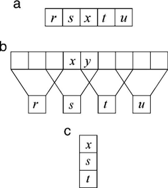
Three estimation tasks. (a) Estimation of missing image points. (b) Estimation of a high-resolution image from a low-resolution image. (c) Estimation of a missing color channel. Letters x and y represent values to be estimated; other letters represent observed values.

The most studied regularities in natural images involve single and pairwise statistics. For example, the intensities of randomly sampled points from a natural image have a probability distribution that is approximately Gaussian on a logarithmic intensity axis (Laughlin, 1981; Ruderman, Cronin, & Chiao, 1998), and the intensities of randomly sampled pairs of points have a covariance that declines smoothly as a function of the spatial separation between the points, in a fashion consistent with a Fourier amplitude spectrum that falls inversely with spatial frequency (Burton & Moorehead, 1987; Field, 1987; Ruderman & Bialek, 1994). Many other statistical regularities have been discovered by measuring pairwise statistics of image properties such as local orientation, color, spatial frequency, contrast, phase, and direction of motion (for reviews, see Geisler, 2008; Simoncelli & Olshausen, 2001). Much can be learned by measuring such pairwise statistics. For example, if the joint distribution of image features is Gaussian, then measuring the mean value of each feature and the covariance (a form of pairwise statistic) of the values for all pairings of features is sufficient to completely specify the joint distribution.

However, the joint distributions of many image features are not Gaussian and may not be completely described with pairwise statistics (Buccigrossi & Simoncelli, 1999; Daugman, 1989; Field, 1987; Zhu & Mumford, 1997), or it may be intractable to determine if they can be described by pairwise statistics. A useful strategy for characterizing statistical structure of natural images is to fit image data with some general class of generative model such as linear models that assume statistically independent but non-Gaussian sources (Bell & Sejnowski, 1997; Karklin & Lewicki, 2008; Olshausen & Field, 1997; van Hateren & van der Schaaf, 1998) or random Markov field models with filter kernels similar to those in the mammalian visual system (e.g., Portilla & Simoncelli, 2000; for reviews, see Simoncelli & Olshausen, 2001; Zhu, Shi, & Si, 2010). Alternatively, more complex joint distributions could be approximated with Gaussian mixtures (e.g., Maison & Vandendorpe, 1998). While these approaches have yielded much insight into the structure of natural images and neural encoding, they involve assumptions that may miss higher dimensional statistical structure (Lee, Pedersen, & Mumford, 2003).

In addition, weaker forms of assumed structure are sometimes implicit in normalization steps performed on each signal prior to the learning of their statistical structure. These normalization steps typically involve applying one of the following simple transformations to each training signal z (e.g., image patch): subtract the mean of the signal $(\mathbf{z}\prime =\mathbf{z}-\overline{\mathbf{z}})$, subtract the mean and then divide by the mean $(\mathbf{z}\prime =(\mathbf{z}-\overline{\mathbf{z}})/\overline{\mathbf{z}})$, subtract the mean and scale to a vector length of 1.0 $(\mathbf{z}\prime =(\mathbf{z}-\overline{\mathbf{z}})/\Vert \mathbf{z}-\overline{\mathbf{z}}\Vert )$, or subtract the mean and then multiply by a “whitening” matrix $({\mathbf{z}}^{\prime T}=\mathbf{W}{(\mathbf{z}-\overline{\mathbf{z}})}^T)$. Usually, these normalization steps are applied to simplify the mathematics or reduce the dimensionality of the estimation problem. The assumption is that the normalization preserves the important statistical structure. For example, it is plausible that the statistical structure of image patches is largely independent of their mean luminance, if they are represented as contrast signals by subtracting and dividing by the mean. Similarly, standard image processing algorithms for some of the point prediction tasks considered here implicitly assume that subtracting off the mean luminance of the observed signal preserves the relevant statistical structure. Thus, in both cases, the assumption is effectively that $p(\mathbf{z})=p(\mathbf{z}\prime )p(\overline{\mathbf{z}})$.

The most obvious strategy for characterizing statistical structure without making parametric assumptions is to directly estimate probability distributions by histogram binning. This strategy has proved useful for small numbers of dimensions (e.g., Geisler, Perry, Super, & Gallogly, 2001; Petrov & Zhaoping, 2003; Tkaèik, Prentice, Victor, & Balasubramanian, 2010). A more sophisticated strategy uses clustering techniques to search for the subspace (manifold) where natural image signals are most concentrated (Lee et al., 2003). While this strategy has provided valuable insight (e.g., the manifold is concentrated around edge-like features), the subspaces found are still relatively high dimensional and not precisely characterized.

An alternative strategy emphasized here is based on directly measuring moments along single dimensions, conditional on the values along other dimensions. Measuring conditional moments is a well-known approach for characterizing probability distributions (e.g., see statistics textbooks such as Fisz, 1967), and like directly estimating probability distributions, it is only practical for modest numbers of dimensions because of the amount of data required. Nonetheless, it has not been exploited for the current tasks and it has some unique advantages. First, univariate conditional distributions for local image properties are frequently unimodal and simple in shape, and thus, the first few moments capture much of the shape information. Second, estimating conditional moments only requires keeping a single running sum for each moment, making it practical to use essentially arbitrarily large numbers of training signals and hence to measure higher dimensional statistics with higher precision. Third, it is relatively straightforward to specify Bayes optimal estimators from conditional moments. Of central relevance here, the conditional first moment (conditional mean) is the Bayes optimal estimator when the cost function is the mean square error (i.e., the so-called MMSE estimator). Fourth, conditional moments can be combined allowing the approach to be extended to higher numbers of dimensions than would otherwise be practical.

The proposed conditional moment method is related to other non-parametric methods such as example-based methods of texture synthesis, where individual pixels are assigned the median (or mean) value of the conditional probability distribution estimated for the given surrounding context pixels (De Bonet, 1997; Efron & Leung, 1999).

Methods

Training and test stimuli

The image set consisted of 1049 images of outdoor scenes collected in the Austin area with a calibrated Nikon D700 camera (see Ing, Wilson, & Geisler, 2010 for the calibration procedure). The images contained no human-made objects and the exposure was carefully set for each image so as to minimize pixel response saturation and thresholding (clipping at high and low intensities). Each 4284 × 2844 14-bit raw Bayer image was interpolated to 14-bit RGB using the AHD method (Hirakawa & Parks, 2005). The RGB values were then scaled using the multipliers m_R = 2.214791, m_G = 1.0, and m_B = 1.193155 (which are determined by the camera make and model) to obtain a 16-bit RGB image. In the case of gray scale, YPbPr color space conversion was used (Gray = 0.299R + 0.587G + 0.114B). The dynamic range was increased by blacking out 2% of the darkest pixels and whiting out 1% of the brightest pixels. Blacking out pixels almost never occurred because in most images 2% of the pixels were already black. On the other hand, whiting out 1% of the brightest pixels has an effect because the image histograms have such long tails on the high end. For some measured statistics, the images were then converted to LMS cone space. Finally, the images were converted to linear 8-bit gray scale or 24-bit color. The images were randomly shuffled and then divided into two groups: 700 training images that were used to generate the tables and 349 test images. All pixels in the training images were used to estimate conditional moments, and thus, the number of training samples was on the order of 10¹⁰.

Conditional moments

The conditional moment approach is very straightforward. From the definition of conditional probability, an arbitrary joint probability density function over n dimensions can be written as a product of single dimensional conditional probability density functions:

$$p({\mathbf{x}}_n)={\displaystyle \prod _{i=1}^{n}p(x_i|{\mathbf{x}}_{i-1}),}$$ (1)

where x_i−1 = (x₁, …, x_i−1) and x₀ = ∅. Furthermore, the moments of a single dimensional probability distribution function defined over a finite interval (as in the case of image pixel values) are usually sufficient to uniquely specify the density function (e.g., Fisz, 1967). Thus, the full joint probability density function can be characterized by measuring the single dimensional conditional moments:

$$E(x_i^k|{\mathbf{x}}_{i-1})={\displaystyle \sum _{x_i}{x}_i^{k}p(x_i|{\mathbf{x}}_{i-1})},$$ (2)

where k is the moment (e.g., k = 1 gives the mean of the posterior probability distribution of x_i given x_i−1). As is standard, these moments can be estimated simply by summing the observed values of $x_i^k$ for each unique (or quantized) value of the vector x_i−1 and then dividing by the number of times the vector x_i−1 was observed:

$$E(x_i^k|{\mathbf{x}}_{i-1})\cong \frac{{\displaystyle \sum _{x_i\in \mathrm{\Omega }({\mathbf{x}}_{i-1})}{x}_i^k}}{N({\mathbf{x}}_{i-1})},$$ (3)

where Ω(x_i−1) is the set of observed values of x_i for the given value of the vector x_i−1, and N(x_i−1) is the number of those observed values.

We define the MMSE estimation function for x_i to be

$$f({\mathbf{x}}_{i-1})=E(x_i|{\mathbf{x}}_{i-1}),$$ (4)

which gives the Bayes optimal estimate of x_i when the goal is to minimize the mean squared error of the estimate from the true value (e.g., Bishop, 2006). The reliability of these estimates is given by

$$\rho ({\mathbf{x}}_{i-1})=1/\mathrm{VAR}(x_i|{\mathbf{x}}_{i-1}),$$ (5)

which is obtained from the first and second moments: $\mathrm{VAR}(x_i|{\mathbf{x}}_{i-1})=E(x_i^2|{\mathbf{x}}_{i-1})-E{(x_i|{\mathbf{x}}_{i-1})}^2$. The focus of most of this paper is on measuring and applying f(x_i−1) and ρ(x_i−1).

Given the number of training images, we were limited to directly measuring conditional moments for probability distributions with five or fewer dimensions. However, it is possible to obtain estimates based on even higher numbers of dimensions by combining estimates from different sets of conditional variables. For example, let ${\widehat{x}}_1$ be the estimate of x given one set of conditional variables, let ${\widehat{x}}_2$ be the estimate of x given a different set of conditional variables, and let ${\widehat{\rho }}_1$ and ${\widehat{\rho }}_2$ be their estimated reliabilities. If the estimates are Gaussian distributed and uncorrelated, then the optimal estimate given the combined conditional variables is

$$\widehat{x}={\widehat{x}}_1\gamma +{\widehat{x}}_2(1-\gamma ),$$ (6)

where $\gamma ={\widehat{\rho }}_1/({\widehat{\rho }}_1+{\widehat{\rho }}_2)$ is the relative reliability of the two estimates (e.g., Oruç, Maloney, & Landy, 2003; Yuille & Bulthoff, 1996). The more general combination rules for the case where the estimates are correlated are known (e.g., see Oruç et al., 2003); however, there are not enough training images to estimate these correlations. Nonetheless, applying Equation 6 can increase the accuracy of the estimates.

A more general way to combine the estimates that take into account relative reliability, and potentially other statistical structure, is to directly measure the MMSE function:

$$g({\widehat{x}}_1,{\widehat{x}}_2,\gamma )=E(x|{\widehat{x}}_1,{\widehat{x}}_2,\gamma ).$$ (7)

If sufficient training data are available, this function is guaranteed to perform at least as well as Equation 6.

It is important to note that none of these methods for combining the estimates are guaranteed to capture all of the additional statistical structure contained in the conditional moments of the combined variables. Nonetheless, they do make it practical to extend the conditional moment approach beyond five dimensions.

Results

Statistics

Conditional moments for three neighboring image points

To illustrate the conditional moment approach, consider first the conditional moments of an image point x given the two flanking values s and t (see Figure 1a). The direct method of measuring the kth moment, E(x^k|s, t), is simply to compute the running sum of the values of x^k for all possible values s, t, using every pixel in the 700 training images (see Equation 3). The result is a 256 × 256 table for each moment, where each table entry is for a particular pair of flanking values. These tables were estimated separately for horizontal and vertical flanking points; however, the tables did not differ systematically and hence were combined. This property held for the other cases described below, and hence, we show here only the combined tables.

Figures 2a–2d show tables of the first four moments, expressed as standard conditional central moments. Thus, the tables show the conditional mean, standard deviation, skew, and kurtosis of the center point for each pair of values of the flanking points. These tables have not been smoothed. Figure 2e shows the number of training samples that went into the estimates for each pair of flanking values. As can be seen, these natural image statistics are complex but very regular. The only trivial property of the tables is the symmetry about the diagonal, which simply says that s and t can swap locations without affecting the statistics. Some sense of what these tables represent can be gained from Figure 2f, which plots normalized histograms of x for the five pairs of flanking values indicated by the dots in Figures 2a–2d. These distributions are approximately unimodal and so are relatively well described by the first four moments.

Figure 2.

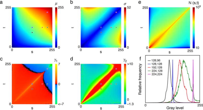
Conditional central moments for three neighboring image points. (a) The 1st moments are the means: μ = u₁. (b) The 2nd moments are plotted as the standard deviation: $\sigma =\sqrt{u_2}$. (c) The 3rd moments are plotted as the skewness: ${\gamma }_1=u_3/u_2^{3/2}$. (d) The 4th moments are plotted as the excess kurtosis: ${\gamma }_2=u_4/u_2^2-3$ (a Gaussian has an excess kurtosis of 0), where the central moments for each pair of values (s, t) were computed in the standard way: $u_1=n^{-1}{\displaystyle \sum x},u_2=n^{-1}{\displaystyle \sum {(x-u_1)}^2},u_3=n^{-1}{\displaystyle \sum {(x-u_1)}^3,u_4=n^{-1}{\displaystyle \sum {(x-u_1)}^4}}$ (see Kenny & Keeping, 1951; Papoulis, 1984). (e) Number of training samples for each value of s, t. (f) Conditional distributions for the five sample pairs of (s, t) values indicated by the dots in (a)–(d). The plots have not been smoothed.

The table of conditional first moments in Figure 2a gives the Bayes optimal MMSE estimate of x given a flanking pair of points. The table of conditional second moments can be used to combine separate MMSE estimates (e.g., estimates based on horizontal and vertical flanking points; see later). Maximum a posteriori (MAP) estimates (or estimates based on other cost functions) should be possible using the four moments to estimate the parameters of a suitable family of unimodal density functions. However, the focus in the remainder of this paper is on MMSE estimates.

Estimation of missing or occluded image points

Consider first the case of estimating x from just the two nearest flanking values (s, t). The MMSE estimate function f(s, t) is given by the table in Figure 2a. If the joint probability distribution p(x, s, t) were Gaussian, then (given two obvious constraints that apply in our case: when s = t, the optimal estimate is s, and symmetry about the diagonal) the optimal estimate would be the average of the two flanking values: f(s, t) = (s + t)/2 (see Appendix A). Similarly, if the joint probability distribution p(x, s, t) is Gaussian on log axes, then the optimal estimate would be the geometric average of the two flanking values: $f(s,t)=\sqrt{st}$. These are useful references against which to compare the measured table.

The plot in Figure 3b shows the difference between the measured table and the table predicted if the joint distribution were Gaussian (the prediction of linear regression). As can be seen, there are systematic but complex differences between the directly measured function and the Gaussian prediction. The black pixels show cases where the optimal estimate is equal to the average of the flanking pixel values. The warm-colored pixels indicate cases where the estimate is above the average of the flanking pixels and the cool-colored pixels where the estimate is below the average. Examining where differences from the Gaussian prediction occur in representative natural images suggests that they tend to be associated with well-defined contours.

Figure 3.

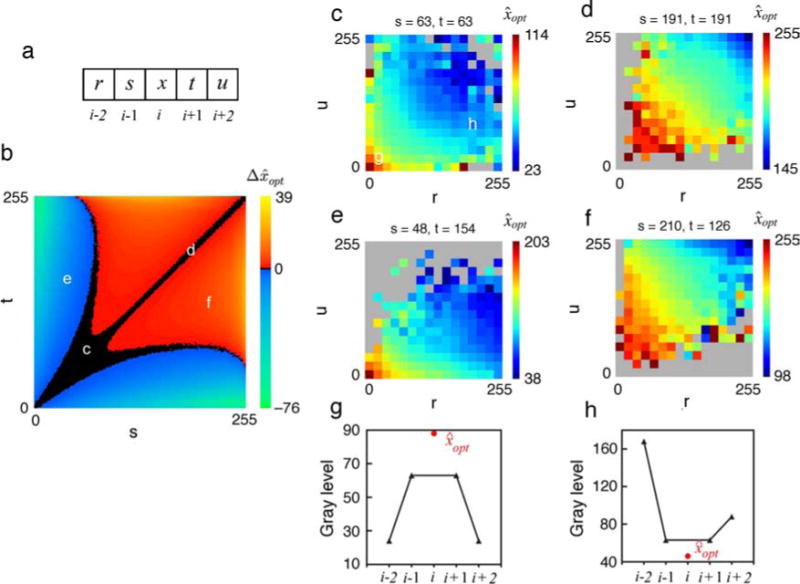
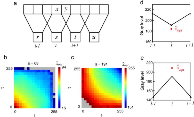
Estimation of a missing or occluded point. (a) In the case of third-order statistics, the aim is to predict x from (s, t). In the case of fifth-order statistics, the aim is to predict x from (r, s, t, u). (b) Optimal estimation of x given (s, t). The color map shows the difference between the optimal estimate and average of s and t, which corresponds to the optimal estimate assuming a Gaussian joint distribution. (c–f) Optimal estimation of x from (r, s, t, u), for the specific values of (s, t) indicated by the white letters in (b); (c) (63, 63), (d) (191, 191), (e) (48, 154), (f) (210, 126). Each plot gives the optimal estimate as a function of the further flanking values r and u. Gray indicates no data. (g, h) Examples of specific point predictions for the two quantile bins labeled in (c). The black triangles show the observed values (r, s, t, u); the red circle shows the optimal prediction.

Importantly, there are no obvious forms of invariance in Figure 3b (or Figure 2a), except for the expected diagonal symmetry: f(s, t) = f(t, s). In other words, the optimal estimates depend on the specific absolute values of s and t, not only on their relative values. The lack of obvious invariance in Figure 3b shows that less direct methods of measuring the image statistics could have missed important structure. For example, suppose each signal were normalized by subtracting the mean of s and t before measuring the conditional first moments, and then the mean was added back in to create a table like Figure 2a. If this procedure did not miss any information, then the difference values plotted in Figure 3b would be constant along every line parallel to the diagonal (see Appendix A). In fact, most interpolation methods (e.g., linear, cubic, and spline methods) ignore the mean signal value and consider only the difference values. Similarly, if normalizing each signal by subtracting and dividing by the mean of s and t before measuring the conditional first moments did not lose information, then the difference values in Figure 3b would be constant along any line passing though the origin (see Appendix A). In other words, these common preprocessing steps would have led us to miss some of the statistical structure shown in Figure 3b. Similar conclusions are reached if the log Gaussian prediction is used as the reference, suggesting that the complex structure and the lack of invariance are not due to the non-Gaussian shape of the marginal distribution of intensity values. As a further test, we quantized the 14-bit raw images into 8-bit images having an exactly Gaussian histogram, and then ran the above analyses. The resulting plots are qualitatively similar to those in Figure 3b.

Now consider the case of estimating x from all four neighboring values (r, s, t, u). In this case, the goal is to measure the MMSE estimation function:

$$f(r,s,t,u)=E(x|r,s,t,u).$$ (8)

To facilitate measurement and visualization of this four-dimensional function, it is useful to measure and plot separate two-dimensional tables for each pair of values (s, t). In other words, we measure 2¹⁶ tables of the form f_s,t(r, u). This set of two-dimensional tables constitutes the full four-dimensional table.

The direct method of computing the mean of x for all possible flanking point values is not practical given the amount of image data we had available. One way to proceed is to lower the resolution of the table for the furthest flanking points. Reducing the resolution is justifiable for two reasons: (i) the furthest flanking points should generally have less predictive power, and (ii) reducing resolution is equivalent to assuming a smoothness constraint, which is plausible given the smoothness of the third-order statistics (plot in Figure 2a). We quantized the values of r and u into 16 bins each:

$$f_{s,t}(r,u)\cong f_{s,t}(q(r),q(u)),$$ (9)

where q(·) is a quantization function that maps the values of r and u into 16 integer values between 0 and 255.

The plots in Figures 3d–3f are representative examples of tables for the different values of (s, t) corresponding to the white letters in Figure 3b. As in Figure 2a, the color indicates the optimal estimate. (In the plot, gray indicates values of (r, s, t, u) that did not occur in the training set.) Again, the statistical structure is complex but relatively smooth and systematic. Consider the tables for values of (s, t) that are along the diagonal (s = t). When the values of r and u are below s and t, then (r, s, t, u) is consistent with a convex intensity profile and the estimate is above the average of s and t (see Figure 3g). On the other hand, when the values of r and u exceed s and t, then (r, s, t, u) is consistent with a concave intensity profile and the estimate is below the average of s and t (see Figure 3h). Similar behavior is seen in the tables for values of (s, t) that are not along the diagonal, but the tables are less symmetric. These are intuitive patterns of behavior, but again, there are no obvious forms of invariance except for the diagonal symmetry when s = t.

As mentioned earlier, the estimation functions obtained by analyzing horizontal and vertical flanking points do not differ systematically, and thus, in each case the horizontal and vertical data were combined to obtain a single estimation function, which can be applied in either direction. However, when this function is applied in both the horizontal and vertical directions, for the same image point, somewhat different estimates are often obtained. In other words, there is additional information available in the two estimates.

It is possible to characterize some of this additional information by measuring the relative reliability of the two estimates, which determines how much weight each should be given in the combined estimate. The blue curve in Figure 4a plots the distribution of relative reliability for the missing image point (interpolation) task when the two estimates are based on the horizontal and vertical values of (r, s, t, u). There is considerable variation in the relative reliability, suggesting that this measure contains useful information. This large variation may be due to the structure of intensity gradients in natural images. As shown in Figure 2b, estimates based on image points that are near equal are more reliable than estimates based on image points that are less equal. However, image points that are relatively parallel to the local intensity gradient are closer to equal than image points that are relatively perpendicular to the local intensity gradient. In the performance demonstrations below, we combine horizontal and vertical estimates ( ${\widehat{x}}_{\mathrm{H}}$ and ${\widehat{x}}_{\mathrm{V}}$) using relative reliability (see Equation 6 in the Methods section).

Figure 4.

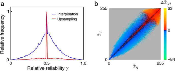
Reliability and recursive estimation. (a) Relative frequency of the relative reliability of the two estimates based on values in the horizontal and vertical directions for the task of estimating the missing or occluded image point (blue curve) and estimating a higher resolution image point (red curve). (b) Recursive estimation function for upsampling. The horizontal axis gives the optimal estimate of x given the observed values in the horizontal direction in the image, and the vertical axis gives the optimal estimate of x given the observed values in the vertical direction. The color scale gives the estimate of x given the estimates in the two directions minus the average of the two optimal estimates, for a relative reliability of 0.5. Gray indicates no data.

Estimation of a high-resolution image from a low-resolution image

The task of upsampling from a low-resolution to a high-resolution image is illustrated in Figure 5a. Upsampling involves both interpolation and compensation for spatial filtering. In general, a low-resolution image can be conceptualized as being obtained from a higher resolution image by the operation of low-pass spatial filtering followed by downsampling. For example, a well-focused camera image (or a foveal cone image) can be regarded as a higher resolution image that has been filtered by a small amount of optical blur plus summation over the area of the sensor element, followed by downsampling at the sensor element locations. As illustrated in Figure 5a, we consider here the case where the filtering operation has an odd kernel so that each low-resolution image point is centered on a high-resolution image point. The case for an even kernel is similar but differs in certain details (it is somewhat simpler).

Figure 5.

Estimation of a high-resolution image from a low-resolution image. (a) Fourth-order statistics are used to predict x from (r, s, t) and fifth-order statistics are used to predict y from (r, s, t, u). (b, c) Optimal estimation of x given (r, s, t) for two values of s. The color indicates the optimal estimate of x. Gray indicates no data. (d, e) Examples of specific point prediction for two bins in (c). The black triangles are specific values (r, s, t); the red circles are the optimal estimates.

As shown in Figure 5a, different statistics were used for estimating points like x that are aligned with low-resolution points and those like y that are centered between low-resolution points. Following similar logic as before, the Bayes optimal estimate of x is given by E(x|r, s, t) and the optimal estimate of y is given by E(y|r, s, t, u), and thus, our aim is to measure the functions f_s(r, t) for the aligned points (x) and the functions f_s,t(r, u) for the between points (y). To measure these functions, we first filtered all of the calibrated images with a 3 × 3 Gaussian kernel and then downsampled them by a factor of two in each direction to obtain a set of low-resolution images together with their known higher resolution “ground-truth” images. As before, we quantized the more distant image points, and thus, we measured f_s(q(r), q(t)) and f_s,t(q(r), q(u)), where q(·) is a quantization function.

Examples of the tables measured for the aligned points (x) are shown in Figures 5b and 5c. The plots show the optimal estimate of x. As can be seen, if the values of r and t are greater than s, then the optimal estimate of x is less than s (see Figure 5d), and vice versa if the values of r and t are less than s (see Figure 5e). The tables measured for the between points (y) are similar to those in Figures 3c–3f. The tables plotted in Figure 5 are intuitively reasonable and reflect both the structure of the natural images and the effect of the blur kernel.

The relative reliability for the horizontal and vertical estimates of the aligned points (x) is shown by the red curve in Figure 4a. The relative reliability is concentrated around 0.5, suggesting that this measure contains less useful information than in the case of the missing image point task. Indeed, we found that more useful information is contained in the recursive conditional first moments (see Equation 7 in the Methods section). Figure 4b plots the estimate of x given ${\widehat{x}}_{\mathrm{H}}$ and ${\widehat{x}}_{\mathrm{V}}$ minus the average of the two estimates, for a relative reliability (γ) of 0.5. Again, the statistics are complex but regular. If the estimates nearly agree, then the best estimate is near the average of the two estimates. If the estimates do not agree, then the best estimate is higher than the average when the average is big but lower than the average when the average is small.

Estimation of a missing color channel

The task of estimating a missing color channel is illustrated in Figure 1c. Recall that in this task we ignore spatial information. We consider the task of estimating each color channel given the other two. We do this for two cases, one where the three channels are the R, G, and B sensors in the camera, and the other where the three channels are the L, M, and S cones in the human retina. In other words, we measured the following statistics: E(R|G, B), E(G|R, B), E(B|R, G), E(L|M, S), E(M|L, S), and E(S|L, M). Recall that these first conditional moments are the Bayes optimal estimates when the goal is to minimize the mean squared error.

Figure 6 plots the estimates for each class of sensor. Once again, the statistics are complex but regular, and there are no obvious forms of invariance. In other words, the estimates of a color channel value depend on the specific absolute values of the other channels.

Figure 6.

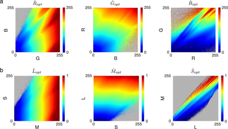
Estimation of a missing color channel. Plots show the optimal estimate of the missing color value given the observed color values on the horizontal and vertical axes. (a) Estimation of missing R, G, or B camera responses. (b) Estimation of missing L, M, or S cone responses. Gray indicates no data.

Performance

The measurements in Figures 2–6 reveal complex statistical structure in natural grayscale and color images. These statistics are of interest in their own right, but an obvious question is what their implications might be for vision and image processing. Perhaps the most fundamental questions are: How useful would knowledge of these statistics be to a visual system? And, does the human visual system use this knowledge? The conditional first moments in Figures 2–6 give the Bayes optimal (MMSE) estimates for the specific tasks shown in Figure 1. Thus, to address these questions, we could compare optimal performance on these tasks with that of other simpler estimators, and we could also potentially compare ideal and human performance in the first two tasks (i.e., subjects could make estimates based on a short row or column of natural image pixels). While this is doable and potentially useful, we show here predictions for the third task and for the two-dimensional versions of the first two tasks, where multiple estimates are combined using the measured recursive conditional moments. Although we cannot guarantee optimal performance on the two-dimensional tasks, they are closer to the normal image processing tasks carried out in biological and artificial vision systems. All comparisons were carried out on a separate random sample of test images.

Estimation of missing or occluded image points

For each pixel in each test image, we estimated its value by applying the MMSE estimation function f(r, s, t, u) in both directions and combining the two estimates using the measured relative reliability. This is what we call the biprior estimator. We also estimated the value of each pixel using the standard bilinear estimator. Estimation accuracy is quantified as the peak signal-to-noise ratio, PSNR = 10log(255²/MSE), where MSE is the mean squared error between the estimated and true values. Thus, a 50% decrease in MSE corresponds to a 3-db increase in PSNR. Figure 7a plots for each test image the difference in the PSNR of the two estimators as a function of the PSNR of the bilinear estimator. All blue points above zero indicate images for which the biprior method was more accurate. In general, the biprior method performs better. The increases in performance are substantial (3.7 db on average) and demonstrate the potential value of the natural image statistics in estimating missing or occluded points.

Figure 7.

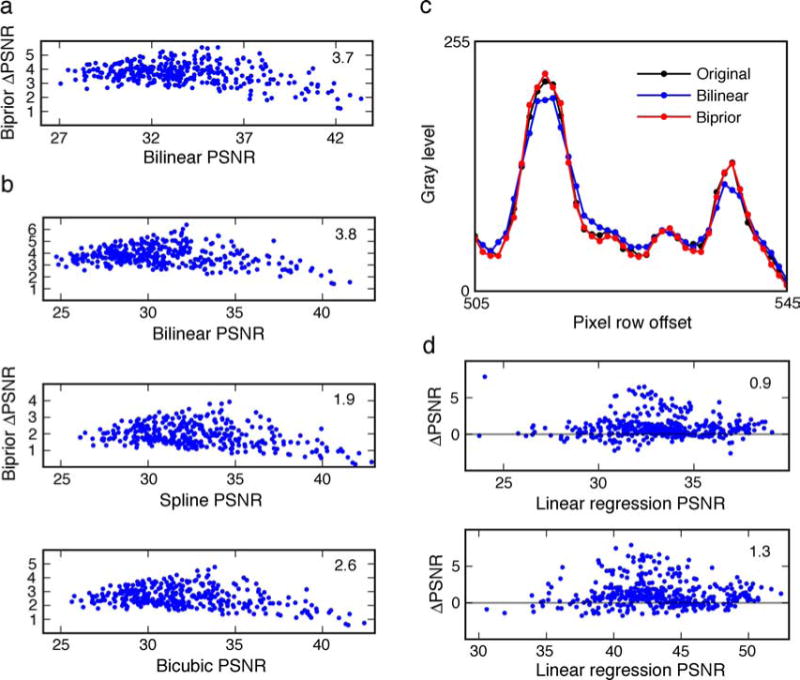
Performance in three estimation tasks. (a) Estimation of missing or occluded image points. The difference in peak signal-to-noise ratio (PSNR) between the biprior and bilinear estimators for the 349 test images, as a function of the PSNR of the bilinear estimator, is plotted. Each point represents a test image; points above zero indicate better performance for the biprior estimator. The average increase in PSNR across all test images is 3.7 db. (b) The difference in PSNR for upsampling of the 349 test images as a function of the PSNR of the method is indicated on the horizontal axis. (c) Comparison of bilinear and biprior interpolation along a segment of scan line from a test image. (Note that every other interpolated scan line, like this one, contains no original image pixels.) (d) Difference in PSNR between optimal estimator and linear estimator (linear regression) as a function of the PSNR for the linear estimator. The upper plot is for RGB images and the lower plot for LMS images. The values of PSNR are computed in the CIE L*a*b* color space.

If the biprior estimate is based on only one direction, then the increase in performance over bilinear is 1.0 db on average, and if the two estimates are simply averaged (given equal weight), then the average increase in performance over bilinear is 3.2 db. Thus, all components of the biprior estimator make a substantial contribution to performance. If only the two neighboring pixel values are used (i.e., applying f(s, t) in both directions and combining with relative reliability), the increase in performance over bilinear is 0.9 dB. This shows that the complex statistical structure shown in Figures 2 and 3a is useful, but it also shows that the additional flanking pixels make a substantial contribution to performance.

We also explored a number of related methods to determine if significant improvements in performance were possible. First, we applied exactly the same method for the diagonal directions rather than cardinal directions and found performance to be worse than even the simple bilinear estimator. Further, combining the diagonal estimates with the cardinal estimates did not improve the performance of the biprior estimator. This suggests that the pixels closest to the missing pixel carry most of the useful information. Next, we explored one- and two-dimensional kernels obtained with principal component analysis (PCA). The one-dimensional kernels were obtained for the 6 pixels on the two sides of the missing pixel in the horizontal or vertical direction. The two-dimensional kernels were obtained for the 24 surrounding pixels in a 5 × 5 block. We then applied the current conditional moment method for different choices of four PCA kernels. In other words, for each test stimulus, we applied the four kernels and used the resulting four values as the context variables (r, s, t, u). None of these performed well. Next, we explored one- and two-dimensional kernels obtained using a recent method (accuracy maximization analysis) that finds kernels that are optimized for specific identification and estimation tasks (Geisler, Najemnik, & Ing, 2009). In the one-dimensional case, we found that the AMA kernels were essentially equivalent to (covered approximately the same subspace as) the four kernels corresponding to the separate 4 pixels in the horizontal or vertical direction and did not produce a significant improvement in performance. In the two-dimensional case, we found that the four AMA kernels performed much better than the estimates based on only one direction but did not perform better than the combined vertical and horizontal estimates. Finally, we tried combining the horizontal and vertical estimates with the full recursive table (Equation 7) and found only a very slight increase (less than 1%) in performance over using Equation 6. While none of these analyses is definitive, together they suggest that the biprior estimator makes near optimal use of the local image structure in natural images for the 2D missing image point task.

Estimation of a high-resolution image from a low-resolution image

For measuring the accuracy of the upsampling methods, the test images were blurred by a 3 × 3 Gaussian kernel, downsampled by a factor of two in each direction, and then upsampled using one of four methods: biprior, bilinear, spline, and bicubic upsampling. Bilinear upsampling uses linear interpolation of the two nearest neighbors, applied in both directions. Spline upsampling uses cubic interpolation of the four nearest neighbors (along a line) in both directions. Bicubic upsampling uses full cubic interpolation of the 16 (4 × 4) nearest neighbors. Biprior upsampling used tables for x points having 256 levels (8 bits) each for r, s, and t. The horizontal and vertical estimates for the x points were then combined using the recursive table (see Equation 7 and Figure 4b). These estimated x points were then used as the four flanking points to estimate the y points. One final point in each 3 × 3 block (a z point not shown) was estimated by combining vertical and horizontal estimates from the flanking estimated y points, using the recursive table. The results are shown in Figure 7b. The biprior estimator performs substantially better than the standard methods on all the test images, demonstrating the potential value of the measured natural image statistics in decoding photoreceptor (or ganglion cell) responses. As in the case of estimating the missing point, all components of the biprior estimator make a substantial contribution to performance. However, unlike missing point estimation, using only the reliability to combine horizontal and vertical estimates (Equation 6) did not work as well as using the recursive table, presumably because of the smaller variation in relative reliability (red curve in Figure 4a).

A closer look at the differences between bilinear and biprior estimates is shown in Figure 7c, which plots the bilinear (blue) and biprior (red) estimates against the original image points (black) for a typical segment of a scan line from a test image.

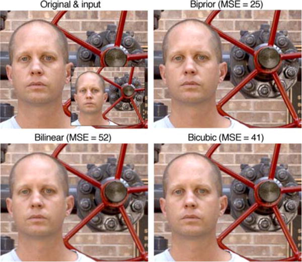
Figures 8 and 9 compare the original and the downsampled input images with the upsampled images obtained using the biprior, bilinear, and bicubic methods. In addition to largely maintaining the original contrast, the biprior method does a better job of restoring detail. Similar behavior is seen with all the images we have inspected from the set of test images; indeed, the improvement in MSE for these images relative to bilinear (53% and 52%, respectively) is slightly less than the median improvement of 58%. The upsampling of these color images was obtained by applying the same estimator to each color channel. The relative improvement in MSE of the biprior estimator for these color images is only very slightly less (about 1%) than for the grayscale images on which the image statistics were learned. This demonstrates the robustness of the image statistics. Figure 9 also demonstrates the robustness of the image statistics in that the training set contained no human-made objects or human faces.

Figure 8.

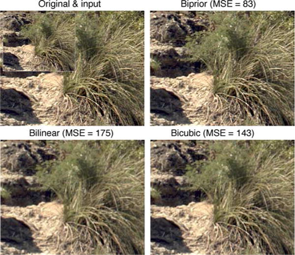
Comparison of upsampling based on natural scene statistics (biprior method) with standard methods based on bilinear and bicubic interpolation. This is a representative example from the 349 test images; the reduction in mean squared error for biprior relative to bilinear is 53%, whereas the median reduction is 58%. The large image in the upper left panel is the original image and the inset is the downsampled input image.

Figure 9.

Comparison of upsampling based on natural scene statistics (biprior method) with standard methods based on bilinear and bicubic interpolation. Images of faces and human-made objects were not in the training set of images. Thus, this example demonstrates the robustness of the statistics.

Estimation of a missing color channel

To test the performance accuracy of the Bayes optimal estimators for missing color channels, we separately removed each channel and then estimated the value of that channel at each pixel location in each test image. We quantified the estimation accuracy by the mean squared error between the estimated and original colors in the CIE L*a*b* uniform color space. The average increase in PSNR of the optimal estimate over that of linear regression is as follows for each color channel: (R, G, B) = (1.2 db, 0.59 db, 0.93 db) and (L, M, S) = (1.3 db, 0.91 db, 2.3 db). Note that linear regression incorporates all the pairwise correlations between the color channels (i.e., the full covariance matrix). Also, note that there are many locations in the color spaces of Figure 6 for which there is no data (the gray areas), and thus, one might wonder if performance would be better if the spaces were filled in better. In fact, this is not an issue. For the random set of test images, there were very few occasions when an empty location was encountered (less than 1 pixel per two images).

Estimation accuracy was not equally good for each color channel in an image. The percentage of images where each channel was easiest to estimate are as follows: (R, G, B) = (62%, 26%, 12%) and (L, M, S) = (78%, 22%, 0%). Figure 7d plots the difference in PSNR between the optimal estimator and the linear estimator (linear regression) as a function of the PSNR for the linear estimator, for the channel that was easiest to estimate. (Usually, the channel that was easiest to estimate was the same for the optimal and linear estimators, but in a small percentage of cases, the best channel was different.) The upper panel plots accuracy for a missing R, G, or B channel and the lower panel for a missing L, M, or S channel. Points above the horizontal line indicate images where the optimal estimate was more accurate than the linear regression estimate.

Several randomly selected examples are shown in Figure 10. The first column shows the original image. The second column shows the image after a color channel has been removed (the channel values set to zero). The third column shows the result of applying the optimal estimator. Finally, the fourth column shows the result of the linear regression estimator. Although the color is not accurately reproduced, it is nonetheless surprising how natural the estimated images in the third column look, in the sense that one would be hard-pressed to say that a color channel had been estimated without seeing the original. The estimates based on linear regression are also impressive, but they tend to look either too uniform or too purple/violet in color. For example, notice the lack of browns and tans in the bottom three rows, the purple tinted sky in the second row, and the pink tinted leaves in the first row. Thus, it appears that the statistics in Figure 6 capture substantial color redundancy in natural outdoor images that is not captured by linear regression (e.g., Gaussian models).

Figure 10.

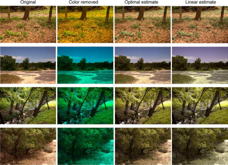
Estimation of a missing color channel. In the first row, the B channel is estimated. In the other rows, the R channel is estimated. In row 3, the linear estimate is more accurate than the optimal estimate. Interestingly, the optimal estimate appears more “natural” in color, which was generally true.

Discussion

A direct conditional moment approach was used to measure joint statistics of neighboring image points in calibrated grayscale and color natural images. Specifically, optimal (MMSE) estimators were measured for the tasks of estimating missing image points, estimating a higher resolution image from a lower resolution image (super resolution), and estimating a missing color channel. In the different cases, the measured estimators are functions of two, three, or four neighboring image points. In general, we find that the estimation functions are complex but also relatively smooth and regular (see Figures 2–6). Importantly, the MMSE functions have no obvious forms of invariance, except for an expected diagonal symmetry. The lack of invariance implies that the various simplifying assumptions of invariance that are typical in less direct measurement methods probably miss important statistical structure in natural images. This conclusion is clearest for the invariance assumptions implicit in the preprocessing transformations often applied to training signals (e.g., subtracting off the local mean or subtracting and scaling by the local mean), but it probably holds for a number of other invariance assumptions as well.

To begin exploring the implications of the measured statistics, we compared the performance of the Bayesian MMSE estimators with standard methods. We find that against objective ground truth, the MMSE estimators based on natural image statistics substantially outperform these standard methods, suggesting that the measured statistics contain much useful information. Thus, our results have potentially important implications for understanding visual systems and for image processing. Specifically, given the demonstrated usefulness of the statistics, it seems likely that these statistics have been incorporated, at least partially, into biological vision systems, either through evolution or through learning over the life span. Furthermore, because the measured statistics are so rich and regular, they make many predictions that should be testable in psychophysical experiments.

For example, the task of estimating missing image points could be translated into psychophysical experiments using a paradigm similar to that of Kersten (1987), where observers are asked to estimate the grayscale value at the missing image points. The natural image statistics measured in Figures 2 and 3 make many strong predictions. Whenever the values of r and u are below s and t in r, s, t, u space (see Figure 3), observers are predicted to estimate gray levels above the average of s and t, and the opposite when r and u are above s and t. Further, the uncertainty in the observers’ estimates (e.g., psychometric function slopes) should be greater in those parts of the space where the standard deviations of the conditional moment distributions are greater (see Figure 2b).

Similarly, the task of estimating a higher resolution image from a lower resolution image could be translated into psychophysical experiments where observers are asked to compare altered foveal image patches with unaltered patches presented in the periphery. Specifically, if the visual system exploits the natural image statistics in Figures 4b and 5b, then a foveal patch that corresponds to the optimal upsampled estimate from the half-resolution version of the patch should be the best perceptual match to the (unaltered) patch presented at the appropriate eccentricity. Such predictions could be tested by varying the foveal patch around the optimal estimate.

The task of estimating the missing color channel is probably not so directly translatable into psychophysical experiments. However, the joint prior probability distribution represented by the conditional moments in Figure 6, and the other moments not shown, could play a role in understanding how photoreceptor responses are decoded. For example, Brainard et al. (2008) have shown that estimates of color names from the stimulation of single cones (Hofer, Singer, & Williams, 2005) is moderately predictable using a Bayesian ideal estimator that takes into account the spatial arrangement of the subjects’ L, M, and S cones, as well as the prior probability distribution over natural images. They assumed that the prior is Gaussian and separable over space and color. The present statistics show that the prior over color is not Gaussian and that color estimation is more accurate if the joint statistics are taken into account. Thus, the present results may lead to somewhat different predictions for estimation experiments like those of Hofer et al. (2005).

The optimal estimators for the present tasks depend on both the statistical properties of the images in the training set as well as the spatial filtering and noise characteristics associated with the imaging system capturing the images. This suggests that there may be many different scientific and practical applications for the conditional moment approach described here. For example, the statistics of medical images, microscopic images, satellite images, and diagnostic images in manufacturing and safety inspection are likely to be different in detail from the natural images considered here. Measurement of conditional moments for these other classes of image could potentially lead to a better understanding of their statistical structure and to substantially improved resolution, interpolation, and/or noise suppression. In general, the conditional moment approach may be applicable and useful whenever there is a sufficiently large set of training images. The approach could also be applied to natural signals other than natural images.

An advantage of the simple conditional moment approach is that it can be applied easily to arbitrarily large training sets, allowing relatively precise measurements of joint statistics. The number of training signals here was on the order of 10¹⁰ and much larger training sets are possible. However, measuring the conditional moments is not feasible once the signal dimensionality becomes sufficiently high (although the dimensionality can be extended somewhat by measuring recursive conditional moments that take into account reliability; see Equations 6 and 7 in the Methods section). In high dimensions, parametric models are the most viable approach. Nonetheless, even when the dimensionality is high, conditional moments measured in lower dimensions may be useful for constraining parameters and testing the assumed forms of invariance in the parametric models. An important two-dimensional example of this was the discovery that the unsigned magnitudes of nearby orthogonal wavelet values are positively correlated, even when their signed values are uncorrelated (Buccigrossi & Simoncelli, 1999).

The conditional moment approach works very well for the estimation tasks described here because these tasks are inherently low dimensional. The missing color task is exactly three-dimensional, and hence, there is sufficient data to accurately determine the full MMSE estimators. For the two-dimensional missing point task, we demonstrated that the relevant information is highly concentrated in the neighboring 4 pixels in the horizontal and vertical directions. Our analyses are not definitive but nonetheless suggest that substantially better performance cannot be obtained by moving to higher dimensions. Similar conclusions are likely for the two-dimensional upsampling (super resolution) task. However, for tasks that are inherently higher dimensional (e.g., that involve integrating information over larger spatial areas), the conditional moment approach will be less useful.

With respect to practical application, it is worth noting that the estimators described here consist of fixed tables and hence can be applied by a simple lookup (albeit with substantial memory requirements for the tables). (Of course, parametric models in similarly low-dimensional spaces could also be tabled.) The estimation functions also appear to be relatively smooth, so it may be possible to find simple formulas that provide close approximation.

Could the conditional moment approach be useful for practical image processing tasks? Our goal here is to characterize image statistics rather than develop image processing algorithms. Nonetheless, we have made some preliminary comparisons with existing algorithms. Figure 11 shows a comparison with various recent super resolution (upsampling) algorithms (Fattal, 2007; Freeman et al., 2002; Glasner et al., 2009; and a commercial algorithm, Perfect Resize 7.0), rank ordered by the mean squared error from the original image (in parentheses). The upsampling is by a factor of 4 and only a part of the image is shown, in order to make the differences between the algorithms more visible. Although the biprior algorithm has the lowest MSE, the smoothness of the pupil boundary is better captured by some of the other algorithms. On the other hand, the texture of the hat and the inside of the iris is better captured by the biprior algorithm. In addition, some of the other algorithms are computationally intensive; the Freeman algorithm is reported to take over 30 min to produce a 0.25-MB (512 × 512) image, the Glasner algorithm 90 s, and the Fattal algorithm 6 s. On the other hand, the biprior algorithm produces a 12-MB (4000 × 3000) image in about 0.1 s. Thus, there may be upsampling applications where the conditional moment approach will have practical value.

Figure 11.

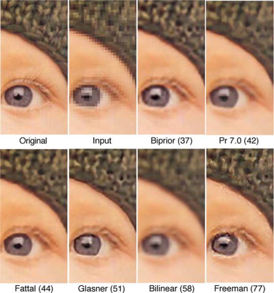
Comparison of different upsampling (super resolution) algorithms. The original image was 512 × 512 and input was 128 × 128. The numbers in parentheses are MSE from the original image. The original and input images were provided by R. Fattal (http://www.cs.huji.ac.il/~raananf/projects/upsampling/results.html) and the upsampled images for the Fattal, Freeman, and Glasner algorithms were provided by M. Irani (http://www.wisdom.weizmann.ac.il/~vision/SingleImageSR.html). Some appreciation for the sources of some of the distortions seen in the upsampled images can be obtained by inspecting the input image.

To get some idea of whether the conditional moment approach might be useful for other image processing tasks, we put together a few unoptimized test algorithms. Their performance suggests that the conditional moment approach is promising or, at least, may provide useful insight in developing practical algorithms. A first pass at interpolation of Bayer images (demosaicing digital camera images) gave mean squared error (MSE) performance better than the AHD algorithm (e.g., see Hirakawa & Parks, 2005), a common current standard, and comparable to more recent algorithms (Li et al., 2008; also see Mairal, Elad, & Sapiro, 2008). A first pass at denoising (for additive Gaussian noise) gave MSE performance equal to adaptive Weiner filtering (MatLab wiener2; Lim, 1990). A first pass at lossless compression gave compression ratios in between those of PNG and JPEG-LS, the best current standards (for references and discussion, see Santa-Cruz, Ebrahimi, Askelof, Larsson, & Christopouos, 2000). Another potential application is in color reproduction. To enhance color reproduction, video displays have begun using a 4th color channel (e.g., the Sharp Quattron). As in our third task, the conditional moment method could be used to find the Bayes optimal estimate of the 4th (yellow) channel values given the RGB values and hence potentially improve the quality (and accuracy) of standard RGB imagery displayed on a 4-channel device.

Another future direction is to investigate the underlying causes of the complex statistical regularities reported here. For the first two tasks, inspections of the image locations where deviations from the linear prediction are greatest suggest (not surprisingly) that the causes are at least in part related to the properties of well-defined edges (see Figure 7c) but much remains to be done.

The full set of natural images and many super-resolution examples are available at http://www.cps.utexas.edu/natural_scenes.

Appendix A

Gaussian and log Gaussian models for optimal interpolation between two points

Here, we derive the optimal estimate of the central point in optimal interpolation under the assumption that the underlying distributions are Gaussian and log Gaussian. A conditional Gaussian distribution p(x_a|x_b) has a mean value that is a linear function of x_b and a covariance that is independent of the value of x_b. Therefore, in the case of interpolation between two points, the optimal estimate is given by

$${\widehat{x}}_{\text{opt}}=w_{1}s+w_{2}t+w_0.$$ (A1)

However, there are two empirical constraints that also hold in our case. First, when s = t, we always find (in agreement with intuition) that

$${\widehat{x}}_{\text{opt}}=s=t,$$ (A2)

which implies that w₀ = 0. Second, we observe (in agreement with intuition) symmetry about the diagonal (see Figure 1b), which requires that

$$w_1=w_2,$$ (A3)

which implies that $w_1=w_2=\frac{1}{2}$ and hence ${\widehat{x}}_{\text{opt}}=\frac{s+t}{2}$. The same relations hold for a log Gaussian distribution, except $\log {\widehat{x}}_{\text{opt}}=\frac{\log s+\log t}{2}$ or ${\widehat{x}}_{\text{opt}}=\sqrt{st}$ (the geometric average).

Implications of standard transformations of training signals

Two of the standard preprocessing steps in measuring natural signal statistics are: (a) subtract off the mean of each training signal to obtain a collection of zero mean signals or (b) subtract off the mean and then divide by the mean to obtain a collection of normalized zero mean signals (e.g., signed contrast signals). Even when these steps are not carried out explicitly, they are frequently an implicit component of statistical analyses. These steps are intuitively sensible because they remove seemingly irrelevant information when the goal is to characterize the statistics of signal shape. However, they correspond to invariance assumptions that can lead to missed information. To see this, consider the case of measuring the expected value function for the central pixel given the two neighboring pixel values: f(s, t) = E(x|s, t) (see Figures 3a and 3b).

Transforming training signals to zero mean

Let (s_i, x_i, t_i) be an arbitrary original training signal and let m_i be the local mean (s_i + t_i)/2 that is subtracted off. The transformed values of s_i, x_i, and t_i are given by

$$s_i^{\prime }=s_i-m_i,x_i^{\prime }=x_i-m_i,t_i^{\prime }=t_i-m_i.$$ (A4)

In this case, for all possible learning algorithms:

$$\text{if}(s_i^{\prime },t_i^{\prime })=(s_j^{\prime },t_j^{\prime }),\text{then}E(x^{\prime }|s_i^{\prime },t_i^{\prime })=E(x^{\prime }|s_j^{\prime },t_j^{\prime }).$$ (A5)

What is the set of (s_j, t_j) for which $(s_i^{\prime },t_i^{\prime })=(s_j^{\prime },t_j^{\prime })$? For any given (s_i, t_i), the (s_j, t_j) must satisfy the following two equations:

$$s_j-m_j=s_i-m_i,\text{and}{t}_j-m_j=t_i-m_i.$$ (A6)

Hence,

$$s_j-t_j=s_i-t_i.$$ (A7)

This implies that subtracting off the mean is a valid preprocessing step if and only if

$$E(x^{\prime }|s+\alpha ,t+\alpha )=E(x^{\prime }|s,t)\forall \alpha .$$ (A8)

If this property were true in natural images, then the plot of $\mathrm{\Delta }{\widehat{x}}_{\text{opt}}(s,t)$ in Figure 3b would have a constant value along any line parallel to the central diagonal, which does not hold except for the central diagonal itself. In other words, applying the preprocessing step of subtracting the mean would miss much of the important statistical structure shown in Figure 3b. The same result holds if the subtracted mean is (s_i + x_i + t_i)/3.

Transforming training signals to a normalized zero mean

Now suppose the transformed training stimuli are given by

$$s_i^{\prime }=\frac{s_i-m_i}{m_i},x_i^{\prime }=\frac{x_i-m_i}{m_i},\text{and}{t}_i^{\prime }=\frac{t_i-m_i}{m_i}.$$ (A9)

Again, for all possible learning algorithms:

$$\text{if}(s_i^{\prime },t_i^{\prime })=(s_j^{\prime },t_j^{\prime }),\text{then}E(x^{\prime }|s_i^{\prime },t_i^{\prime })=E(x^{\prime }|s_j^{\prime },t_j^{\prime }).$$ (A10)

What is the set of (s_j, t_j) for which $(s_i^{\prime },t_i^{\prime })=(s_j^{\prime },t_j^{\prime })$? For any given (s_i, t_i), the (s_j, t_j) must satisfy the following two equations:

$$\frac{s_j-m_j}{m_j}=\frac{s_i-m_i}{m_i},\text{and}\frac{t_j-m_j}{m_j}=\frac{t_i-m_i}{m_i}.$$ (A11)

Hence,

$$s_j=\frac{m_j}{m_i}{s}_i,\text{and}{t}_j=\frac{m_j}{m_i}{t}_i.$$ (A12)

This implies that subtracting off and then dividing by the mean is a valid preprocessing step if and only if

$$E(x^{\prime }|\alpha s,\alpha t)=E(x^{\prime }|s,t)\forall \alpha .$$ (A13)

If this property were true in natural images, then the plot of $\mathrm{\Delta }{\widehat{x}}_{\text{opt}}(s,t)$ in Figure 3b would have a constant value along any line passing through the origin, which does not hold except for the central diagonal itself. Thus, applying this preprocessing step would also miss much of the important statistical structure. A similar result holds if the subtracted mean is (s_i + x_i + t_i)/3.

References

- Bell AJ, Sejnowski TJ. The “independent components” of natural scenes are edge filters. Vision Research. 1997;37:3327–3338. doi: 10.1016/s0042-6989(97)00121-1. [DOI] [PMC free article] [PubMed] [Google Scholar]
- Bishop CM. Pattern recognition and machine learning. New York: Springer; 2006. [Google Scholar]
- Brainard DH, Williams DR, Hofer H. Trichromatic reconstruction from the interleaved cone mosaic: Bayesian model and the color appearance of small spots. Journal of Vision. 2008;8(5):15, 1–23. doi: 10.1167/8.5.15. http://www.journalofvision.org/content/8/5/15. [DOI] [PMC free article] [PubMed] [Google Scholar]
- Buccigrossi RW, Simoncelli EP. Image compression via joint statistical characterization in the wavelet domain. IEEE Transactions on Image Processing. 1999;8:1688–1701. doi: 10.1109/83.806616. [DOI] [PubMed] [Google Scholar]
- Burton GJ, Moorehead IR. Color and spatial structure in natural scenes. Applied Optics. 1987;26:157–170. doi: 10.1364/AO.26.000157. [DOI] [PubMed] [Google Scholar]
- Daugman JG. Entropy reduction and decorrelation in visual coding by oriented neural receptive fields. IEEE Transactions on Biomedical Engineering. 1989;36:107–114. doi: 10.1109/10.16456. [DOI] [PubMed] [Google Scholar]
- De Bonet JS. Multiresolution sampling procedure for analysis and synthesis of texture images. ACM SIGGRAPH Computer Graphics. 1997:361–368. [Google Scholar]
- Efron AA, Leung TK. Texture synthesis by non-parametric sampling. Paper presented at the IEEE Conference on Computer Vision; Corfu, Greece. 1999. pp. 1033–1038. [Google Scholar]
- Fattal R. Image upsampling via imposed edges statistics. ACM Transactions on Graphics (Proceedings of ACM SIGGRAPH) 2007;26 [Google Scholar]
- Field DJ. Relations between the statistics of natural images and the response properties of cortical cells. Journal of the Optical Society of America A. 1987;4:2379–2394. doi: 10.1364/josaa.4.002379. [DOI] [PubMed] [Google Scholar]
- Fisz M. Probability theory and mathematical statistics. 3rd. New York: Wiley; 1967. [Google Scholar]
- Freeman WT, Thouis R, Jones TR, Pasztor EC. Example-based super-resolution. IEEE Computer Graphics and Applications. 2002;22:56–65. [Google Scholar]
- Geisler WS. Visual perception and the statistical properties of natural scenes. Annual Review of Psychology. 2008;59:167–192. doi: 10.1146/annurev.psych.58.110405.085632. [DOI] [PubMed] [Google Scholar]
- Geisler WS, Najemnik J, Ing AD. Optimal stimulus encoders for natural tasks. Journal of Vision. 2009;9(13):17, 1–16. doi: 10.1167/9.13.17. http://www.journalofvision.org/content/9/13/17. [DOI] [PMC free article] [PubMed] [Google Scholar]
- Geisler WS, Perry JS, Super BJ, Gallogly DP. Edge co-occurrence in natural images predicts contour grouping performance. Vision Research. 2001;41:711–724. doi: 10.1016/s0042-6989(00)00277-7. [DOI] [PubMed] [Google Scholar]
- Glasner D, Bagon S, Irani M. Super-resolution from a single image. Paper presented at the International Conference on Computer Vision (ICCV) 2009:349–356. [Google Scholar]
- Hirakawa K, Parks TW. Adaptive homogeneity-directed demosaicing algorithm. IEEE Transactions on Image Processing. 2005;14:360–369. doi: 10.1109/tip.2004.838691. [DOI] [PubMed] [Google Scholar]
- Hofer H, Singer B, Williams DR. Different sensations from cones with the same photopigment. Journal of Vision. 2005;5(5):5, 444–454. doi: 10.1167/5.5.5. http://www.journalofvision.org/content/5/5/5. [DOI] [PubMed] [Google Scholar]
- Ing AD, Wilson JA, Geisler WS. Region grouping in natural foliage scenes: Image statistics and human performance. Journal of Vision. 2010;10(4):10, 1–19. doi: 10.1167/10.4.10. http://www.journalofvision.org/content/10/4/10. [DOI] [PMC free article] [PubMed] [Google Scholar]
- Karklin Y, Lewicki MS. Emergence of complex cell properties by learning to generalize in natural scenes. Nature. 2008;457:83–87. doi: 10.1038/nature07481. [DOI] [PubMed] [Google Scholar]
- Kenny JF, Keeping ES. Mathematical statistics. 2nd. Princeton, NJ: Van Nostrand; 1951. Pt. 2. [Google Scholar]
- Kersten D. Predictability and redundancy of natural images. Journal of the Optical Society of America A. 1987;4:2395–2400. doi: 10.1364/josaa.4.002395. [DOI] [PubMed] [Google Scholar]
- Laughlin SB. A simple coding procedure enhances a neuron’s information capacity. Zeitschrift für Naturforschung. Section C: Biosciences. 1981;36:910–912. [PubMed] [Google Scholar]
- Lee AB, Pedersen KS, Mumford D. The nonlinear statistics of high-contrast patches in natural images. International Journal of Computer Vision. 2003;54:83–103. [Google Scholar]
- Li X, Gunturk B, Zhang L. Image demosaicing: A systematic survey. In: Pearlman WA, Woods JW, Lu L, editors. Visual Communications and Image Processing, Proceedings of the SPIE. Vol. 6822. San Jose, CA: USA: 2008. pp. 68221J–68221J-15. [Google Scholar]
- Li Y, Adelson E. Imaging mapping using local and global statistics. Proceedings of SPIE-IS&T Electronic Imaging. 2008;6806:680614. [Google Scholar]
- Lim JS. Two-dimensional signal and image processing. Englewood Cliffs, NJ: Prentice Hall; 1990. [Google Scholar]
- Mairal J, Elad M, Sapiro G. Sparse representation for color image restoration. IEEE Transactions on Image Processing. 2008;17:53–69. doi: 10.1109/tip.2007.911828. [DOI] [PubMed] [Google Scholar]
- Maison B, Vandendorpe L. SPIE Proceedings on Nonlinear Image Processing IX. Vol. 3304. San Jose, CA, USA: SPIE; Bellingham WA, ETATS-UNIS: 1998. Nonlinear stochastic image modeling by means of multidimensional finite mixture distributions; pp. 96–107. [Google Scholar]
- Olshausen BA, Field DJ. Sparse coding with an overcomplete basis set: A strategy by V1? Vision Research. 1997;37:3311–3325. doi: 10.1016/s0042-6989(97)00169-7. [DOI] [PubMed] [Google Scholar]
- Oruç I, Maloney LT, Landy MS. Weighted linear cue combination with possibly correlated error. Vision Research. 2003;43:2451–2468. doi: 10.1016/s0042-6989(03)00435-8. [DOI] [PubMed] [Google Scholar]
- Papoulis A. Probability, random variables and stochastic processes. 2nd. New York: McGraw-Hall; 1984. [Google Scholar]
- Petrov Y, Zhaoping L. Local correlations, information redundancy, and sufficient pixel depth in natural images. Journal of the Optical Society of America A. 2003;20:56–66. doi: 10.1364/josaa.20.000056. [DOI] [PubMed] [Google Scholar]
- Portilla J, Simoncelli EP. A parametric texture model based on joint statistics of complex wavelet coefficients. International Journal of Computer Vision. 2000;40:49–71. [Google Scholar]
- Ruderman DL, Bialek W. Statistics of natural images: Scaling in the woods. Physical Review Letters. 1994;73:814–817. doi: 10.1103/PhysRevLett.73.814. [DOI] [PubMed] [Google Scholar]
- Ruderman DL, Cronin TW, Chiao C. Statistics of cone responses to natural images: Implications for visual coding. Journal of the Optical Society of America A. 1998;15:2036–2045. [Google Scholar]
- Santa-Cruz D, Ebrahimi T, Askelof J, Larsson M, Christopouos JPEG 2000 still image coding versus other standards. Proceedings of SPIE. 2000;4115:446–454. [Google Scholar]
- Simoncelli EP, Olshausen BA. Natural image statistics and neural representation. Annual Reviews in Neuroscience. 2001;24:1193–1216. doi: 10.1146/annurev.neuro.24.1.1193. [DOI] [PubMed] [Google Scholar]
- Tkaèik G, Prentice J, Victor JD, Balasubramanian V. Local statistics in natural scenes predict the saliency of synthetic textures. Proceedings of the National Academy of Sciences of the United States of America. 2010;107:18149–18154. doi: 10.1073/pnas.0914916107. [DOI] [PMC free article] [PubMed] [Google Scholar]
- van Hateren JH, van der Schaaf A. Independent component filters of natural images compared with simple cells in primary visual cortex. Proceedings of the Royal Society of London B: Biological Sciences. 1998;265:359–366. doi: 10.1098/rspb.1998.0303. [DOI] [PMC free article] [PubMed] [Google Scholar]
- Yuille AL, Bulthoff HH. Bayesian decision theory and psychophysics. In: Knill DC, Richards W, editors. Perception as Bayesian inference. Cambridge, UK: Cambridge University Press; 1996. pp. 123–161. [Google Scholar]
- Zhang X, Brainard DH. Estimation of saturated pixel values in digital color imaging. Journal of the Optical Society of America A. 2004;21:2301–2310. doi: 10.1364/josaa.21.002301. [DOI] [PMC free article] [PubMed] [Google Scholar]
- Zhu SC, Mumford D. Prior learning and Gibbs reaction-diffusion. IEEE Transactions on Pattern Analysis and Machine Intelligence. 1997;19:1236–1250. [Google Scholar]
- Zhu SC, Shi K, Si Z. Learning explicit and implicit visual manifolds by information projection. Pattern Recognition Letters. 2010;31:667–685. [Google Scholar]