Abstract
Purpose:
Mathematical model observers commonly used for diagnostic image-quality assessments in x-ray imaging research are generally constrained to relatively simple detection tasks due to their need for statistical prior information. Visual-search (VS) model observers that employ morphological features in sequential search and analysis stages have less need for such information and fewer task constraints. The authors compared four VS observers against human observers and an existing scanning model observer in a pilot study that quantified how mass detection and localization in simulated digital breast tomosynthesis (DBT) can be affected by the number P of acquired projections.
Methods:
Digital breast phantoms with embedded spherical masses provided single-target cases for a localization receiver operating characteristic (LROC) study. DBT projection sets based on an acquisition arc of 60° were generated for values of P between 3 and 51. DBT volumes were reconstructed using filtered backprojection with a constant 3D Butterworth postfilter; extracted 2D slices were used as test images. Three imaging physicists participated as observers. A scanning channelized nonprewhitening (CNPW) observer had knowledge of the mean lesion-absent images. The VS observers computed an initial single-feature search statistic that identified candidate locations as local maxima of either a template matched-filter (MF) image or a gradient-template MF (GMF) image. Search inefficiencies that modified the statistic were also considered. Subsequent VS candidate analyses were carried out with (i) the CNPW statistical discriminant and (ii) the discriminant computed from GMF training images. These location-invariant discriminants did not utilize covariance information. All observers read 36 training images and 108 study images per P value. Performance was scored in terms of area under the LROC curve.
Results:
Average human-observer performance was stable for P between 7 and 35. In the absence of search inefficiencies, the VS models based on the GMF analysis provided the best correlation (Pearson ρ ≥ 0.62) with the human results. The CNPW-based VS observers deviated from the humans primarily at lower values of P. In this limited study, search inefficiencies allowed for good quantitative agreement with the humans for most of the VS observers.
Conclusions:
The computationally efficient training requirements for the VS observer are suitable for high-resolution imaging, indicating that the observer framework has the potential to overcome important task limitations of current model observers for x-ray applications.
Keywords: digital breast tomosynthesis, tomographic acquisition geometries, image quality, human observer performance, mass detection, model observers, task-based assessment, visual search
1. INTRODUCTION
A broad array of recent research in x-ray breast imaging has provided numerous opportunities for applying objective methods of image-quality assessment. These methods are intended to evaluate imaging systems based on the performance of some clinically relevant task. Breast mass detection has been a common diagnostic assessment task, with observer studies related to phase-contrast imaging,1,2 computed tomography (CT)3 and digital breast tomosynthesis (DBT)4,5 having appeared over the past few years.
Many of these x-ray imaging studies have employed statistical ideal observers, which provide a well-studied, tractable means of carrying out large-scale assessments in simulation. An ideal observer sets an upper bound on the performance of a given task involving specified stochastic noise processes. Ideal linear observers like the channelized Hotelling (CH) observer have been extensively applied to evaluate image reconstruction and processing algorithms for x-rays and other imaging modalities, often intended in this capacity as a surrogate (or model) for human observers. The CH observer is trained using the mean and covariance statistics for the relevant image classes, and the nonideal characteristics (or relative inefficiencies) of human observers can be simulated through the inclusion of internal-noise models.6
When applied systematically through the various stages of imaging system development, model observers may help to focus research resources and collect pilot data in preparation for eventual clinical trials.7 However, satisfying this role will require model observers that can perform a wider range of clinically relevant tasks than is currently possible. Quantum and anatomical noise are the main limiting processes for much of radiological imaging, with the latter defining background structure that either masquerades as lesions or masks actual lesions. The treatment of anatomical noise in breast-lesion search tasks offers an important illustration of existing task constraints. Recent breast imaging simulations with available search-capable (or scanning) model observers8,9 have tested the effects of quantum noise alone on lesion-detection performance. In Ref. 8, the model observer was accorded prior information about a given test image in the form of the quantum-mean lesion-absent (or normal) reference image, thereby performing what in the image-quality literature is known as a background-known-exactly (BKE) task.10 Popescu and Myers9 evaluated test images that lacked structural inhomogeneities in the first place, tantamount to the BKE approach in Ref. 8.
With pure (i.e., nonsearch) detection tasks, the effects of anatomical noise are imparted with the CH observer by including anatomical variation in the calculation of class covariance matrices (see Sec. 2.C). Such studies connote a background-known-statistically (BKS) task paradigm. However, application of this paradigm with a scanning CH model observer would be a substantial computational endeavor for high-resolution x-ray reconstructions, requiring local class statistics at all image voxels in a region of interest (ROI). More fundamentally, though, the noise magnitude for a BKS study depends on the somewhat arbitrary choice of case variations. Thus, ensemble statistics may not effectively quantify the image-specific impact that background structure has on human-observer search performance.
A frequent solution to this anatomical noise problem for lesion search has been to simply ignore the search component of the task, under the assumption that nonsearch outcomes hold some relevance for the more difficult tasks.11,12 However, nonsearch tasks generally necessitate lesion contrasts and dose levels that are substantially lower than for search tasks, rendering quantitative interpretations difficult. On this basis, we believe the practice of systematic assessment with model observers can benefit from closer adherence to the clinical tasks of interest, ultimately enabling the acquisition of quantitative pilot data to support later-stage or clinical trials where lesion localization cannot be ignored.
Our efforts in this regard have been motivated by the visual-search (VS) paradigm for how trained radiologists read cases.13 While comprehensive models of human VS could address many visual and cognitive processes,14 we focus on basic means of predicting how visual attention is assigned for “signal-known-statistically” (SKS) tasks with radiological images, in which the possible lesion profiles are known. Predictions are made by correlating morphological lesion features with the appearance of those same features in the image, thereby integrating saliency with the observer’s “top-down” task-dependent behavior.14 Observer eye movements are not modeled. The result is a two-phase framework for VS model observers in which suspicious (or candidate) locations derived from an initial image search are then subject to directed analysis and decision-making. The search is carried out without reference to ensemble statistics, so that the identification of candidate locations is directly affected by local noise texture (i.e., combined quantum and anatomical noise). Previous nuclear-medicine applications15 paired a single-feature search process with candidate analysis based on the scanning channelized nonprewhitening (CNPW) discriminant. Given that the search involved the test image alone while this analysis discriminant required extensive information about the mean image backgrounds, the tasks for these CNPW-based VS observers could be described as quasi-BKE.
The present work is focused on initial validation of VS observers for mass detection in simulated DBT reconstructions. A form of limited-angle CT, DBT is being developed to improve on the diagnostic accuracy of mammographic breast imaging. A number of nonsearch studies with the CH observer have analyzed how DBT image quality depends on the angular range (or acquisition arc) of the x-ray source and the number of projections,16–18 but a definitive approach to using model observers for this problem has proved elusive. Lau et al.19 presented our initial results comparing the lesion-detection performance of human observers with that of the scanning CNPW and CNPW-based VS observers as a function of projection number for a fixed acquisition arc. Herein, we investigate alternatives to the quasi-BKE task for VS observers.
Our simulation methods closely mirrored those in Ref. 19, with human and model-observer localization ROC (LROC) studies featuring 2D test images extracted from reconstructed DBT volumes. VS observer performance in the Lau study was adjusted by two search threshold parameters that, respectively, determined the observer’s sensitivity to the search feature and the precision of the candidate localizations. For this new pilot study, these thresholds were replaced with search-inefficiency models as described in Sec. 3.B.3. These inefficiency models generalize the concept of internal noise to the search-analysis framework of the VS observer.
2. BACKGROUND
2.A. Tomographic image generation
We let f represent the biodistribution of the attenuation coefficient μ in an object to be imaged. The distribution may be a function of a continuous spatial variable or a voxelized mathematical phantom. Tomographic data are obtained according to the formula
| (1) |
where g is the M × 1 data vector, n accounts for measurement noise in the data, and is a linear projection operator acting on f.
A digital test image f to be read by observers is obtained by applying a reconstruction algorithm and other postprocessing to g. This processing will include nonlinear steps to convert the floating-point pixel values to grayscale format. Denoting these processes with the operator , we may write
| (2) |
| (3) |
2.B. Lesion-search tasks
Our LROC studies consider the task of detecting and localizing lesions in single-target images. A lesion-absent (or “normal”) phantom consists solely of an anatomical background b (i.e., f = b). A study might involve only a single background or else use a different (random) background for each case. An abnormal phantom also includes a lesion at an arbitrary location in a specified ROI. We let rj denote the jth location. In general, the number of possible locations J can depend on b and we let sj represent a lesion at rj. (The values in sj reflect the variations in μ that occur in f due to the presence of the lesion.) With the J locations, an observer may consider J + 1 possible hypotheses,
| (4) |
| (5) |
where the null hypothesis H0 is that the test image is simply noisy background.
2.C. Class statistics
The scanning and VS observers in this work make use of several first-order statistics from the reconstructed images. The conditional mean of f under the jth hypothesis is fj = 〈f〉n|j, where the bracket notation indicates an average over the quantum noise vector n given that f has a lesion at location rj. For normal cases,
| (6) |
and we abbreviate the right-hand side as b. Image b is thus the mean background obtained by averaging the reconstructions from multiple scans of b. In some instances, b may be approximated with a scaled reconstruction of a high-count acquisition from b.
With abnormal cases under hypothesis Hj,
| (7) |
and the mean reconstructed target at the jth location is defined as the difference sj = fj − b. A mean registered lesion can also be defined as
| (8) |
where operator shifts the lesion in sj from the jth location to the center of the image and the average over all j is computed.
For completeness, we also describe the second-order statistics which are used by CH observers to invoke both quantum and anatomical noise effects. Understanding the nature of these statistics and the extensive computations involved in generating them for a scanning CH observer is one key to appreciating the benefits of the VS framework. We emphasize that the VS observers in this work do not require these statistics. Instead of operating with the pixel values of f, the CH observer works with the outputs from a bank of c spatial-frequency channels applied to the image. With U corresponding to the N × c matrix containing the spatial responses of the channels, these outputs are Utf.
Based on a weak-signal approximation,20 one assumes that the presence of a lesion has a negligible effect on the covariances of Utf, so that only the normal images need be considered. Without this approximation, the computation of signal-dependent covariances at each possible lesion location could be impractical. With n and b as the sources of randomness, the c × c total covariance matrix K can be written as the decomposition
| (9) |
where
| (10) |
is a mean quantum-noise covariance term. The bracket subscripting indicates that the averaging is to be performed over lesion-absent realizations of f with a fixed b. The superscript t denotes transpose. In Eq. (9), Kn is then averaged over b. The right-most term in Eq. (9),
| (11) |
relates to anatomical variation, with = 〈b〉b representing the ensemble mean background.
2.D. LROC analysis
Scoring observer performance for a detection-localization task with LROC methodology requires that an observer assign each test image a localization r and a scalar confidence rating λ. An image is classified as abnormal at threshold λc if λ > λc. The LROC curve relates the probability of a true-positive response conditioned on correct localization to the probability of a false-positive response as λc varies. Area under the curve (denoted as AL) and the fraction of lesions correctly localized (Fc) can both serve as the performance figure of merit.
2.E. Ideal observers and task variations
Statistical ideal observers establish an upper bound on diagnostic accuracy for a given task when performance of the task is limited by specified stochastic noise processes. The ideal observer has prior information (or training) about the distributions or statistics that underlie these processes. Several well-known task paradigms summarize the most typical forms of information. The SKE–BKE paradigm applies to quantum noise-limited tasks that involve detection of a known target at a known location within a known mean background. SKS tasks are more realistic as they involve randomness in target characteristics like shape or location, while BKS tasks allow for variation in the quantum-mean background b.
2.F. Scanning observers for LROC studies
Under fairly basic conditions,21 the maximum AL for detection-localization tasks is achieved with a scanning observer that computes a test statistic z as a function of location rj and then determines the LROC data according to a pair of max-statistic rules. With zj = z(rj) for each of the J locations in f, we express these rules as
| (12) |
| (13) |
The exact expression for zj depends on the conditional probability distributions for the image pixel values. As these distributions are generally not available, a useful alternative can be constructed by treating the image variations for each Hj as a multivariate Gaussian process, with the relevant stochastic processes contributing to the total Gaussian covariance, thus mirroring the assumption for Hotelling observers in binary tasks. For an SKS task requiring precise localization and having a uniform prior on the possible lesion locations, the scanning CH observer is a prewhitening matched filter which computes the affine test statistic
| (14) |
where is as defined in Sec. 2.C. The channel response and ensemble covariance matrices (Uj and Kj, respectively) were also defined in that section, although the matrix index j has been appended here to indicate at which location the responses are centered.
In computing Kj, one must consider the extent of anatomical variations between the phantoms in a study. Large variations could lead to multimodal distributions that would violate the assumption of Gaussian statistics. In those cases, it may be preferable to instead compute a set of phantom-specific covariance matrices using Markov sampling methods as in Ref. 22. But however the covariance matrix is obtained, application of the scanning CH observer in realistic DBT studies remains daunting because of the large image dimensions involved. Section 3 discusses several alternatives to the scanning CH observer.
3. METHODS
3.A. Scanning CNPW observer
For every location rj in a ROI, the scanning CNPW observer23 computes a BKE test statistic of the form
| (15) |
where denotes the mean target shifted to the jth location. A set of three 2D difference-of-Gaussian (DOG) channels comprised a sparse set of channels. With set Ω containing the indices of the ROI pixels, r and λ are, respectively, drawn from the arg max and max of the measurement zj obtained for all j ∈ Ω. With extensive ROIs, the full set of zj values may be efficiently obtained through a functional cross correlation of f with the shift-invariant observer template
| (16) |
that uses the mean shifted-lesion profile as defined by Eq. (8).
In applying the CNPW observer, we assume that is known, as is b for a given f. The main purpose with this observer was to obtain a performance benchmark for a quantum noise-limited task that could be compared with the VS observer performances for tasks with quantum noise and anatomical noise combined. This benchmark did not require the addition of internal noise or other inefficiencies.
3.B. Visual-search observers
3.B.1. Candidate search
Whereas the CNPW observer operates with the one statistic defined by Eq. (15), VS observers compute both search and analysis statistics. The search is based on morphologic features derived from the mean target s. For the VS observers in this work, a single feature drove the search, although different features were tested in this role. The extraction of a given feature from a test image is carried out by calculation of a linear correlation search statistic pj for every image pixel j. (The calculation may be extended beyond the locations defined by Ω so that the correlation structure between ROI and non-ROI pixels may be analyzed.) The pj values are elements of a correlation map p. Unsupervised segmentation with a watershed algorithm24 is then applied to identify suspicious locations. We used the watershed code provided with the Interactive Data Language (idl; Exelis, Inc.) software package. Working by analogy with how water drains within a region of hills and valleys, this algorithm treats the pixel values of an image as geological elevations for purposes of mapping distinct “catchment basins” associated with local minima.
The additive inverse −p was provided as the input to the watershed program in order to determine the local maxima in the correlation map. Each maximum and its corresponding basin pixels together define a single “blob.” The maximum is identified as a focal point of the map. Those focal points contained in Ω represent the candidate locations of f to be evaluated during the analysis stage of the VS observer. We let Ω′ represent this reduced set of locations.
As a linear statistic, pj is defined by a template in the same fashion as the CNPW statistic, except that the BKE assumption was not involved. One version of the VS observer in our studies made use of the target profile , which generates the matched-filter (MF) statistic
| (17) |
at the jth location. More generally, the elements of a correlation map can be generated by applying a spatial derivative operator to and then cross-correlating the result with f or a processed image , where is another derivative operator. This process can be expressed mathematically as
| (18) |
For this study, and define the same operator.
Equation (18) generalizes the channelized templates used by the CNPW and CH observers for use in the candidate search. We note that existing sparse sets of observer channels such as those based on Gabor, DOG, or Laguerre-Gauss filters could be used in place of the derivative operators, but would likely require modifications to compensate for the reduced anatomical information afforded the VS observer.
Edge detection is key to human visual perception.25 In Ref. 19, the observer search was directed by detection of contours corresponding to the known lesion profile. This contour detection was quantified by the cross correlation of the gradients of f and . For this gradient MF (GMF), we write the 2D gradient field of at an image point r = (x, y) as
| (19) |
The two field components on the right-hand side of this equation can be viewed as images having the same dimensions as f and . To avoid confusion with the subscript j, which denotes template position shift, we specify the gradient at the j′th pixel using the functional notation
| (20) |
With
| (21) |
the corresponding test-image gradient at the j′th pixel, the search statistic computed by the VS observer takes the form
| (22) |
The GMF as applied in Ref. 19 also contained a normalization step that set the norm of ∇f(j′) to 1. That step was omitted for our study. In practice, the numerical derivatives in Eqs. (20) and (21) were computed with Sobel filters.26
3.B.2. Candidate analysis
Past work with VS observers, including the DBT work presented in Ref. 19, made sole use of the scanning CNPW discriminant [Eq. (15)] to analyze the candidate locations in Ω′. The number of candidate locations will be less than the number of ROI pixels and for lesion-present images may exclude actual lesions due to masking effects during the search, a situation not faced with the scanning CNPW observer. For this reason, LROC data obtained from the scanning CNPW and CNPW-based VS observers can differ. We shall refer to the CNPW-based VS observers that used the MF and GMF search statistics as the MF–CNPW and GMF–CNPW models, respectively. As a means of avoiding the BKE assumption required of the CNPW discriminant, we also experimented with using the GMF of Eq. (22) for the candidate analysis. In that case, we have the MF–GMF and GMF–GMF observer models.
3.B.3. Search thresholds and uncertainty
As with many segmentation algorithms, the watershed method can be expected to oversegment noisy images. As a result, the number of focal points F in the candidate set Ω′ can be quite high, although the actual number will also depend on the feature being used to generate p. Large F generally decreases the chances of the VS observer overlooking a mass during the search, with the net effect being that VS-observer performance under the BKE assumption may be similar to that of the CNPW observer.
A more exclusive search involving multiple features would be one option for reducing F. Alternatively, with the relatively simple one-feature search, we have resorted to setting lower thresholds on the search statistic. In Ref. 19, the candidate analysis was restricted to those locations j ∈ Ω′ which satisfied the inequality for a fixed scalar α. Values of α from 0.50 to 0.98 were tested. With this threshold, the cutoff value changed with image, so that images with very little in the way of suspicious locations could have many locations satisfying the limit.
For the current work, an absolute threshold pt was applied that did not reference the maximum statistic in an image. To apply this threshold for a given image, the distribution of pj for the focal points in Ω′ was standardized to zero mean and unit standard deviation. If we refer to the standardized values as , then only those locations with were retained. We also experimented with adding Gaussian noise to the values prior to the thresholding, with the noise level specified in terms of the standard deviation σt.
With each of the four VS observers described in Sec. 3.B.2, we tested integer thresholds from 0 to 5.0 and integer values of σt from 0 (i.e., no noise) through 3.0, for a total of 6 × 4 = 24 parameter pairs.
3.C. Breast cases
A set of nine mathematical breast phantoms27 provided the backgrounds for the test images in our study. The 3D Bakic phantom models the parenchyma of the breast with distributions of both medium-scale and large-scale tissue structures. Although the Bakic phantom can model variable breast sizes, our nine backgrounds shared a single geometry that specified a 5-cm thickness based on 50% compression. The phantom dimensions were 1020 × 323 × 257, with a cubic voxel width of 0.2 mm.
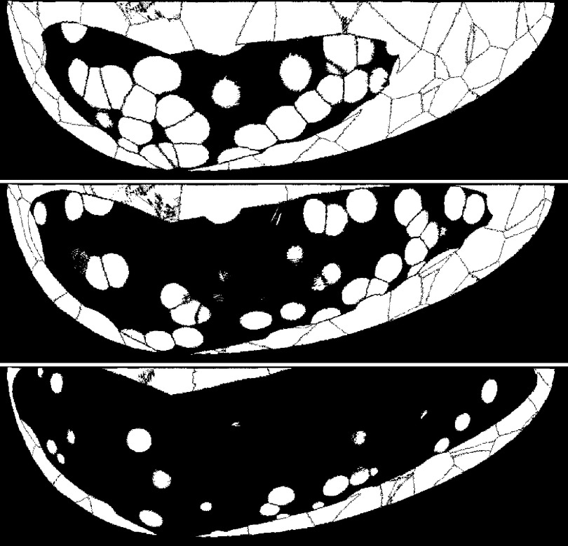
The backgrounds were differentiated by density. Breasts having low, medium, and high densities were defined with mean volumetric glandular percents (VGPs) of 25%, 50%, and 75%, respectively. According to Yaffe et al.,28 average breast glandularity for women of age 40 and higher is well below 50%, although measurements of nearly 75% for individual cases are possible. Different VGPs for the Bakic phantom were obtained by varying the size of the fibroglandular compartment. Figure 1 displays an example phantom slice for each mean VGP. Three background realizations were generated for each density. The exact VGP values for the phantoms were reported in Ref. 8, but each was within 3% of its respective mean.
FIG. 1.
Comparison of mean breast densities used in the study. From top to bottom are example slices from a low-density phantom (25% VGP), a medium-density phantom (50% VGP), and a high-density phantom (75% VGP). Within the breast regions, adipose tissue is white and glandular tissue is black.
Each background was used to create 16 test cases, with 8 single-mass (or abnormal) and 8 no-mass (or normal) cases, for a total of 9 × 16 = 144 cases. The masses were homogeneous spheres with an 8.0-mm diameter, randomly positioned within the fibroglandular compartment of the phantom. In creating the tumor phantoms, the partial volume effects were controlled by subsampling each voxel on a 10 × 10 × 10 grid. The attenuation coefficients for the masses modeled infiltrating ductal carcinoma as a function of energy, and were based on empirical measurements.29 The average contrast of the masses relative to background was only a few percent.
3.D. Data generation
The simulated DBT system modeled a rotating source-detector geometry with a step-and-shoot protocol. The cone-beam projector used Siddon ray-tracing30 to model x-ray transmission through the breast as described in Ref. 31. The subsequent propagation of signals and noise through a CsI-based amorphous silicon flat-panel detector was based on a serial cascade model that described (i) x-ray interactions with the scintillator, (ii) the generation, transport, and integration of optical quanta, and (iii) the addition of electronic noise.32 The focal-spot size was 100 μm. Scintillator blur was simulated with an empirically measured modulation transfer function for a CsI thickness of 100 μm, although the dependence of scintillator blur on angle of incidence was not included. Quantum noise was modeled by a Poisson distribution, while additive electronic noise followed a Gaussian process with a standard deviation of 2200 electrons. Scatter was not modeled in this simulation.
All imaging involved a filtered molybdenum spectra at 30 kVp (x-ray energies between 10 and 30 keV) as estimated using the methods described by Boone et al.33 The detector pixel size was 100 μm. We tested 12 acquisition protocols that used a fixed angular span of α = 60° and the number of projections P ∈ {3, 7, 11, 15, 19, 21, 25, 31, 35, 41, 45, 51}. The Poisson noise in each projection set was consistent with a mean glandular dose of 1.5 mGy equally distributed among the projections.
3.E. Image reconstruction
The raw projections were first normalized by the flood value and then converted to attenuation-coefficient integrals by taking the negative natural log. These processed projections were reconstructed by means of the Feldkamp filtered backprojection algorithm with a ramp filter.34 The 3D reconstruction dimensions were 760 × 240 × 195, with in-plane voxel dimensions of 0.27 × 0.27 mm. As the main objective of this work was to compare the model observers against human-observer data, no attempt was made to optimize the postprocessing. A fifth-order, 3D Butterworth filter with cutoff frequency fc = 0.25 pixel−1 was applied to the reconstructed volumes.
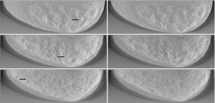
Test images for the observer study were produced by extracting slices that contained the center coordinates of the inserted masses. The neighboring four slices (two above and two below) were also extracted. These five slices were slabbed using boxcar smoothing to form the final test image with a 1-mm slice thickness, a process which is also used in clinic practice. The analogous slices for the corresponding lesion-free phantoms were also extracted. Each volume yielded one image, for a total of 72 normal/abnormal image pairs. These images were converted to 8-bit grayscale for presentation to the observers. No thresholding was applied. The sample images shown in Fig. 2 illustrate how mass detectability could vary with increasing breast density. Figure 3 compares the reconstructed images obtained from a given phantom for different values of P.
FIG. 2.
Example study images showing the impact of phantom VGP. From top to bottom, the left-hand column shows abnormal cases with 25%, 50%, and 75% VGP, respectively. The lesion in each image is indicated by the arrow. The corresponding normal images are shown at right. All images were generated from acquisitions with P = 25.
FIG. 3.
Example study images showing the effects of P. Shown is a same-slice comparison from FBP reconstructions generated from (a) P = 3, (b) 7, (c) 25, and (d) 51. This was a lesion-present case with 50% VGP. The lesion location is indicated by the arrow in the bottom left-hand image (P = 25).
3.F. LROC study
The human observer study evaluated the seven acquisition protocols corresponding to P ∈ {3, 7, 11, 15, 25, 35, 45}. LROC data were collected from three nonclinician observers. These observers had different levels of experience in reading simulated images, but all were knowledgeable about the goals of the study. There were 144 images per protocol (72 pairs of abnormal/normal images), divided into two sets of 54 study images (27 pairs) and 18 training images (9 pairs). Each observer thus read 14 image sets. The order in which these sets were read varied with observer, and the reading order of the images in a given set was randomized for each observer. The images were displayed on a computer monitor. Observers were not allowed to adjust the display but were permitted to vary both the room lighting and viewing distance. Ratings in the human study were collected on a four-point ordinal scale. Correct localizations were assessed with a 4-mm (14.8-pixel) radius of correct localization (RCL), equal to the radius of the spherical tumors.
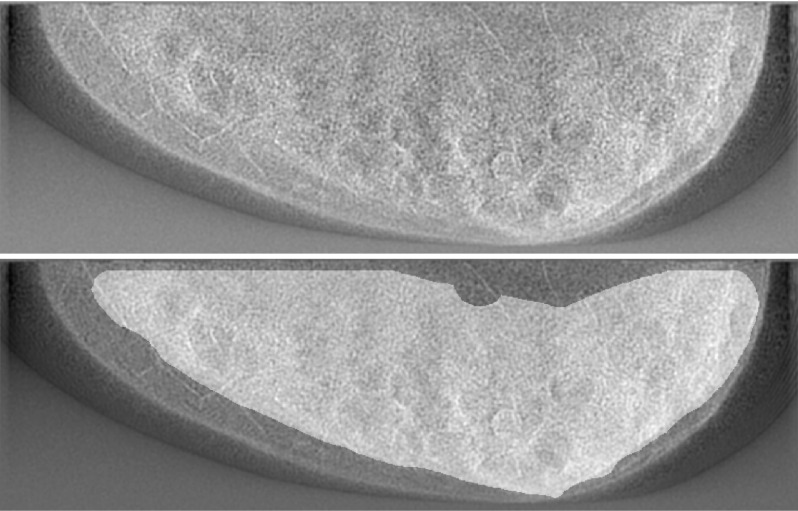
The various model observers read the same images as the human observers but were also applied for additional protocols defined by P ∈ {19,21,31,41,51}. Observer training for a given protocol consisted of estimating the mean reconstructed lesion profile and the mean background b. In this work, for a given protocol was estimated from the 36 training images, whereas b was approximated from the noise-free normal reconstructions associated with the training images. The search region Ω for a given f consisted of the pixels within the fibroglandular compartment (see Fig. 4). As indicated by Fig. 1, the average 2D search area increased with breast density. The model-observer rating data were maintained as floating-point values, as opposed to being converted to an ordinal scale. Correct localizations were assessed with the same RCL as in the human-observer study.
FIG. 4.
Example of search region used by model observers. Top: a test image; bottom: same image with fibroglandular search region highlighted.
For all observers, performance was quantified in terms of AL. The estimate of AL for a given observer and protocol was obtained with a Wilcoxon-based nonparametric ranking method.35 Each human observers data from the two image subsets were pooled prior to analysis. Standard errors for the AL estimates were calculated using the formula given in Ref. 36. The overall human performance for a given strategy was calculated as the average over the individual observers. A three-way analysis of variance (ANOVA) with reconstruction strategy, observer and phantom density as fixed factors was used to test the statistical significance of the results.
4. RESULTS
4.A. Human observers
The individual and average performances from the human observers (AL and , respectively) are summarized in Table I. The uncertainties in AL (not listed) were between 0.07 and 0.08. Nominally, the lowest and highest average performances were obtained with P = 3 and 25, respectively. An increase from 3 to 7 projections brought the greatest improvement in , and performances between 7 and 35 projections appeared relatively stable. The results also suggest that average observer performance had started to decline at the highest P, but addition data are needed to confirm this.
TABLE I.
Summary of overall and VGP-specific human-observer LROC performances in terms of AL and . The uncertainties in AL for the individual observers were between 0.07 and 0.08.
| P | ||||||||
|---|---|---|---|---|---|---|---|---|
| Observer | VGP | 3 | 7 | 11 | 15 | 25 | 35 | 45 |
| Human #1 | 0.25 | 0.78 | 0.86 | 0.94 | 1.0 | 0.98 | 1.0 | 1.0 |
| 0.50 | 0.50 | 0.69 | 0.63 | 0.58 | 0.71 | 0.54 | 0.39 | |
| 0.75 | 0.0 | 0.15 | 0.06 | 0.14 | 0.18 | 0.03 | 0.10 | |
| Overall | 0.42 | 0.57 | 0.54 | 0.57 | 0.63 | 0.52 | 0.50 | |
| Human #2 | 0.25 | 0.83 | 0.83 | 0.92 | 0.97 | 1.0 | 0.92 | 0.94 |
| 0.50 | 0.47 | 0.61 | 0.55 | 0.56 | 0.54 | 0.60 | 0.44 | |
| 0.75 | 0.0 | 0.19 | 0.0 | 0.05 | 0.17 | 0.08 | 0.0 | |
| Overall | 0.43 | 0.54 | 0.49 | 0.53 | 0.57 | 0.54 | 0.46 | |
| Human #3 | 0.25 | 0.89 | 0.83 | 0.94 | 0.89 | 0.99 | 0.94 | 1.0 |
| 0.50 | 0.44 | 0.64 | 0.51 | 0.61 | 0.66 | 0.49 | 0.53 | |
| 0.75 | 0.0 | 0.11 | 0.14 | 0.11 | 0.03 | 0.08 | 0.03 | |
| Overall | 0.44 | 0.53 | 0.53 | 0.54 | 0.56 | 0.51 | 0.52 | |
| Average | 0.43 ± 0.01 | 0.55 ± 0.02 | 0.52 ± 0.03 | 0.54 ± 0.02 | 0.58 ± 0.04 | 0.52 ± 0.02 | 0.49 ± 0.03 | |
Table I also presents a subanalysis of observer performance as a function of phantom VGP. As suggested by Fig. 2, VGP had a dramatic affect on performance, in part because the higher-density cases also presented larger search areas. Lesion detectability with the 75% cases was poor regardless of the choice of P. On the other hand, performance with the 25% cases maintained a relatively stable high level with P ≥ 11. For the mid-density cases (50% VGP), the highest performances were associated with intermediate values of P. The significance of this interaction between protocol and breast density was borne out by the three-way ANOVA. The analysis outcomes are presented in Table II. Along with the protocol–density interaction (p = 0.023), protocol (p = 4.3 × 10⁻⁴) and density (p = 2.2 × 10⁻¹⁶) as main effects were also statistically significant at the α = 0.05 level. None of the observer-related effects were significant.
TABLE II.
Results from the three-way ANOVA conducted with the human-observer scores. The analysis tested acquisition strategy, observer and phantom density as factors. The protocol and density effects, as well as the interaction between them, were significant at the α = 0.05 level. The corresponding p-values are indicated in boldface.
| Factor | df | ss | F | Pr(>F) |
|---|---|---|---|---|
| Protocol | 6 | 0.012 | 6.32 | 4.3×10⁻⁴ |
| Observer | 2 | 0.0086 | 1.34 | 0.28 |
| Density | 2 | 7.58 | 1179.61 | 2.2×10⁻¹⁶ |
| Protocol:observer | 12 | 0.016 | 0.42 | 0.94 |
| Protocol:density | 12 | 0.10 | 2.58 | 0.023 |
| Observer:density | 4 | 0.0008 | 0.06 | 0.99 |
| Residuals | 24 | 0.077 |
4.B. Model observers
4.B.1. Morphological features
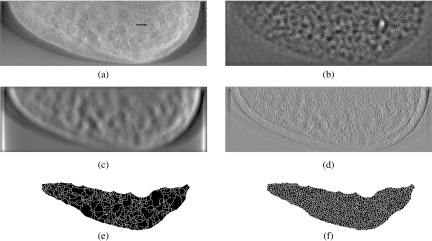
A lesion-present, mid-density test image is shown in Fig. 5(a), with the lesion indicated by the arrow in the right-central region. The CNPW, MF, and GMF correlation maps extracted from the image are shown in Figs. 5(b)–5(d), respectively. The calculations for all three features make use of the lesion profile but emphasize different ranges of spatial frequencies. Nonetheless, strong focal points corresponding with the lesion position are seen in each map. The watershed segmentations of the MF and GMF maps are seen in Figs. 5(e) and 5(f). The dark regions are the watershed supports and the white lines indicate the watershed boundaries. The focal points associated with the watersheds are the input to the candidate analysis for a VS observer.
FIG. 5.
Correlation-map calculations for the VS observers. (a) A lesion-present, mid-density test image. The lesion is indicated by the arrow. (b) CNPW correlation map; (c) MF correlation map; (d) GMF correlation map; (e) Watershed segmentation of the MF map; (f) Watershed segmentation of the GMF map. The dark regions in the segmentation images represent the watershed supports and the white lines are the watershed boundaries.
4.B.2. Study results
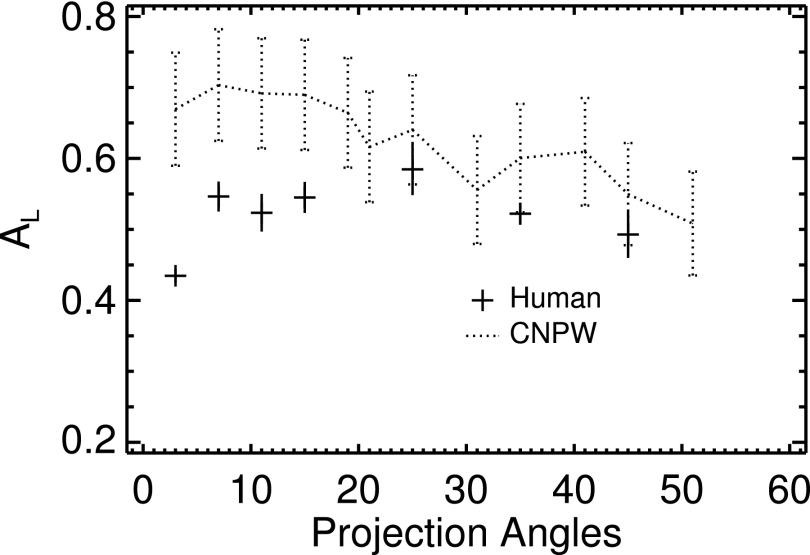
As described in Sec. 3, five base observer models were tested: the scanning CNPW observer and four VS observers (the MF–CNPW, GMF–CNPW, MF–GMF, and GMF–GMF versions). Figure 6 compares the CNPW and average human-observer results. The scanning observer carried out a BKE task that amounted to lesion detection in reconstructed quantum noise. As such, this observer was largely unaffected by the diminished lesion conspicuity that is evident in the images with low P (see Fig. 3). Instead, the trend in CNPW-observer performance reflects the increased levels of quantum noise in the images as P increased.
FIG. 6.
Comparison of performances from the scanning-CNPW and human observers.
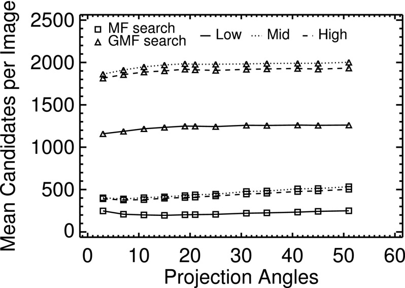
With the VS observers, both the search and analysis processes can influence performance. The MF and GMF statistics were used (separately) to control the search. One expects that the latter statistic would generate a noisier correlation map. Figure 7 shows how the average number of candidate locations varied with P and breast density as determined from unthresholded segmentation of the MF and GMF correlation maps, thus providing an empirical index of noise texture. As shown in this figure, the GMF statistic produced approximately four times as many candidate locations for a given P and phantom VGP as did the MF statistic. Regardless of which statistic was used, however, the number of candidates with the low-density phantoms was approximately half what were obtained with the mid- and high-density phantoms, in part because of the increased search area in the latter. As a function of P, the number of candidates was consistently highest with the mid-density phantoms, suggesting that the texture in the images from the high-density phantoms was of somewhat greater uniformity. Overall, the mean number of locations was not greatly affected by P.
FIG. 7.
Mean number of VS candidates per test image as a function of acquisition strategy (P), search feature and average phantom VGP. Data from the low-, mid-, and high-VGP phantoms are distinguished by the line style. With both search types, the low-density phantoms consistently yielded the fewest candidates. The mid-density phantoms consistently produced the most candidates, slightly more than with the high-density phantoms.
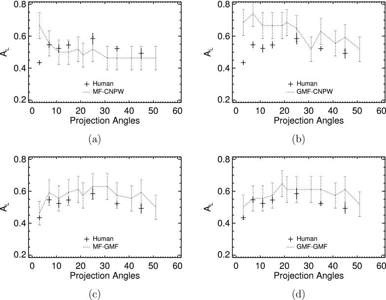
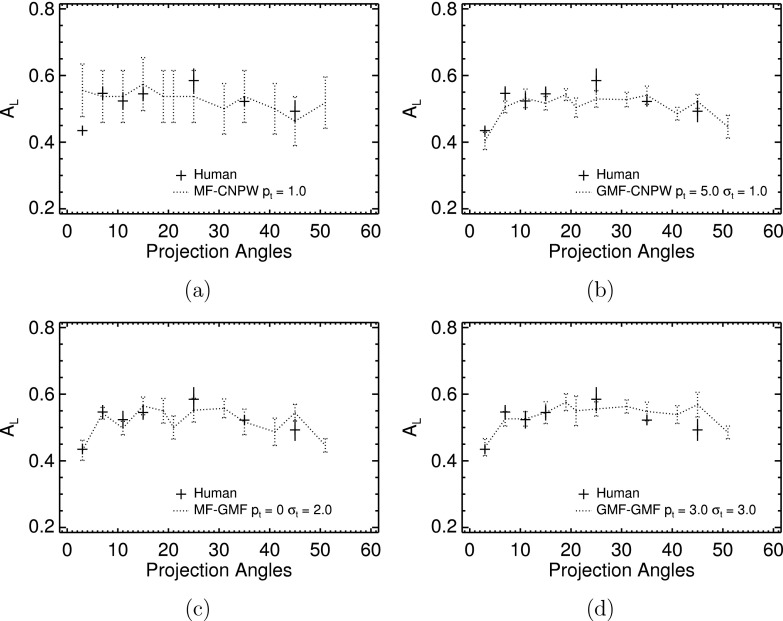
Results for the VS observers operated without the search threshold or noise processes defined by pt and σt are plotted against average human-observer performances in Fig. 8. These plots indicate that the differences between the MF and GMF search outputs had less effect on model performance than did the form of candidate analysis. Both CNPW-based models [Figs. 8(a) and 8(b)] displayed trends in AL that emulated the scanning observer to some degree. With the GMF–CNPW observer, the agreement was quite high due to the prolific search that for low P usually included the actual lesion location. In comparison, performances with the MF–CNPW version decreased rapidly with increasing P, with the observer tending to underestimate human-observer scores for P > 10.
FIG. 8.
Comparison of observer performances from the VS and human observers. (a) The MF–CNPW observer; (b) the GMF–CNPW observer; (c) the MF–GMF observer; and (d) the GMF–GMF observer. The search thresholding and noise processes were not implemented with the VS models for these plots.
With GMF analysis [Figs. 8(c) and 8(d)], search type did not substantially affect observer performance. Given this, we see that the problem with the MF–CNPW observer is not that the search excludes relatively high numbers of actual lesion locations. Instead, the difference with the GMF–CNPW observer lies in the higher number of focal points per unit area that the GMF search returns. The net effect is heightened sampling of the CNPW statistic of Eq. (15) in the vicinity of a lesion location, which increases the probability with abnormal images that the maximum of zj will yield a true-positive localization. This advantage of oversampling is largely negated with the GMF analysis, which generates correlation maps with less-diffuse blobs compared to the CNPW maps (cf. Fig. 5). In such cases, the relatively conservative MF search is adequate for sampling the true lesion locations. The Pearson correlation coefficient between the human and MF–GMF results in Fig. 8(c) was 0.79. The coefficient was 0.62 for the GMF–GMF observer. These results with the GMF analysis indicate the useful information to be gained from some VS models even without thresholding the large numbers of candidate locations (see Fig. 7).
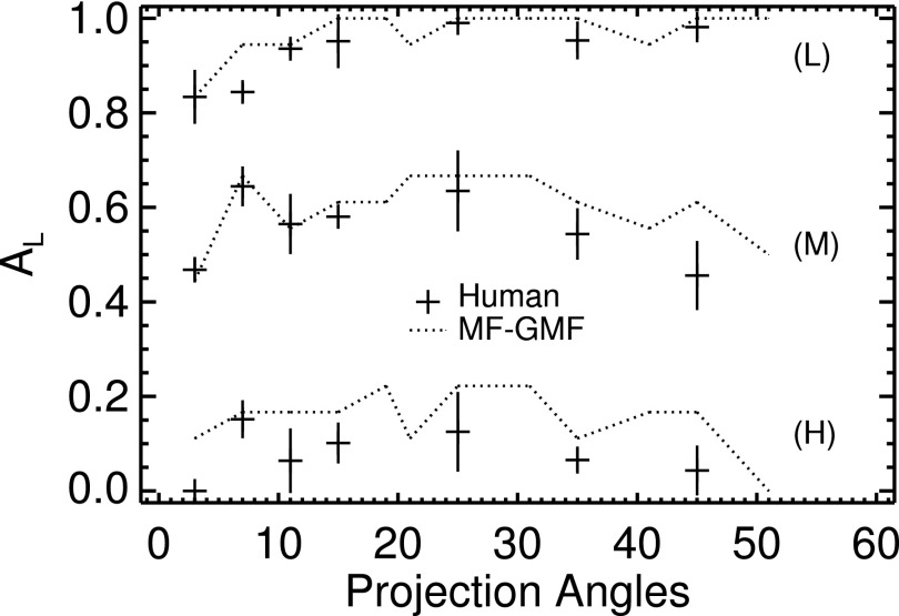
A subanalysis of observer performance based on phantom density was carried out with the two VS observers that relied on GMF analysis. As indicated in Fig. 9 for the MF–GMF model, these observers demonstrated responses to variations in VGP and search area that were largely similar on average to those of the human observers.
FIG. 9.
Comparison of VS and human observer performances as a function of phantom density. The densities are denoted in the plot as low (L), medium (M) and high (H). The average 2D search area in the images increased with density.
To examine the relative effects of quantum and anatomical noise on observer performance in this study, we may treat the GMF–CNPW observer as being quasi-ideal owing to its BKE assumption. According to Fig. 8, the GMF–GMF observer performances largely coincided for P ≳ 21, indicating that quantum noise was the principal factor in that range while anatomical noise effects dominated for smaller P values. Further studies are necessary to assess the separate influences of acquisition arc length and reconstruction method on anatomical noise.
Experiments with incorporating search inefficiencies in the VS models were focused on fitting the human-observer data by varying the pt and σt parameters. As noted in Sec. 3.B.3, 24 pairs of these parameters were tested. For a given parameter choice, observer performance was computed as a function of P. When σt was nonzero, observer performance was computed for a given P as the average performance from ten study realizations. The plots in Fig. 10 indicate the magnitudes of pt and σt that were required to fit the human data with each VS observer. With the MF–CNPW model [Fig. 10(a)], nonzero σt or pt > 1 led to underestimation of the human performances for most P. The other three models could approximate the human data with various parameter combinations. Higher levels of thresholding were required to penalize the high sampling obtained with the GMF search [Figs. 10(b) and 10(d)], regardless of which candidate analysis was used. The MF–GMF model [Fig. 10(c)] used relatively lower parameter values.
FIG. 10.
Comparison of VS and human observer performances when the models included the search thresholding and noise processes controlled by pt and σt, respectively. (a) The MF–CNPW observer; (b) the GMF–CNPW observer; (c) the MF–GMF observer; and (d) the GMF–GMF observer. The model-observer error bars for the nonzero σt examples indicate the standard deviation in AL from ten study realizations.
5. DISCUSSION
Model observers are primarily intended for system evaluation and optimization, but obtaining meaningful results with them requires realistic images and task definitions. Extensive prior studies of DBT imaging have applied observers under various location-known settings, but to what degree such relatively simple tasks can reliably predict outcomes for more clinically realistic tasks has not been extensively studied. To our knowledge, the current work offers the first validation of a search-capable model observer that accounts for both quantum and anatomical noise in DBT reconstructions. The training requirements for the VS observer are well-suited for high-resolution x-ray imaging: all four versions of the observer in this study used 36 training images per test strategy for estimating the lesion profile, and the MF–GMF and GMF–GMF versions did not require information about the mean image backgrounds.
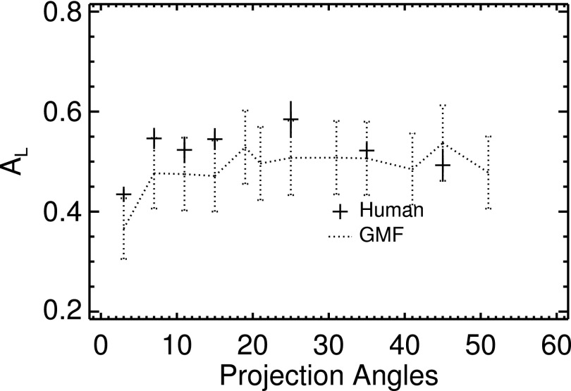
The findings with the GMF–GMF observer in this study might suggest that a basic scanning GMF observer (without background subtraction) could serve in place of the two-stage VS framework to predict human performance, but Fig. 11 indicates otherwise. Overall, the VS paradigm offers considerable advantages for analyzing detection-localization tasks, with several studies having shown improved stability compared to scanning models in situations where organ-boundary artifacts interfered with detection.37 There were strong limited-angle artifacts at the borders of the fibroglandular compartment in some of the test images, and while some effort was made to control their impact on the feature extraction, this was not completely successful.
FIG. 11.
Human and scanning-GMF performances. Compare with the GMF–GMF observer results in Fig. 8(d).
The VS observers used morphological target features to compute the correlation maps for the candidate search. These maps quantify image stimuli like contrast and edge orientation subject to prior knowledge of the target. Put another way, each map indicates how the saliency of a given feature (or task-independent image visibility38) interacts with an observer’s knowledge of the target. Candidate locations are indicated by local correlation maxima, but many are attributable to noise texture alone. Thus, if the selected features adequately summarize how humans recognize a target, then the outcome of the candidate search may mimic the effects of noise texture on human-observer search results. In poststudy discussions, our human observers have related that edge detection provided the only reliable clue about lesion presence in the mid- and high-density phantoms. This observation was verified in a separate analysis of eye-tracking data that examined the correlations between observer dwell time at fixation points with the various search statistics computed in this paper.39
The relative importance of specific features such as the GMF naturally depends on what is being imaged and how the images are acquired. The FBP images in our study featured low-contrast, symmetric targets with high levels of background noise, and it is reasonable to expect that the GMF-based VS observers would also serve for detecting nonsymmetric or different-sized targets in the same backgrounds. On the other hand, iterative DBT reconstructions can present relatively complex noise texture, with anatomical distractors more apparent due to reduced statistical noise. Addressing this with the VS observer will likely require integrating information from multiple features as part of both the search and analysis stages.
We reiterate that this study comprises only an initial validation of VS observers for DBT. Further DBT studies are investigating the image-quality effects of scan arc and dose level.40 A fully general validation of an observer model involves training on one set of cases and testing on a different set, thus requiring an expanded population of breast and lesion phantoms (including microcalcification models). The present study reduced what is typically a volumetric search task to a 2D problem, and in doing so may have obscured important differences between the acquisition configurations. VS observers for static-frame reading of multislice images may be constructed by following the methods in Ref. 15. Several researchers (e.g., Ref. 41) have tested model observers with scrolling capabilities and we shall investigate the same for the VS observers.
The ultimate goal of this research is to develop reliable human-observer models that are not predicated on extensive prior knowledge. The VS models are nonideal in the sense that prior knowledge about the noise properties has not been utilized. In comparison, the CH observer uses ensemble statistics to account for the effects of noise (Sec. 2.F). By responding more on an image-by-image basis, the VS observer provides a unique means for comparing tasks based not only on what the observer must do with the image but also on the observer’s prior knowledge. One objective will be to examine how system optimizations can differ using these human-observer models as opposed to ideal observers.42 Note also that human observers have long been modeled as ideal observers degraded by internal noise. With CH observers, the internal noise is generally added by modifying the ensemble covariance matrices. As indicated by the use of the search threshold and noise processes in this study, the VS framework provides a richer environment for studying human-observer inefficiencies. Among the questions to be considered are which imaging parameters are most sensitive to these inefficiencies and whether variations in the inefficiency parameters can be used to describe individual humans.
6. CONCLUSIONS
Initial validation of several VS observer models for DBT imaging has been presented, with several versions of the model demonstrating good agreement with limited human-observer data. The VS observers do not require covariance information. The observer training requirements are suitable for high-resolution imaging applications, indicating that the VS framework has the potential to overcome important limitations of current search-capable model observers.
ACKNOWLEDGMENTS
Predrag Bakic of the University of Pennsylvania supplied the anthropomorphic breast phantoms used for this study. This work was supported by the National Cancer Institute under Grant No. K25-CA140858 and the National Institute for Biomedical Imaging and Bioengineering under Grant No. R01-EB12070. The contents are solely the responsibility of the authors and do not necessarily represent the views of these institutes.
REFERENCES
- 1.Anastasio M. A., Chou C.-Y., Zysk A. M., and Brankov J. G., “Analysis of ideal observer signal detectability in phase-contrast imaging employing linear shift-invariant optical systems,” J. Opt. Soc. Am. A 27, 2648–2659 (2010). 10.1364/JOSAA.27.002648 [DOI] [PMC free article] [PubMed] [Google Scholar]
- 2.Zysk A. M., Brankov J. G., Wernick M. N., and Anastasio M. A., “Adaptation of a clustered lumpy background model for task-based image quality assessment in x-ray phase-contrast mammography,” Med. Phys. 39, 906–911 (2012). 10.1118/1.3676183 [DOI] [PMC free article] [PubMed] [Google Scholar]
- 3.Packard N. J., Abbey C. K., Yang K., and Boone J. M., “Effect of slice thickness on detectability in breast CT using a prewhitened matched filter and simulated mass lesions,” Med. Phys. 39, 1818–1830 (2012). 10.1118/1.3692176 [DOI] [PMC free article] [PubMed] [Google Scholar]
- 4.Reiser I. S. and Nishikawa R. M., “Task-based assessment of breast tomosynthesis: Effect of acquisition parameters and quantum noise,” Med. Phys. 37, 1591–1600 (2010). 10.1118/1.3357288 [DOI] [PMC free article] [PubMed] [Google Scholar]
- 5.Das M. and Gifford H. C., “Comparison of model-observer and human-observer performance for breast tomosynthesis: Effect of reconstruction and acquisition parameters,” Proc. SPIE 7961, 796118 (2011). 10.1117/12.878826 [DOI] [Google Scholar]
- 6.Zhang Y., Pham B. T., and Eckstein M. P., “Evaluation of internal noise methods for Hotelling observer models,” Med. Phys. 34, 3312–3322 (2007). 10.1118/1.2756603 [DOI] [PubMed] [Google Scholar]
- 7.Gazelle G. S., Seltzer S. E., and Judy P. F., “Assessment and validation of imaging methods and technologies,” Acad. Radiol. 10, 894–896 (2003). 10.1016/S1076-6332(03)00062-X [DOI] [PubMed] [Google Scholar]
- 8.Gifford H. C., Didier C. S., Das M., and Glick S. J., “Optimizing breast-tomosynthesis acquisition parameters with scanning model observers,” Proc. SPIE 6917, 69170S (2008). 10.1117/12.771018 [DOI] [Google Scholar]
- 9.Popescu L. M. and Myers K. J., “CT image assessment by low contrast signal detectability evaluation with unknown signal location,” Med. Phys. 40, 111908(10 pp.) (2013). 10.1118/1.4824055 [DOI] [PubMed] [Google Scholar]
- 10.Handbook of Medical Imaging: Physics and Psychophysics, edited by Beutel J., Kundel H. L., and Van Metter R. L. (SPIE, Bellingham, WA, 2000). [Google Scholar]
- 11.Eckstein M. P. and Abbey C. K., “Model observers for signal-known-statistically tasks (SKS),” Proc. SPIE 4324, 91–102 (2001). 10.1117/12.431177 [DOI] [Google Scholar]
- 12.Gifford H. C., Wells R. G., and King M. A., “A comparison of human observer LROC and numerical observer ROC for tumor detection in SPECT images,” IEEE Trans. Nucl. Sci. 46, 1032–1037 (1999). 10.1109/23.790820 [DOI] [Google Scholar]
- 13.Kundel H. L., Nodine C. F., Conant E. F., and Weinstein S. P., “Holistic component of image perception in mammogram interpretation: Gaze-tracking study,” Radiology 242, 396–402 (2007). 10.1148/radiol.2422051997 [DOI] [PubMed] [Google Scholar]
- 14.Eckstein M. P., “Visual search: A retrospective,” J. Vision 11, 1–36 (2011). 10.1167/11.5.14 [DOI] [PubMed] [Google Scholar]
- 15.Gifford H. C., “A visual-search model observer for multislice-multiview SPECT images,” Med. Phys. 40, 092505 (12 pp.) (2013). 10.1118/1.4818824 [DOI] [PMC free article] [PubMed] [Google Scholar]
- 16.Chawla A. S., Lo J. Y., Baker J. A., and Samei E., “Optimized image acquisition for breast tomosynthesis in projection and reconstruction space,” Med. Phys. 36, 4859–4869 (2009). 10.1118/1.3231814 [DOI] [PMC free article] [PubMed] [Google Scholar]
- 17.Park S., Zhang G. Z., and Zeng R., “Comparing observer models and feature selection methods for a task-based statistical assessment of digital breast tomsynthesis in reconstruction space,” Proc. SPIE 9037, 90370M (2014). 10.1117/12.2043598 [DOI] [Google Scholar]
- 18.Samei E., Thompson J., Richard S., and Bowsher J., “A case for wide-angle breast tomosynthesis,” Acad. Radiol. 22, 860–869 (2015). 10.1016/j.acra.2015.02.015 [DOI] [PubMed] [Google Scholar]
- 19.Lau B. A., Das M., and Gifford H. C., “Towards visual-search model observers for mass detection in breast tomosynthesis,” Proc. SPIE 8668, 86680X (2013). 10.1117/12.2008503 [DOI] [PMC free article] [PubMed] [Google Scholar]
- 20.Barrett H. H., Furenlid L. R., Freed M., Hesterman J. Y., Kupinski M. A., Clarkson E. W., and Whitaker M. K., “Adaptive SPECT,” IEEE Trans. Med. Imaging 27, 775–788 (2008). 10.1109/TMI.2007.913241 [DOI] [PMC free article] [PubMed] [Google Scholar]
- 21.Khurd P. and Gindi G. R., “Decision strategies that maximize the area under the LROC curve,” IEEE Trans. Med. Imaging 24, 1626–1636 (2005). 10.1109/TMI.2005.859210 [DOI] [PubMed] [Google Scholar]
- 22.Kupinski M. A., Hoppin J. W., Clarkson E. W., and Barrett H. H., “Ideal-observer computation in medical imaging with use of Markov-chain Monte Carlo techniques,” J. Opt. Soc. Am. A 20, 430–438 (2003). 10.1364/JOSAA.20.000430 [DOI] [PMC free article] [PubMed] [Google Scholar]
- 23.Gifford H. C., Kinahan P. E., Lartizien C., and King M. A., “Evaluation of multiclass model observers in PET LROC studies,” IEEE Trans. Nucl. Sci. 54, 116–123 (2007). 10.1109/TNS.2006.889163 [DOI] [PMC free article] [PubMed] [Google Scholar]
- 24.Roerdink J. B. T. M. and Meijster A., “The watershed transform: Definitions, algorithms and parallelization strategies,” Fundam. Inf. 41, 187–228 (2000). 10.3233/FI-2000-411207 [DOI] [Google Scholar]
- 25.Shapley R. M. and Tolhurst D. J., “Edge detectors in human vision,” J. Physiol. 229, 165–183 (1973). 10.1113/jphysiol.1973.sp010133 [DOI] [PMC free article] [PubMed] [Google Scholar]
- 26.Jain A. K., Fundamentals of Digital Image Processing (Prentice Hall, Upper Saddle River, NJ, 1988). [Google Scholar]
- 27.Bakic P. R., Albert M., Brzakovic D., and Maidment A. D. A., “Mammogram synthesis using a 3D simulation. I. Breast tissue model and image acquisition simulation,” Med. Phys. 29, 2131–2139 (2002). 10.1118/1.1501143 [DOI] [PubMed] [Google Scholar]
- 28.Yaffe M. J., Boone J. M., Packard N. J., Alonzo-Proulx O., Huang S. Y., Peressotti C. L., Al-Mayah A., and Brock K., “The myth of the 50-50 breast,” Med. Phys. 36, 5437–5443 (2009). 10.1118/1.3250863 [DOI] [PMC free article] [PubMed] [Google Scholar]
- 29.Johns P. C. and Yaffe M. J., “X-ray characterisation of normal and neoplastic breast tissues,” Phys. Med. Biol. 32, 675–695 (1987). 10.1088/0031-9155/32/6/002 [DOI] [PubMed] [Google Scholar]
- 30.Siddon R. L., “Fast calculation of the exact radiological path for a three-dimensional CT array,” Med. Phys. 12, 252–255 (1985). 10.1118/1.595715 [DOI] [PubMed] [Google Scholar]
- 31.Gong X., Glick S. J., Liu B., Vedula A. A., and Thacker S., “A computer simulation study comparing lesion detection accuracy with digital mammography, breast tomosynthesis, and cone-beam CT breast imaging,” Med. Phys. 33, 1041–1052 (2006). 10.1118/1.2174127 [DOI] [PubMed] [Google Scholar]
- 32.Vedula A. A., Glick S. J., and Gong X., “Computer simulation of CT mammography using a flat-panel imager,” Proc. SPIE 5030, 349–360 (2003). 10.1117/12.480015 [DOI] [Google Scholar]
- 33.Boone J. M., Fewell T. R., and Jennings R. J., “Molybdenum, rhodium, and tungsten anode spectral models using interpolating polynomials with application to mammography,” Med. Phys. 24, 1863–1874 (1997). 10.1118/1.598100 [DOI] [PubMed] [Google Scholar]
- 34.Feldkamp L. A., Davis L. C., and Kress J. W., “Practical cone-beam algorithm,” J. Opt. Soc. Am. A 1, 612–619 (1984). 10.1364/JOSAA.1.000612 [DOI] [Google Scholar]
- 35.Hanley J. A. and McNeil B. J., “The meaning and use of the area under a receiver operating characteristic (ROC) curve,” Radiology 143, 29–36 (1982). 10.1148/radiology.143.1.7063747 [DOI] [PubMed] [Google Scholar]
- 36.Tang L. L. and Balakrishnan N., “A random-sum Wilcoxon statistic and its application to analysis of ROC and LROC data,” J. Stat. Plann. Inference 141, 335–344 (2011). 10.1016/j.jspi.2010.06.011 [DOI] [PMC free article] [PubMed] [Google Scholar]
- 37.Gifford H. C., “Efficient visual-search model observers for PET,” Br. J. Radiol. 87, 20140017 (2014). 10.1259/bjr.20140017 [DOI] [PMC free article] [PubMed] [Google Scholar]
- 38.Itti L. and Koch C., “Computational modelling of visual attention,” Nat. Rev. Neurosci. 2, 194–203 (2001). 10.1038/35058500 [DOI] [PubMed] [Google Scholar]
- 39.Jiang Z., Liang Z., Das M., and Gifford H. C., “Towards using eye-tracking data to develop visual-search observers for x-ray breast imaging,” Proc. SPIE 9416, 94160V (2015). 10.1117/12.2082978 [DOI] [Google Scholar]
- 40.Das M., Liang Z., and Gifford H. C., “Clinically relevant task-based assessment for digital breast tomosynthesis using an adaptive visual-search model observer,” in Proceedings of the 2015 International Meeting on Fully Three-Dimensional Image Reconstruction in Radiology and Nuclear Medicine (Newport, RI, 2015), pp. 59–62. [Google Scholar]
- 41.Diaz I., Schmidt S., Verdun F. R., and Bochud F. O., “Eye-tracking of nodule detection in lung CT volumetric data,” Med. Phys. 42, 2925–2932 (2015). 10.1118/1.4919849 [DOI] [PubMed] [Google Scholar]
- 42.Sen A. and Gifford H. C., “Accounting for anatomical noise in search-capable model observers for planar nuclear imaging,” J. Med. Imaging 3, 015502 (2016). 10.1117/1.JMI.3.1.015502 [DOI] [PMC free article] [PubMed] [Google Scholar]


