Abstract
Purpose:
The authors have recently developed a preconditioned alternating projection algorithm (PAPA) with total variation (TV) regularizer for solving the penalized-likelihood optimization model for single-photon emission computed tomography (SPECT) reconstruction. This algorithm belongs to a novel class of fixed-point proximity methods. The goal of this work is to investigate how PAPA performs while dealing with realistic noisy SPECT data, to compare its performance with more conventional methods, and to address issues with TV artifacts by proposing a novel form of the algorithm invoking high-order TV regularization, denoted as HOTV-PAPA, which has been explored and studied extensively in the present work.
Methods:
Using Monte Carlo methods, the authors simulate noisy SPECT data from two water cylinders; one contains lumpy “warm” background and “hot” lesions of various sizes with Gaussian activity distribution, and the other is a reference cylinder without hot lesions. The authors study the performance of HOTV-PAPA and compare it with PAPA using first-order TV regularization (TV-PAPA), the Panin–Zeng–Gullberg one-step-late method with TV regularization (TV-OSL), and an expectation–maximization algorithm with Gaussian postfilter (GPF-EM). The authors select penalty-weights (hyperparameters) by qualitatively balancing the trade-off between resolution and image noise separately for TV-PAPA and TV-OSL. However, the authors arrived at the same penalty-weight value for both of them. The authors set the first penalty-weight in HOTV-PAPA equal to the optimal penalty-weight found for TV-PAPA. The second penalty-weight needed for HOTV-PAPA is tuned by balancing resolution and the severity of staircase artifacts. The authors adjust the Gaussian postfilter to approximately match the local point spread function of GPF-EM and HOTV-PAPA. The authors examine hot lesion detectability, study local spatial resolution, analyze background noise properties, estimate mean square errors (MSEs), and report the convergence speed and computation time.
Results:
HOTV-PAPA yields the best signal-to-noise ratio, followed by TV-PAPA and TV-OSL/GPF-EM. The local spatial resolution of HOTV-PAPA is somewhat worse than that of TV-PAPA and TV-OSL. Images reconstructed using HOTV-PAPA have the lowest local noise power spectrum (LNPS) amplitudes, followed by TV-PAPA, TV-OSL, and GPF-EM. The LNPS peak of GPF-EM is shifted toward higher spatial frequencies than those for the three other methods. The PAPA-type methods exhibit much lower ensemble noise, ensemble voxel variance, and image roughness. HOTV-PAPA performs best in these categories. Whereas images reconstructed using both TV-PAPA and TV-OSL are degraded by severe staircase artifacts; HOTV-PAPA substantially reduces such artifacts. It also converges faster than the other three methods and exhibits the lowest overall reconstruction error level, as measured by MSE.
Conclusions:
For high-noise simulated SPECT data, HOTV-PAPA outperforms TV-PAPA, GPF-EM, and TV-OSL in terms of hot lesion detectability, noise suppression, MSE, and computational efficiency. Unlike TV-PAPA and TV-OSL, HOTV-PAPA does not create sizable staircase artifacts. Moreover, HOTV-PAPA effectively suppresses noise, with only limited loss of local spatial resolution. Of the four methods, HOTV-PAPA shows the best lesion detectability, thanks to its superior noise suppression. HOTV-PAPA shows promise for clinically useful reconstructions of low-dose SPECT data.
Keywords: SPECT reconstruction, penalized maximum-likelihood optimization, high-order total-variation regularization, fixed-point proximity methods, noise suppression, staircase artifacts
1. INTRODUCTION
Single-photon emission computed tomography (SPECT) is a tomographic-imaging technique1 widely used in nuclear medicine for diagnostic imaging. In a SPECT camera, the detector records the number of collimated single gamma photons emitted by a radiotracer distributed inside a patient’s body. The collection of such emission data is sorted into a set of 2D projection images. Tomographic reconstruction of SPECT data can provide diagnostic information via estimates of the spatial and/or temporal distribution of radiotracers.
Because of the increased use of CT, nuclear medicine studies, and interventional medical procedures, the effective dose per individual in the United States increased more than sixfold over the past 30 yr.2 The nuclear medicine contributed 26% of per-capita dose increase. There are enormous benefits of radionuclide imaging. However, to truly realize them, the exams need to be optimized to achieve the best image quality with the lowest radiation dose.3 It can be accomplished via hardware improvement4–6 and/or new reconstruction methods implementation.7 In the present work, we focus on image quality improvement in the lower-dose SPECT studies by implementation of our new reconstruction method.
Many existing reconstruction methods for SPECT imaging are based on optimizing an objective function, deduced in part from a statistical model of projection data. For example, the maximum-likelihood (ML) criterion is based on minimizing the negative log-likelihood of observed emission data conditional on radiotracer activity distribution.8,9 Under the Bayesian framework, the maximum a posteriori (MAP) estimator seeks to minimize the sum of the negative log-likelihood of observed emission data conditional on radiotracer distribution and a regularizing penalty function, which penalizes solutions that have low probability.10,11 With various pursuits, such as improvement of computational efficiency of the algorithm, suppression of image noise, and preservation of image spatial resolution, different types of penalty functions have been proposed. The total variation (TV) penalty function, first proposed by Rudin et al.12 and introduced to the field of SPECT image reconstruction by Panin, Zeng, and Gullberg,13 is particularly interesting because it preserves the high frequency components of the reconstructed radiopharmaceutical distribution, including discontinuities and steep gradients. Efficient algorithms were proposed to solve the resultant regularization model, such as expectation–maximization (EM)-type methods,13–15 projected quasi-Newton methods,16–18 primal–dual approaches,19–21 and fixed-point proximity methods (TV-PAPA).22 However, images resulting from the application of the TV regularization in the presence of noise often have “blocky” appearance (i.e., appear as a collection of piecewise constant regions), so the finer details in the original image may not be recovered satisfactorily. In addition, reconstructed smooth transitions (weak gradients) of activity may contain piecewise constant regions called “staircase” artifacts. All these issues limit the clinical use of TV regularization. In order to suppress staircase artifacts, as well as to preserve the spatial resolution of the reconstructed image, we propose a high-order TV (HOTV) regularization model for SPECT reconstruction. Furthermore, we apply the preconditioned alternating projection algorithm (PAPA), originally developed for solving the TV model,22 to solving the HOTV model, thereby offering an efficient reconstruction method (HOTV-PAPA) for obtaining diagnostic quality images.
In the present work, we evaluate selected aspects of the reconstruction performance of HOTV-PAPA and compare them with those of TV-PAPA, the Panin–Zeng–Gullberg one-step-late method with the TV regularization (TV-OSL),13 and the widely used, conventional maximum-likelihood expectation maximization algorithm8 with Gaussian postfilter (GPF-EM). In order to best explore the effect of HOTV-PAPA on resolution, we simulate low-energy ultrahigh resolution (LEUR) fan-beam collimation, often used for brain imaging.
2. MATERIALS AND METHODS
2.A. Penalized maximum likelihood estimation for SPECT reconstruction
It is well established that the rate of disintegration of and subsequent gamma photon emission rate from an ensemble of radionuclei follows a temporal Poisson distribution. Since photon detections by different detector units during a SPECT scan are mutually independent events and can be described by a Bernoulli process23 (a discrete distribution having two possible outcomes), the projection images are a collection of independent Poisson random variables. The Poisson distribution approximates the photon-detection process only if one can neglect the detector dead time, and no corrections are applied to the raw data. Thus, in a SPECT system, the projection data g ∈ ℝm on m detector units, which is a random vector with independent entries and relates to the unobservable expected radiotracer activity distribution vector (called image) f ∈ ℝd in d voxels of the reconstruction volume, can be approximated by the Poisson model,1,24
| (1) |
In Eq. (1), Poisson(α) denotes a Poisson-distributed random vector with mean α, A is the m × d SPECT system matrix with its (i, j)th entry equal to the probability of detection of the photon emitted from voxel j of image f by the ith detector, and γ ∈ ℝm is the vector containing expected counts due to background activity (e.g., scattered photons coming from outside the field of view of the gamma camera or from room background).
Given a realization of the observed data g, the objective of SPECT reconstruction is to estimate an image f while suppressing Poisson noise and preserving spatial resolution. We formulate the reconstruction problem via the penalized ML criterion. Indeed, the penalized ML estimate is obtained by maximizing the sum of the log-likelihood function of f and the negative penalty term.10,11,25 Since the underlying likelihood function is assumed to be in a Poisson form described above, our proposed optimization model for SPECT reconstruction reads22
| (2) |
The data fidelity term , denoted by F in Secs. 2.B–2.H, is the Kullback-Leibler (KL) data divergence.26 The penalty (regularization) term λU is introduced to arrive at a realistic solution, i.e., to enforce desired smoothness of the estimate. It penalizes solutions with low probability. Here, λ is a positive regularization parameter, and U is the real-valued energy function. The details on formulation of U are presented in Sec. 2.B. Note that the constraint f ≥ 0 is required, because the expected radiotracer activity distribution vector f has all non-negative components.
2.B. The TV and high-order TV regularization terms
In this paper, we explore the TV and high-order TV regularization methods. The advantage of using the TV seminorm as a penalty function, over some other common regularization approaches that rely on various forms of the quadratic energy function, is that it does not penalize discontinuities, and thus allows preservation of sharp edges in the estimated activity distribution. However, besides sharp edges (the high frequency components), the radiotracer distribution f in patients also contains regions where it is a smooth function with respect to spatial coordinates. It is well known that the TV regularizer tends to reconstruct such regions as a collection of piecewise constant regions.27 This phenomenon, known as staircase artifacts, has severely limited clinical use of the TV regularization. To ameliorate the staircasing artifacts caused by TV, one can relax the first-order discontinuity by including higher-order discontinuity penalties. This can be achieved by taking higher-order derivatives into account. Successful applications of high-order derivative regularization methods can be found in Benning27 et al., Bredis28 et al., and Chan29 et al. In the present work, we limit ourselves to the approach that directly adds to the TV regularizer, a penalty term that depends on the second-order derivative of the image. In what follows, we briefly review the formulations of the TV and second-order TV regularizers.
Let f be a 3D image of size p × p × q. There are two possible definitions of the TV regularizers that have appeared in the literature. The first one, called anisotropic TV (ATV), is defined by the formula
while the second definition of total variation, called isotropic TV (ITV), is defined by
In numerical simulations, we observed that the ITV can better recover smooth surfaces (e.g., spheres or ellipsoids) in the estimated radiotracer activity distribution, while the ATV favors cuboid or rhombohedron surfaces in the image. Since the surfaces of most objects within clinical applications are sufficiently regular in the sense that they can be thought of as locally being the graphs of smooth functions, we only studied ITV in the present work.
Because images are represented as vectors in optimization model (2), it will be useful to vectorize the 3D image in the definition of ITV. Indeed, an image of size p × p × q can be treated as a vector in ℝp2q in such a way that the ijkth voxel of the image corresponds to the (i + (j − 1) p + (k − 1) p2)th component of the vector. In the current context, we set d = p2q.
For the sake of notational simplicity and algorithm development convenience, we next introduce a discrete gradient operator on the vectorized image and formulate the ITV regularizer as a composite function. Let Iα denote the α × α identity matrix, and Dα denote the α × α backward difference matrix with the Neumann boundary condition, which is defined by
In terms of the notion of Kronecker tensor product ⊗, we define the discrete gradient operator B1 by
As a result, recalling the vector representation of image f, we can rewrite the ITV regularizer as
Hence, by defining a convex function φ1 : ℝ3d → ℝ as , we can calculate the ITV regularizer as composition φ1∘B1.30
Next, following the notation used in Micchelli30 et al. and Setzer31 et al., we define the discrete partial second-order derivative operators as
We then stack the above matrices together and propose the following discrete second-order gradient operator:
| (3) |
Similar to ITV, if we define a convex function φ2 : ℝ9d → ℝ as , the composition φ2∘B2 computes the second-order derivative penalty term. With the above preparation, the second-order TV regularizer considered in this paper has the form
| (4) |
Note that, in either case when U is specified as TV or the second-order TV regularizer, the objective function in Eq. (2) is nondifferentiable. Therefore, traditional gradient-type and expectation maximization-type algorithms fail to solve the desired optimization problem. We emphasize that we have implemented an advanced approach based on the proximity operator, and our method does not require introduction of ad hoc parameters as has been done in the past in order to deal with nondifferentiability.13,17,18 This new approach has profound consequences for the algorithm’s performance.
2.C. Numerical algorithm
Nondifferentiable optimization problem (2) can be solved by the PAPA, provided that the penalty function can be formulated as the composition Φ∘B with Φ a convex non-negative function, and B a matrix. The details of PAPA have been previously reported in Krol22 et al. This paper is a validation and extension of PAPA for reconstruction of Monte Carlo simulated fan-beam SPECT data, now using a second-order TV regularization method. To proceed, we first show that second-order TV regularizer (4) has the form of Φ∘B.
Let and Φ : ℝ12d → ℝ be the convex function defined by
| (5) |
where z1 ∈ ℝ3d and z2 ∈ ℝ9d denote, respectively, the upper and lower components of vector z ∈ ℝ12d (i.e., the first-order and second-order gradients). Obviously, Eq. (4) can be rewritten as the composition Φ∘B. Hence, PAPA can be directly applied to solving the resultant second-order TV regularization problem.
Following the algorithmic development in Krol22 et al., we propose an iterative scheme for penalized maximum likelihood SPECT reconstruction with the second-order TV regularizer,
| (6) |
In scheme (6), b ∈ ℝ12d is the dual variable; S is a d × d diagonal, positive-definite, preconditioning matrix, which makes the resultant algorithm practically tractable; and T ≔ diag(μ1I3d,μ2I9d) is a 12d × 12d diagonal matrix with positive parameters μ1, μ2. Motivated by the classical MLEM algorithm,32,33 we choose the preconditioning matrix S as the diagonal matrix at the kth iteration. The preconditioner S then changes dynamically with each iteration.
Execution of (6) also requires the availability of explicit formulas for P+ and . The operator P+ is a projection onto the first octant. Specifically, for x ∈ ℝd, we have .
Moreover, the function Φ defined in Eq. (5) is separable with respect to variables z1 and z2. Hence, we have the following block form for the proximity operator of Φ:
| (7) |
The explicit expression of Eq. (7) depends on the formulations of φ1 and φ2. Indeed, the convex functions φ1 and φ2 are both d-sum of l2-norms, except that their l2-norms are based on different dimensional Euclidean spaces. Therefore, recalling Example 2.5 in Micchelli30 et al., we can compute the components of the vector by
| (8) |
Here, and are two 3D vectors. For calculation of the components of the vector , we only need to replace y1i and z1i in Eq. (8) by two 9D vectors and , respectively, as well as λ1/μ1 by parameter λ2/μ2.
2.D. Simulations
2.D.1. Numerical phantom
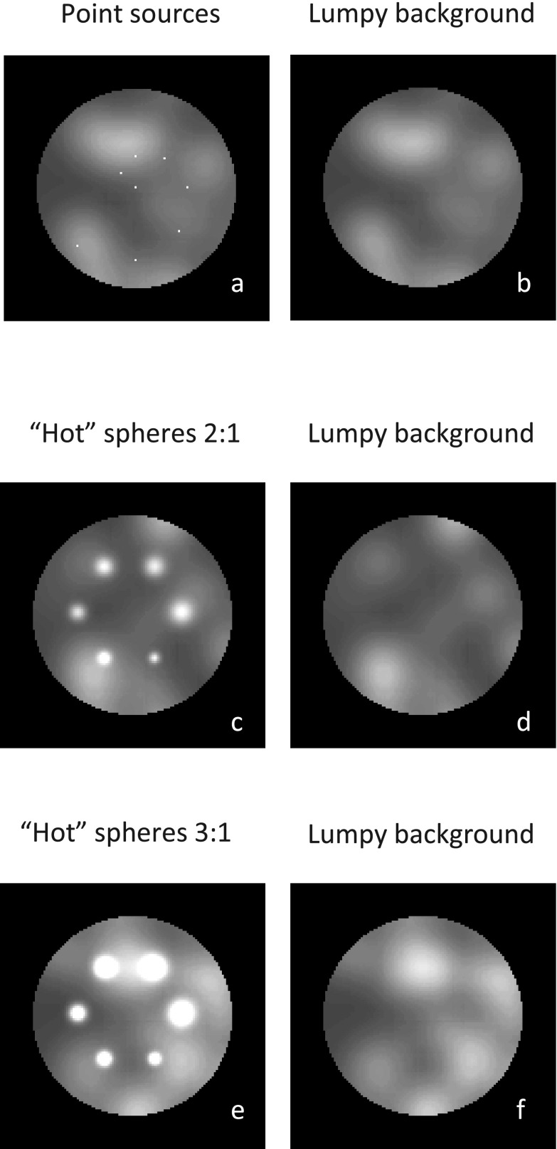
We conducted computer simulations to assess the effect of the second-order regularizer on image spatial resolution, noise performance, and lesion detection, as well as to assess the computational efficiency of PAPA. A lumpy phantom with Gaussian blobs, motivated by a previous study,34 was designed to accomplish the required assessment. A cylinder with diameter 20.8 cm and length 14.1 cm was used as the body of the phantom. The cylinder has random background, obtained by superimposing a fixed uniform background and randomly distributed Gaussian blobs, thereby producing a lumpy background. Specifically, the lumpy background was modeled by
| (9) |
where Gauss(h, σ, pk) represents a 3D Gaussian blob with standard deviation σ and maximum activity h centered at the kth random point source pk, and K is a Poisson variable. We randomly selected K point sources in the cylinder and applied the Gaussian function accordingly. We then added these broadened sources to a uniform cylinder to generate the lumpy background. We chose K = 50, h = 6 MBq/cm3 (which is half of the averaged total background activity), and σ = 30 mm. Two well-separated transaxial planes, each with six 3D Gaussian spheres (whose σ varied over the range 4–9 mm), were placed within the lumpy background. The spheres, all with the same maximum activity, were Gaussian-blurred. The ratio of maximum activity to mean background was 3:1 and 2:1 for the first and second sets (planes) of spheres, respectively [Figs. 1(c) and 1(e)]. To characterize the reconstructed image spatial resolution, we introduced a third transaxial plane containing eight point (i.e., small) sources into the cylinder [Fig. 1(a)]. Their sizes were 2.2 × 2.2 × 2.2mm3 and their activity-to-mean-background ratio was 100:1. Under such conditions, the point sources represent background perturbations, as has been discussed in Rahmim and Tang35 and Wilson.36 Finally, for the local point spread function (LPSF) estimation and lesion detectability comparison, we generated a reference cylinder with the same lumpy background activity, but without the hot Gaussian spheres or point sources [Figs. 1(b), 1(d) and 1(f)].
FIG. 1.
Transaxial cross sections through phantom containing: (a) and (b) background with and without eight point sources; (c) and (d) background with and without six Gaussian spheres (σ = 4–9 mm) with maximum-activity-to-mean-background ratio of 2:1; (e) and (f) same as in c and d, but with a different slice of lumpy background, and with ratio increased to 3:1.
2.D.2. Simulated SPECT data
We used the Monte Carlo simulation software package, SIMIND,37 to obtain fan-beam (focal length 43.1 cm) Tc-99m SPECT data for the phantom with Gaussian spheres and point sources and the reference phantom. All the simulated objects were made of water. The simulation for each phantom consisted of 120 projection views in a 128 × 64-dimensional detector matrix with 3.56 × 3.56mm2 detector elements, and reconstruction space voxel size 2.2 × 2.2 × 2.2mm3. We note that fan-beam collimators are used exclusively in brain SPECT studies. During data acquisition, the radius of rotation (ROR) for the gamma camera was set to 13.0 cm. We used an 18% energy window centered at 140 keV. Only primary photons and first-order scattered photons within this energy window were considered. We simulated a total of 9.8 × 10⁸ photon histories in order to suppress photon-flux fluctuations. The Monte Carlo-simulated projection images so obtained were multiplied by an appropriate constant to reach a total of 8.4 × 10⁶ counts in 120 views. This total corresponds to an average of 7 × 10⁴ counts per projection view. The total volume of the simulated phantom was 4726 cm3, whereas human brain volume generally does not exceed 1500 cm3.38 Therefore, we expect that it would correspond to 2.8 × 10⁶ counts in 120 views (2.3 × 10⁴ counts per projection view) for a brain with similar mean specific activity. This count level corresponds roughly to 50% of a typical administered dose, because the recommended total number of counts in brain SPECT is 5.0 × 10⁶ or more.39 Based on these near noiseless projection data, we used a Poisson random number generator to create 100 noise realizations for each phantom.
2.E. Reconstruction methods
In the current numerical study, we compare the following four competing reconstruction methods:
2.E.1. ML GPF-EM
The widely used reconstruction method in SPECT clinical imaging OSEM (Ref. 40) is the ordered-subset version of the ML-EM (Ref. 8) algorithm. The ML-EM attempts to find the most likely image given the data, i.e., the image that maximizes the likelihood of producing the acquired projection data. For Poisson data (1), it leads to the following optimization model:8
| (10) |
The ML-EM algorithm has the following form:
where k is the iteration number.
It is well-known that with increasing iteration number for unconstrained ML-EM, the spatial resolution of reconstructed images increases accompanied by noise increase. The common solution to regularize the reconstructed images is to stop the algorithm at a predetermined iteration number and remove excessive noise by a postsmoothing filter. We note that stopping iterations too early might lead to wrong solutions. Therefore, one needs to experimentally determine the stopping rule for the specific imaging problem. Based on our experiments, we stopped ML-EM at the 100th iteration and applied a 3D Gaussian postsmoothing filter to the obtained image volume.
2.E.2. TV-OSL
The Panin–Zeng–Gullberg TV-OSL method13 is a penalized likelihood (PL) reconstruction algorithm which incorporates a smoothed TV norm in the objective function of Eq. (10). The smoothed TV increases as image noise increases, thus increasing the objective function, which has the effect of steering the optimization algorithm away from noisier images. This reconstruction method includes a small ad hoc positive parameter ε to avoid nondifferentiability of the TV norm and the resultant PL optimization model reads
| (11) |
where is a smoothed version of the TV norm. The OSL iterative scheme11 can be implemented with the differentiable regularizer R,
We note that in the OSL approach, the regularizer is added in the denominator of the sensitivity term. The convergence is not ensured and such an algorithm is only successful for small penalty-weight λ. When λ vanishes, the TV-OSL method reduces to the ML-EM algorithm. We stop the TV-OSL iterative procedure at the 100th iteration. We remark that since TV-OSL is based on a first-order TV regularizer, it will create staircase artifacts.
2.E.3. PAPA with total variation regularizer (TV-PAPA)
As mentioned in Sec. 2.B, the TV penalty function can be formulated as the composition of a convex nonnegative function φ1 and a first-order gradient operator B1. Thus, given Poisson-distributed projection data, the TV-penalized likelihood optimization model reads
| (12) |
Since the convex function φ1 that defines the TV norm is nondifferentiable, traditional gradient-type and expectation maximization-type algorithms, which require the availability of gradient of the penalty function, cannot solve optimization problem (12). Our previously developed TV-PAPA method22 does not require any kind of smoothing technique (e.g., introduction of ad hoc parameters as has been done in the TV-OSL method) to deal with nondifferentiability, and can iteratively solve problem (12) based on its fixed-point characterization. Indeed, given any initial , for any k = 0, 1, …, the TV-PAPA iterative scheme reads
In the above scheme, b ∈ ℝ3d is the dual variable in gradient domain, S is the d × d diagonal, positive-definite, preconditioning matrix, and μ is a positive parameter. Following our previous work,17 we choose S as the diagonal matrix at the kth iteration (Sec. 2.C). We emphasize that in contrast with the TV-OSL method, all PAPA-type methods are guaranteed to converge. We expect that because TV-PAPA utilizes a first-order TV regularizer, therefore it will produce staircase artifacts. We stop the TV-PAPA iterative procedure at the 100th iteration.
2.E.4. HOTV-PAPA
Recalling the formulation of second-order TV regularizer (4), the goal behind the proposed HOTV-PAPA method is to solve the following penalized likelihood optimization problem:
| (13) |
Since model (13) incorporates second-order derivatives into its penalty function, it can better suppress the reconstructed image noise with reduced staircase artifacts, as compared to first-order TV regularization models. It is also guaranteed to converge. We stop the HOTV-PAPA iterative procedure at the 100th iteration.
2.F. Image degradation compensation
We applied distance-dependent resolution modeling and attenuation compensation in the reconstructions. Because the comparisons in this study were made within the same simulation framework, a simple scatter model was used. Only the first-order scatter present in the simulated SPECT data was corrected by using the broad-beam attenuation coefficient μ = 0.12 cm−1 at 140 keV.
2.G. Parameters
The optimal values of penalty-weight λ for competing methods were obtained by performing sets of trial reconstructions with λ ranging from 10−4 to 1, and by quantitatively analyzing the dependence of spatial resolution and image noise on λ. Spatial resolution was assessed by calculating the full width at half maximum (FWHM) of the local PSFs obtained for the mean images of the reconstructed point sources at various locations with mean reference background subtracted. We qualitatively (visually) balanced the trade-off between spatial resolution and image noise in the difference images (hot spheres phantom with reference background subtracted).
Because HOTV-PAPA required estimation of four parameters: λ1, λ2 and μ1, μ2, we set and at the kth iteration.22 We kept λ1 equal to the λ used in TV-PAPA, and chose λ2 by balancing resolution and the severity of staircase artifacts. This was performed by increasing λ2 until the artifacts disappeared while avoiding unacceptable resolution loss. For GPF-EM, we chose the standard deviation (radius) of the Gaussian blurring kernel to be 2.9 mm to approximately match the local spatial resolution of HOTV-PAPA reconstruction.
2.H. Quantification of reconstruction
Because of the effects of detector response, photon attenuation, and scatter, SPECT (and PET) imaging systems are nonlinear and shift-variant, and have nonstationary noise properties. Therefore, one needs to carefully select metrics suitable for such systems.35,36,41 In the analysis of our results, we focused on the LPSF, noise performance [including ensemble noise, ensemble voxel variance, true variance of background voxels, and local noise power spectrum (LNPS)], and on lesion detectability. We also used the mean square error (MSE) to quantify the overall reconstruction error level.
2.H.1. Local point spread function
Following the well-established methods,35,36,41 we introduced a number of point sources located in the same transaxial cross section of the cylinder, but at different radial distances from its central axis as a perturbation to the background (i.e., target absent) object. We assumed that the reconstruction operation on such objects was approximately linear. After reconstruction of the perturbed image, the reconstruction of noiseless lumpy background projection data was subtracted to provide the LPSF. Then, the FWHMs of LPSFs were calculated, thereby providing an estimate of the local spatial resolution for each SPECT reconstruction method.
2.H.2. Ensemble noise and image roughness
Ensemble noise provides a useful metric of noise across independent realizations, because it is inversely proportional to detection-task performance. For the kth region of interest ROIk (k = 1, 2, …, K and K is the total number of background ROIs), the ensemble noise is defined as the variance of ROI mean activities mr,k across multiple noise realizations r = 1, 2, …, R,35,41
| (14) |
where is the average of mean activities in ROIk over R noise realizations and is defined for each ROIk. We can further average this statistic over the K background ROIs to generate the final ensemble noise metric .
As is pointed out by Rahmim and Tang,35 the use of a simple dual-metric (e.g., resolution vs image noise) trade-off to predict lesion-detection task performance is flawed, especially when image roughness is used. Utilization of the ensemble noise (), defined above, is more appropriate than that of image roughness (), which is defined for a single noise realization as
| (15) |
where fi is the reconstructed activity for voxel i in a ROI consisting of N voxels with mean activity m.
According to Rahmim and Tang [Eq. (22)],35 the expectation of can be written as
| (16) |
where for a uniform background region, is the true variance of background voxels and covi,j is the intervoxel covariance, is ensemble averaged ith voxel value, and is the mean activity in the ROI averaged over all noise realizations. The last term in Eq. (16) represents noise-free image roughness (nonuniformity). Therefore, by calculating using the difference image, one can eliminate the bias due to the noise-free image nonuniformities. The difference image is obtained by subtraction of the reference background. Further, the use of large N allows neglecting the second term in comparison with the first, thus permitting reasonable estimation of from one noise realization.
2.H.3. Ensemble voxel variance
Ensemble voxel variance35,41 is defined for a given voxel i with respect to multiple noise realizations r = 1, …, R as
| (17) |
where fir is the reconstructed activity for voxel i at noise realization r, R is the number of noise realizations, and is the average activity of voxel i over realizations. The above definition is for a single voxel and hence a variance image can be generated.
2.H.4. LNPS
We characterized the noise performance by means of the normalized LNPS. The LNPS has been used to evaluate background noise properties in SPECT (Refs. 36 and 42) and PET (Ref. 35) iterative reconstruction methods, as well as in the context of CT reconstruction.43,44 A ROI (a square of size 32 voxels by 32 voxels) in the center of a transaxial cross section of the reconstructed reference cylinder was used.
2.H.5. Detectability of hot Gaussian spheres
We applied the channelized Hotelling observer (CHO)45,46 to quantify the detectability of the hot Gaussian spheres. We used five nonoverlapping and rotationally symmetric channels with the following pass-bands: [0.016, 0.031], [0.031, 0.063], [0.063, 0.125], [0.125, 0.250], and [0.250, 0.500] cycles/pixel, following the published approaches.47,48 No internal observer noise was modeled. A total of 800 noise realizations were used: 400 for the reference lumpy cylinder (i.e., target absent) and 400 for the cylinder with Gaussian spheres and point sources. We used half of the simulated data to estimate the observer vectors (oCHO). The results were then applied to the other half of the data to obtain the Hotelling-observer detectability indices (dCHO).
2.H.6. Mean square error
The MSE is a global image quality metric. It quantifies the difference between the activity reconstruction f and the phantom (the ground truth activity) fO in the whole object. It is defined by
| (18) |
where fi and fOi are voxel activities in the reconstructed image and phantom, respectively, and N is the total number of voxels in the reconstruction space.
3. RESULTS
3.A. Reconstructed images
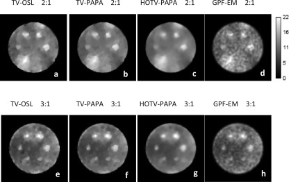
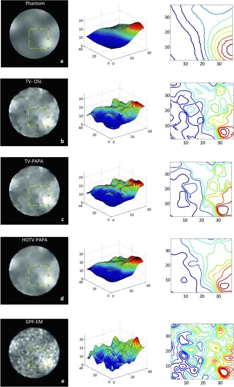
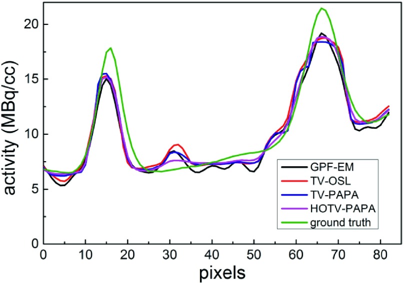
Figures 2, 3, and 5 show examples, respectively, of point sources, Gaussian spheres, and lumpy backgrounds reconstructed using the four competing methods with optimal penalty-weights for the same noise realization of the simulated SPECT data. In Fig. 3, we show two sets of reconstructed Gaussian spheres with maximum-activity-to-mean-background ratio of 3:1 and 2:1. Horizontal line profiles through the centers of reconstructed images [Figs. 3(e)–3(h)] and ground truth [Fig. 1(c)] are shown in Fig. 4. We observe that the activities of reconstructed lesions are similar for all four methods, while the noise-related fluctuation patterns are quite different. Staircase artifacts are evident in both TV-OSL and TV-PAPA reconstructions [Figs. 3(a), 3(b), 3(e), and 3(f)]. HOTV-PAPA, though, greatly reduces such artifacts [Figs. 3(c) and 3(g)]. Similar phenomena are observed in the reconstructed lumpy backgrounds (Fig. 5). To better visualize these artifacts, in Fig. 5, we also present surface plots, with corresponding contours. We observe that the presence of staircasing artifacts in TV-OSL and TV-PAPA reconstructions leads to creation of a few closed contours not present in the noise-free phantom images. They are mostly eliminated in contour plots for HOTV-PAPA. The GPF-EM produces a high number of closed contours. A qualitative comparison of images and surface plots confirms the superiority of HOTV-PAPA over the other three methods, with respect to suppression of image noise and staircase artifacts.
FIG. 2.
Transaxial cross sections through the reconstructed volumes containing point sources using (a) TV-OSL; (b) TV-PAPA; (c) HOTV-PAPA; and (d) GPF-EM. The images were obtained at 100 iterations.
FIG. 3.
Transaxial cross sections through volumes containing Gaussian spheres, reconstructed using TV-OSL (a) and (e); TV-PAPA (b) and (f); HOTV-PAPA (c) and (g); and GPF-EM (d) and (h). Images in the upper and lower rows correspond, respectively, to phantom transaxial cross sections with hot spheres with maximum-activity-to-mean-background ratio of 2:1 [Fig. 1(c)] and 3:1 [Fig. 1(e)]. The images were obtained at 100 iterations.
FIG. 5.
Transaxial cross sections through reconstructed volumes containing only lumpy background with corresponding surface plots and contour plots of (a) phantom; (b) TV-OSL; (c) TV-PAPA; (d) HOTV-PAPA; and (e) GPF-EM. In the surface plots, the z-axis represents activity level in the unit of MBq/cm3. In the contour plots, the activity isolines of the same color correspond to same absolute activity level. The images were obtained at the 100th iteration for one noise realization.
FIG. 4.
Horizontal line profiles through centers of reconstructed images [Figs. 3(e)–3(h)] and ground truth [Fig. 1(c)]. Peaks at pixels 17 and 68 represent centers of Gaussian spheres with FWHM values 21.1 and 14.1 mm, respectively.
3.B. Numerical analysis
3.B.1. Local spatial resolution
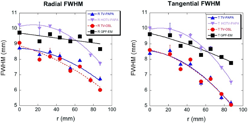
The local spatial resolution was estimated by calculating the FWHM of the LPSF obtained for the mean images of the reconstructed point sources at various radial locations with the mean reference background subtracted (not shown). It was obtained by least-squares fitting of a Gaussian function plus constant background to line profiles through the point source images in the radial and tangential directions (Fig. 6). We observe that tangential FWHM is always smaller than radial FWHM, and that they decrease monotonically with increasing radial distance from the isocenter. Similar behavior was reported for the ordered subsets expectation maximization reconstruction of SPECT data.49 The radial dependence of the FWHM of LPSFs for GPF-EM is best fitted by a linear function, while the other methods require quadratic functions. The local spatial resolution of TV-PAPA is similar to that of TV-OSL and better than that observed for HOTV-PAPA. The mean FWHM of LPSF for HOTV-PAPA and GPF-EM is comparable due to our selection, the Gaussian blurring kernel radius at σ = 2.9 mm.
FIG. 6.
The radial (left panel) and tangential (right panel) FWHM of LPSFs obtained for TV-PAPA, HOTV-PAPA, TV-OSL, and GPF-EM with optimized penalty-weights λ1 = λ = 0.018, λ2 = 0.007, and the Gaussian blurring kernel radius σ = 2.9 mm for GPF-EM. Error bars represent the asymptotic standard parameter errors expected in the least-squares fitting of the FWHM. Solid lines correspond to linear fits for GPF-EM and second-order polynomial fits for TV-PAPA, HOTV-PAPA, and TV-OSL.
3.B.2. Mean square error
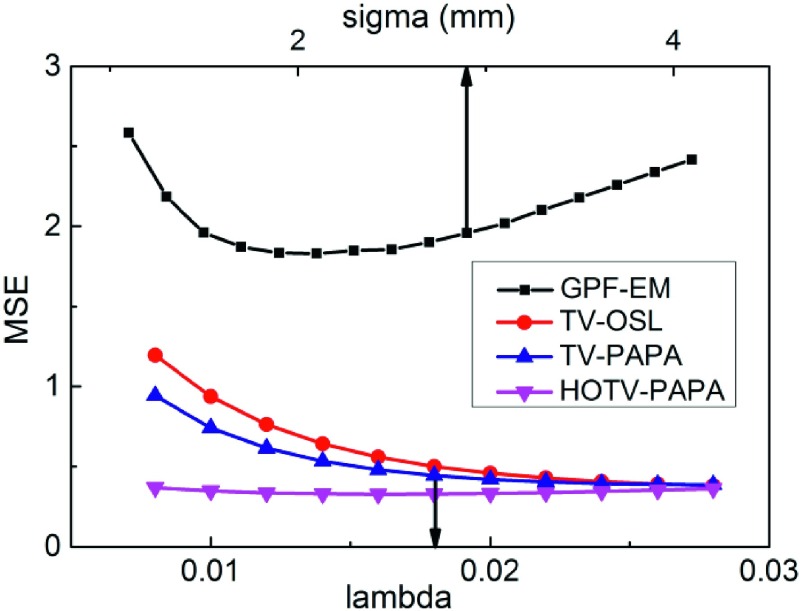
The MSE (18) plots for the images reconstructed using the four reconstruction methods are shown in Fig. 7. Although MSE has some disadvantages as an image quality metric (e.g., sensitivity to displacement and insensitivity to noise-resolution trade-off), it estimates well the reconstruction accuracy. The results show that regardless of reconstruction parameters, HOTV-PAPA and TV-PAPA consistently produce smaller MSE than GPF-EM, as well as TV-OSL with the same penalty-weight.
FIG. 7.
MSE (18) vs postreconstruction Gaussian filter radius σ for GPF-EM and vs penalty-weight λ for TV-OSL and TV-PAPA, and λ1 for HOTV-PAPA reconstructions. We arrived at the same penalty-weight value for TV-PAPA, HOTV-PAPA, and TV-OSL (λ = λ1 = 0.018). Second penalty-weight, λ2, for HOTV-PAPA reconstructions was set const (λ2 = 0.007) for the whole range of λ1. The arrow pointing at the lower axis indicates the value of penalty-weight that was selected for reconstructions in the present comparative studies. The nonoptimal Gaussian blurring kernel radius σ = 2.9 mm (upper arrow) was selected to approximately match the local spatial resolution between GPF-EM and HOTV-PAPA.
3.B.3. Image noise performance
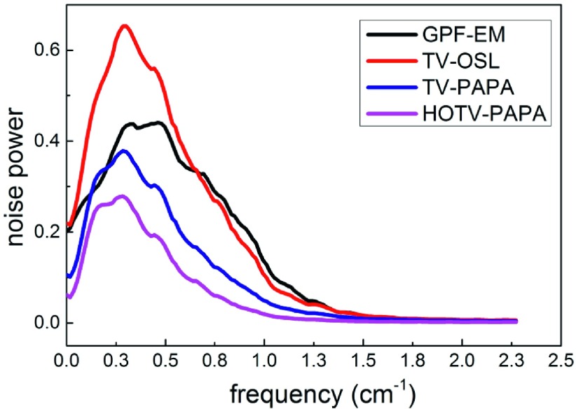
Figure 8 shows LNPS images obtained for HOTV-PAPA and the other three methods for one location close to the phantom center. The mean radial profiles through the LNPS images are shown in Fig. 9. We observe large differences with respect to LNPS. First, LNPS for HOTV-PAPA has the lowest mean and maximum amplitudes followed by TV-PAPA, GPF-EM, and TV-OSL. Second, TV-OSL, TV-PAPA, and HOTV-PAPA suppress high-frequency noise spectra components better than GPF-EM. Although TV-PAPA and TV-OSL are minimizing almost identical objective functions, TV-PAPA provides much better noise suppression than TV-OSL does (Table I).
FIG. 8.
Localized noise power spectra for (a) TV-OSL; (b) TV-PAPA; (c) HOTV-PAPA; and (d) GPF-EM.
FIG. 9.
Averaged radial profiles through the local noise power spectra obtained for the four methods. Radial profiles were selected every 10°. A total of 18 profiles were used for averaging.
TABLE I.
Mean and maximum amplitudes, and mean spatial frequencies corresponding to maxima in LNPS amplitudes for spectra obtained using the four methods.
| Method | GPF-EM | TV-OSL | TV-PAPA | HOTV-PAPA |
|---|---|---|---|---|
| Average LNPS amplitude (arbitrary units) | 0.28 | 0.31 | 0.16 | 0.10 |
| Maximum LNPS amplitude (arbitrary units) | 0.66 | 0.43 | 0.38 | 0.28 |
| Spatial frequency corresponding to maximum LNPS amplitude (cm−1) | 0.51 | 0.34 | 0.33 | 0.32 |
3.B.4. Ensemble noise
The calculated ensemble noise is shown in Fig. 10. It was calculated using 24 ROIs and 100 noise realizations; 12 ROIs are centered at slice 23, and the other 12 are centered at slice 43. We note that slices 23 and 43 are central cross sections for the two layers of Gaussian spheres, respectively. The radii of the ROIs are 8 voxels. We observe that HOTV-PAPA greatly outperforms all the other methods, followed by TV-PAPA, while TV-OSL and GPF-EM have similar ensemble variances.
FIG. 10.
Ensemble noise, (14), calculated for four competing methods and its standard error.
3.B.5. Image roughness
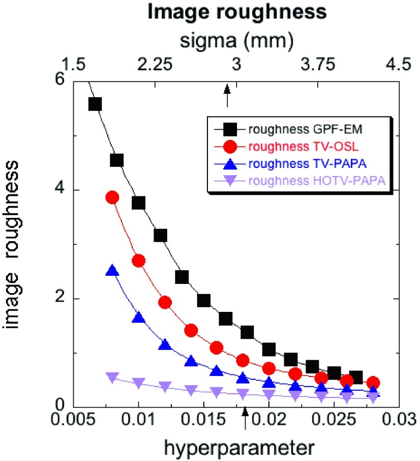
We used the same 24 ROIs as described in Sec. 3.B.4 to calculate (15). In order to account for noise-free image nonuniformity, we calculated on difference images (with reference background subtracted) for one noise realization50 (see Sec. 2.H.2). Because the total number of voxels used in our ROIs was large, such an approach allowed reasonable estimation of the true background voxels variance (16).35 The results are shown in Fig. 11. We observe that the image roughness for the range of parameters investigated is a monotonic function of the penalty-weight. It is the lowest for HOTV-PAPA, followed by TV-PAPA, TV-OSL, and GPF-EM. These results are consistent with ensemble voxel variance estimation (Sec. 3.B.6).
FIG. 11.
Image roughness, (15), calculated on difference images (with reference background subtracted) for one noise realization for four competing methods vs postreconstruction Gaussian filter radius σ for GPF-EM, and vs penalty-weight λ for TV-OSL and TV-PAPA, and λ1 = λ, λ2 = const = 0.007 for HOTV-PAPA reconstructions for the whole range of λ1. The arrow pointing at the lower axis indicates the value of penalty-weight (λ = λ1 = 0.018) that was selected for reconstructions in the present comparative studies. The arrow pointing at the upper axis indicates the selected value of Gaussian postfilter radius, σ = 2.9 mm used in comparative studies of four methods. The solid lines are provided as visual guides.
3.B.6. Ensemble voxel variance
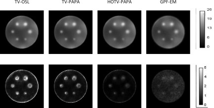
The mean and variance images across 100 different noise realizations are shown in Fig. 12.
FIG. 12.
Upper row: reconstructed mean images of Gaussian spheres with maximum-activity-to-mean-background ratio of 2:1 [Fig. 1(e)]. Lower row: corresponding variance images. All images were obtained by reconstruction of 100 noise realizations for TV-OSL, TV-PAPA, HOTV-PAPA, and GPF-EM at the 100th iteration. The corresponding reconstructed images obtained for one noise realization are shown in Figs. 3(a)–3(d).
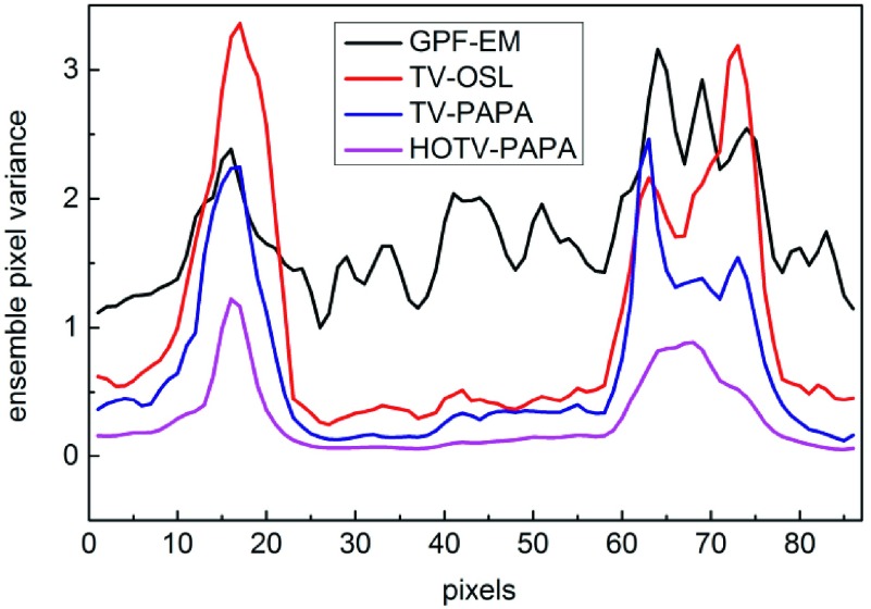
We observe very different appearances of variance images (Fig. 12) for the four methods, as indicated by the line profiles in Fig. 13. The voxel variance has the lowest amplitude for HOTV-PAPA followed by TV-PAPA and TV-OSL. They exhibit low noise levels when away from hot spheres. TV-OSL has the highest amplitude at the hot sphere locations, and GPF-EM produces high ensemble voxel variances across the whole reconstructed image. In the variance images reconstructed with TV-OSL and TV-PAPA, and to a lesser degree with HOTV-PAPA, we observe edge artifacts, appearing as rings, similar to the ones observed for PET reconstructions and discussed in Rahmim and Tang.35 They are practically invisible in the mean images. GPF-EM variance images do not exhibit edge artifacts.
FIG. 13.
Horizontal line profiles through centers of variance images in Fig. 12. Peaks at pixels 17 and 68 correspond to centers of Gaussian spheres with FWHM values 21.1 and 14.1 mm, respectively.
3.B.7. CHO lesion detectability
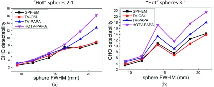
Visual examination of reconstructed images for one noise realization (Fig. 3) indicates that the simulated lesions (hot Gaussian spheres) exhibit higher conspicuity for HOTV-PAPA. This is confirmed by the CHO studies of the reconstructed images. We have found higher CHO detectability indices for HOTV-PAPA, followed by TV-PAPA and GPF-EM/TV-OSL (Fig. 14). We note that GPF-EM and TV-OSL exhibit comparable lesion detectability. HOTV-PAPA is superior to the other methods, because it suppresses Poisson noise better, without creating structural fluctuations, i.e., staircase artifacts. The fluctuations in detectability with respect to lesion sizes [Fig. 14(b)] are probably associated with the lumpy background. We note that the center of the 14 mm sphere at 9 o’clock location is in the region of relatively “cold” background, compared to other spheres [Figs. 1(e) and 1(f)]. As a result, the conspicuity of this sphere is higher than that of 11 and 17 mm spheres located in the same transaxial cross section, resulting in the observed jumps in CHO detectability indices. This is not the case for the set of hot spheres shown in Fig. 1(c), with corresponding background shown in Fig. 1(d).
FIG. 14.
CHO detectability indices of Gaussian spheres of various sizes for two sets of hot spheres: (a) spheres with 2:1 maximum-activity-to-mean-background ratio [Figs. 3(c) and 3(d)] and (b) spheres with 3:1 maximum-activity-to-mean-background ratio [Figs. 3(e) and 3(f)]. The solid lines connecting calculated data points are added as visual aids. The estimated errors are smaller than the symbols.
3.B.8. Convergence speed and computation time
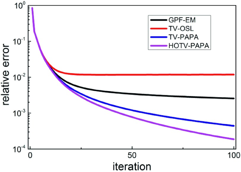
Table II shows the CPU time expended and the number of complete iterations used by GPF-EM, TV-OSL, TV-PAPA, and HOTV-PAPA for reconstruction of our simulated projection data. The relative error we have used is defined as .
TABLE II.
Number of complete iterations and CPU time needed to achieve various relative error levels.a
| GPF-EM | TV-OSL | TV-PAPA | HOTV-PAPA | |||||
|---|---|---|---|---|---|---|---|---|
| Relative error | Iteration | Time (s) | Iteration | Time (s) | Iteration | Time (s) | Iteration | Time (s) |
| 10−1 | 4 | 204 | 4 | 209 | 4 | 249 | 4 | 258 |
| 10−2 | 15 | 732 | — | — | 14 | 677 | 14 | 761 |
| 10−3 | — | — | — | — | 57 | 2850 | 44 | 2114 |
Reconstructions were performed on a workstation with dual Intel Xeon E5-2650 processors.
From Table II, we conclude that, under the same stopping criteria, HOTV-PAPA is better than TV-PAPA and much better than TV-OSL and GPF-EM in terms of the convergence speed. The relative error versus iteration number is shown in Fig. 15. We note that TV-OSL and GPF-EM cannot meet the stopping criteria for the 10−2 and 10−3 tolerance levels, respectively (see entries marked by dashes in Table II). Further, one can perform reconstruction using HOTV-PAPA and TV-PAPA in a reasonable time frame, comparable to that for GPF-EM.
FIG. 15.
Relative error versus iteration number for the four methods.
3.B.9. Comparison of objective function values for TV-OSL and TV-PAPA
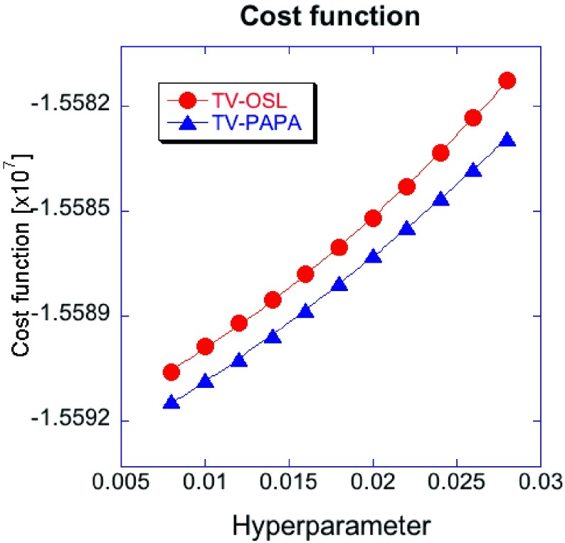
Figure 16 demonstrates that, for the same number of iterations, the value of the objective function for TV-OSL is always larger than for TV-PAPA, independent of the penalty-weight selected. It indicates the superior solution of optimization problem (2) obtained using TV-PAPA, as compared to TV-OSL. This helps to explain the poor performance of TV-OSL in terms of LNPS, detectability of hot Gaussian spheres, and convergence speed, compared to TV-PAPA and HOTV-PAPA.
FIG. 16.
Cost function (2) at 100 iterations vs penalty-weight for TV-OSL and TV-PAPA. Solid lines represent second-order polynomials fitted to the data.
4. DISCUSSION
In the present work, we have investigated the performance of our recently developed PAPA for solving the penalized maximum likelihood optimization model for SPECT reconstruction problem. This algorithm belongs to a novel class of fixed-point proximity methods. We considered the regularization model that has HOTV in the penalty function. We compared the performance of the proposed method to TV-PAPA, one-step-late method with total variation regularizer (TV-OSL), and the clinically used EM algorithm with Gaussian post filter (GPF-EM) radius selected to match LPSF of HOTV-PAPA. We applied these four methods to Monte Carlo-simulated Tc-99m SPECT data generated from two numerical phantoms: a water cylinder with lumpy background containing variously sized hot spheres, each with Gaussian activity distribution, and a reference cylinder with identical lumpy background only. We analyzed the reconstructed images quantitatively and qualitatively and determined that HOTV-PAPA yields superior signal-to-noise ratio in CHO studies.
The images reconstructed using PAPA-type methods—in comparison with TV-OSL and GPF-EM—have lower local noise power spectra mean and maximum amplitudes. The LNPS maxima are shifted toward lower spatial frequencies; thus, we expect better suppression of high frequency noise, compared to GPF-EM.
The reconstructed images also exhibit much lower level of ensemble noise, ensemble voxel variance, image roughness, and the overall voxel variance. HOTV-PAPA performs the best in all these categories. Because the reconstructed lesion activities are similar for all four methods, we have determined that improved lesion detectability by HOTV-PAPA and TV-PAPA stems from superior noise suppression by these methods. While images reconstructed using both TV-PAPA and TV-OSL are degraded by severe staircase artifacts, HOTV-PAPA substantially reduces such artifacts. The local spatial resolution of TV-PAPA is similar to TV-OSL and better than that observed for HOTV-PAPA, but with the same quadratic dependence on the radial distance from isocenter reaching the lowest values at the edge of the phantom, while the LPSF for GPF-EM method exhibits linear dependence. Furthermore, the overall reconstruction error level as measured by MSE is the lowest for HOTV-PAPA with optimized penalty-weights. The proposed method HOTV-PAPA also converges faster than the other three competing methods.
In future studies, we plan to evaluate HOTV-PAPA using clinical data requiring a more rigorous validation process. A necessary step toward this goal is improving some parts of our model, such as the projection scheme and the scatter correction,1,51 and adding additional types of collimation such as parallel hole. Another active area of research will be the optimal selection of penalty-weight values. With the addition of a second penalty-weight, the parameter space grows considerably making the selection process difficult. The adaptation of HOTV-PAPA into the clinic will require development of some form of guidance in the penalty-weight selection, so that clinicians can adapt the images to their own preferences.
5. CONCLUSIONS
In sum, we have shown that both HOTV-PAPA and TV-PAPA greatly outperform the clinical GPF-EM method and the Panin, Zeng, and Gullberg13 TV-OSL method for high-noise simulated SPECT data in terms of hot lesion detectability, noise suppression, and computational efficiency. Unlike TV-PAPA and TV-OSL, HOTV-PAPA avoids substantial staircase artifacts, while producing reconstructed images with higher lesion detectability and reasonable LPSF. Therefore, HOTV-PAPA could provide clinically useful reconstructions of low-dose (hence higher-noise) SPECT data, thus offering a promising approach to the important goal of reducing radiation dose to patients in selected nuclear medicine studies.
ACKNOWLEDGMENTS
This research has been supported in part by the United States National Science Foundation under Grant No. DMS-1115523, by the Guangdong Provincial Government of China through the “Computational Science Innovative Research Team” program, by the Natural Science Foundation of China under Grant Nos. 11071286, 91130009, and 11471013, and by the Promotive Research Fund for Excellent Young Scientists of Shandong Province under Grant No. BS2014DX003. This work has also been supported in part by Award No. 5-28527 from the National Center for Research Resources (NCRR), a component of the National Institutes of Health (NIH) and the NIH Roadmap for Medical Research, and by the Center of Emerging and Innovative Sciences (CEIS), a NYSTAR designated Center for Advanced Technology. In addition, the authors wish to thank Dr. Arman Rahmim for his advice on the design of the study. The content is solely the responsibility of the authors and does not necessarily represent the official views of the National Center for Research Resources or the National Institutes of Health. This work has been supported in part by an award from the Carol M. Baldwin Breast Cancer Research Fund.
REFERENCES
- 1.Wernick M. and Aarsvold J., Emission Tomography: The Fundamentals of PET and SPECT (Academic, Waltham, MA, 2004). [Google Scholar]
- 2.Bolus N. E., “NCRP report 160 and what it means for medical imaging and nuclear medicine,” J. Nucl. Med. Technol. 41, 255–260 (2013). 10.2967/jnmt.113.128728 [DOI] [PubMed] [Google Scholar]
- 3.ACR, SNMMI, ASNC, AAPM, Image wisely, 2015, available at http://www.imagewisely.org/Imaging-Modalities/Nuclear-Medicine.
- 4.Caobelli F., Kaiser S. R., Thackeray J. T., Bengel F. M., Chieregato M., Soffientini A., Pizzocaro C., Savelli G., Galelli M., and Guerra U. P., “IQ SPECT allows a significant reduction in administered dose and acquisition time for myocardial perfusion imaging: Evidence from a phantom study,” J. Nucl. Med. 55, 2064–2070 (2014). 10.2967/jnumed.114.143560 [DOI] [PubMed] [Google Scholar]
- 5.Duvall W. L., Croft L. B., Godiwala T., Ginsberg E., George T., and Henzlova M. J., “Reduced isotope dose with rapid SPECT MPI imaging: Initial experience with a CZT SPECT camera,” J. Nucl. Cardiol. 17, 1009–1014 (2010). 10.1007/s12350-010-9215-5 [DOI] [PubMed] [Google Scholar]
- 6.Einstein A. J., Blankstein R., Andrews H., Fish M., Padgett R., Hayes S. W., Friedman J. D., Qureshi M., Rakotoarivelo H., Slomka P., Nakazato R., Bokhari S., Di Carli M., and Berman D. S., “Comparison of image quality, myocardial perfusion, and left ventricular function between standard imaging and single-injection ultra-low-dose imaging using a high-efficiency SPECT camera: The MILLISIEVERT study,” J. Nucl. Med. 55, 1430–1437 (2014). 10.2967/jnumed.114.138222 [DOI] [PMC free article] [PubMed] [Google Scholar]
- 7.DePuey E. G., Bommireddipalli S., Clark J., Leykekhman A., Thompson L., and Friedman M., “A comparison of the image quality of full-time myocardial perfusion SPECT vs wide beam reconstruction half-time and half-dose SPECT,” J. Nucl. Cardiol. 18, 273–280 (2011). 10.1007/s12350-011-9340-9 [DOI] [PubMed] [Google Scholar]
- 8.Lange K. and Carson R., “EM reconstruction algorithms for emission and transmission tomography,” J. Comput. Assisted Tomogr. 8, 306–316 (1984). [PubMed] [Google Scholar]
- 9.Shepp L. A. and Vardi Y., “Maximum likelihood reconstruction for emission tomography,” IEEE Trans. Med. Imaging 1, 113–122 (1982). 10.1109/TMI.1982.4307558 [DOI] [PubMed] [Google Scholar]
- 10.Geman S. and Geman D., “Stochastic relaxation, Gibbs distributions, and the Bayesian restoration of images,” IEEE Trans. Pattern Anal. Mach. Intell. PAMI-6, 721–741 (1984). 10.1109/TPAMI.1984.4767596 [DOI] [PubMed] [Google Scholar]
- 11.Green P. J., “Bayesian reconstructions from emission tomography data using a modified EM algorithm,” IEEE Trans. Med. Imaging 9, 84–93 (1990). 10.1109/42.52985 [DOI] [PubMed] [Google Scholar]
- 12.Rudin L. I., Osher S., and Fatemi E., “Nonlinear total variation based noise removal algorithms,” Physica D 60, 259–268 (1992). 10.1016/0167-2789(92)90242-F [DOI] [Google Scholar]
- 13.Panin V. Y., Zeng G. L., and Gullberg G. T., “Total variation regulated EM algorithm [SPECT reconstruction],” IEEE Trans. Nucl. Sci. 46, 2202–2210 (1999). 10.1109/23.819305 [DOI] [Google Scholar]
- 14.Sawatzky A., Brune C., Wubbeling F., Kosters T., Schafers K., and Burger M., “Accurate EM-TV algorithm in PET with low SNR,” in Presented at the Nuclear Science Symposium Conference Record, 2008, NSS ’08 (IEEE, 2008). [Google Scholar]
- 15.Jonsson E., Huang S.-c., and Chan T., “Total-variation regularization in positron emission tomography,” CAM Report 98-48 (University of California, Los Angeles, CA,1998). [Google Scholar]
- 16.Bardsley J. M., “An efficient computational method for total variation-penalized Poisson likelihood estimation,” Inverse Probl. Imaging 2, 167–185 (2008). 10.3934/ipi.2008.2.167 [DOI] [Google Scholar]
- 17.Bardsley J. M. and Goldes J., “Regularization parameter selection and an efficient algorithm for total variation-regularized positron emission tomography,” Numer. Algorithms 57, 255–271 (2011). 10.1007/s11075-010-9427-4 [DOI] [Google Scholar]
- 18.Bardsley J. M. and Luttman A., “Total variation-penalized Poisson likelihood estimation for ill-posed problems,” Adv. Comput. Math. 31, 35–59 (2009). 10.1007/s10444-008-9081-8 [DOI] [Google Scholar]
- 19.Bonettini S. and Ruggiero V., “An alternating extragradient method for total variation-based image restoration from Poisson data,” Inverse Probl. 27, 095001 (2011). 10.1088/0266-5611/27/9/095001 [DOI] [Google Scholar]
- 20.Chaux C., Pesquet J.-C., and Pustelnik N., “Nested iterative algorithms for convex constrained image recovery problems,” SIAM J. Imaging Sci. 2, 730–762 (2009). 10.1137/080727749 [DOI] [Google Scholar]
- 21.Sidky E. Y., Jørgensen J. H., and Pan X., “Convex optimization problem prototyping for image reconstruction in computed tomography with the Chambolle–Pock algorithm,” Phys. Med. Biol. 57, 3065–3091 (2012). 10.1088/0031-9155/57/10/3065 [DOI] [PMC free article] [PubMed] [Google Scholar]
- 22.Krol A., Li S., Shen L., and Xu Y., “Preconditioned alternating projection algorithms for maximum a posteriori ECT reconstruction,” Inverse Probl. 28, 115005 (2012). 10.1088/0266-5611/28/11/115005 [DOI] [PMC free article] [PubMed] [Google Scholar]
- 23.Wolfram Research Mathematica version 10.1 ed. (Wolfram Research, Inc., Champaign, IL, 2015). [Google Scholar]
- 24.Barrett H. H. and Myers K. J., Foundations of Image Science (Wiley-Interscience, New York, NY, 2004). [Google Scholar]
- 25.Geman S. and MacClure D., Bayesian Image Analysis: An Application to Single Photon Emission Tomography (American Statistical Association, Alexandria, VA, 1985). [Google Scholar]
- 26.Kullback S. and Leibler R. A., “On information and sufficiency,” Ann. Math. Stat. 22, 79–86 (1951). 10.1214/aoms/1177729694 [DOI] [Google Scholar]
- 27.Benning M., Brune C., Burger M., and Müller J., “Higher-order TV Methods—Enhancement via Bregman iteration,” J. Sci. Comput. 54, 269–310 (2013). 10.1007/s10915-012-9650-3 [DOI] [Google Scholar]
- 28.Bredies K., Kunisch K., and Pock T., “Total generalized variation,” SIAM J. Imaging Sci. 3, 492–526 (2010). 10.1137/090769521 [DOI] [Google Scholar]
- 29.Chan T., Marquina A., and Mulet P., “High-order total variation-based image restoration,” SIAM J. Sci. Comput. 22, 503–514 (2000). 10.1137/S1064827598344169 [DOI] [Google Scholar]
- 30.Micchelli C. A., Shen L., and Xu Y., “Proximity algorithms for image models: Denoising,” Inverse Probl. 27, 045009 (2011). 10.1088/0266-5611/27/4/045009 [DOI] [Google Scholar]
- 31.Setzer S., Steidl G., and Teuber T., “Infimal convolution regularizations with discrete l1-type functionals,” Commun. Math. Sci. 9, 797–827 (2011). 10.4310/CMS.2011.v9.n3.a7 [DOI] [Google Scholar]
- 32.Clinthorne N. H., Pan T. S., Chiao P. C., Rogers W. L., and Stamos J. A., “Preconditioning methods for improved convergence rates in iterative reconstructions,” IEEE Trans. Med. Imaging 12, 78–83 (1993). 10.1109/42.222670 [DOI] [PubMed] [Google Scholar]
- 33.Lange K., Bahn M., and Little R., “A theoretical study of some maximum likelihood algorithms for emission and transmission tomography,” IEEE Trans. Med. Imaging 6, 106–114 (1987). 10.1109/TMI.1987.4307810 [DOI] [PubMed] [Google Scholar]
- 34.Qi J., “Comparison of lesion detection and quantification in MAP reconstruction with Gaussian and non-Gaussian priors,” Int. J. Biomed. Imaging 2006, 1–10. 10.1155/IJBI/2006/87567 [DOI] [PMC free article] [PubMed] [Google Scholar]
- 35.Rahmim A. and Tang J., “Noise propagation in resolution modeled PET imaging and its impact on detectability,” Phys. Med. Biol. 58, 6945–6968 (2013). 10.1088/0031-9155/58/19/6945 [DOI] [PMC free article] [PubMed] [Google Scholar]
- 36.Wilson D. W., “Noise and Resolution Properties of FB and ML-EM Reconstructed SPECT Images,” Ph.D Dissertation, University of North Carolina at Chapel Hill, 1994. [Google Scholar]
- 37.Ljungberg M., Thesimind Monte Carlo Program (IOP Publishing, Bristol, Philadelphia, 1998). [Google Scholar]
- 38.Holloway R. L., Yuan M. S., and Broadfield D. C., The Human Fossil Record: Brain Endocasts: The Paleoneurological Evidence (John Wiley & Sons Publishers, Hoboken, NJ, 2004). [Google Scholar]
- 39.Juni J. E., Waxman A. D., Devous M. D., Tikofsky R. S., Ichise M., Heertum R. L. V., Carretta R. F., and Chen C. C., Society of Nuclear Medicine and Molecular Imaging (SNMMI), Procedure Standards, http://snmmi.files.cms-plus.com/docs/Brain_SPECT_Guideline_2003.pdf. Procedure Guideline for Brain Perfusion SPECT Using 99mTc Radiopharmaceuticals 3.0, Updated July 1, 2009, Accessed July 14, 2015.
- 40.Hudson H. M. and Larkin R. S., “Accelerated image reconstruction using ordered subsets of projection data,” IEEE Trans. Med. Imaging 13, 601–609 (1994). 10.1109/42.363108 [DOI] [PubMed] [Google Scholar]
- 41.Tong S., Alessio A. M., and Kinahan P. E., “Noise and signal properties in PSF-based fully 3D PET image reconstruction: An experimental evaluation,” Phys. Med. Biol. 55, 1453–1473 (2010). 10.1088/0031-9155/55/5/013 [DOI] [PMC free article] [PubMed] [Google Scholar]
- 42.Tsui B. M. W. and Frey E. C., Collimator-Detector Response Compensation in SPECT (Springer, Quantitative Analysis in Nuclear Medicine Imaging, New York, NY, 2006). [Google Scholar]
- 43.Baek J. and Pelc N. J., “The noise power spectrum in CT with direct fan beam reconstruction,” Med. Phys. 37, 2074–2081 (2010). 10.1118/1.3378673 [DOI] [PMC free article] [PubMed] [Google Scholar]
- 44.Choi J., “Measurement of noise power spectra for CT images reconstructed with different kernels,” J. Convergence Inf. Technol. 8, 70–82 (2013). [Google Scholar]
- 45.Barrett H. H., Yao J., Rolland J. P., and Myers K. J., “Model observers for assessment of image quality,” Proc. Natl. Acad. Sci. U. S. A. 90, 9758–9765 (1993). 10.1073/pnas.90.21.9758 [DOI] [PMC free article] [PubMed] [Google Scholar]
- 46.Barrett H. H., Denny J. L., Wagner R. F., and Myers K. J., “Objective assessment of image quality. II. Fisher information, Fourier crosstalk, and figures of merit for task performance,” J. Opt. Soc. Am. A 12, 834–852 (1995). 10.1364/JOSAA.12.000834 [DOI] [PubMed] [Google Scholar]
- 47.Frey E. C., Gilland K. L., and Tsui B. M. W., “Application of task-based measures of image quality to optimization and evaluation of three-dimensional reconstruction-based compensation methods in myocardial perfusion SPECT,” IEEE Trans. Med. Imaging 21, 1040–1050 (2002). 10.1109/TMI.2002.804437 [DOI] [PubMed] [Google Scholar]
- 48.Niu X., Yang Y., King M. A., and Wernick M. N., “Detectability of perfusion defect in five-dimensional gated-dynamic cardiac SPECT images,” Med. Phys. 37, 5102–5112 (2010). 10.1118/1.3481507 [DOI] [PMC free article] [PubMed] [Google Scholar]
- 49.Kappadath S. C., “Effects of voxel size and iterative reconstruction parameters on the spatial resolution of 99mTc SPECT/CT,” J. Appl. Clin. Med. Phys. 12, 3459 (2011). 10.1120/jacmp.v12i4.3459 [DOI] [PMC free article] [PubMed] [Google Scholar]
- 50.Lodge M. A., Rahmim A., and Wahl R. L., “Simultaneous measurement of noise and spatial resolution in PET phantom images,” Phys. Med. Biol. 55, 1069–1081 (2010). 10.1088/0031-9155/55/4/011 [DOI] [PMC free article] [PubMed] [Google Scholar]
- 51.Hutton B. F., Buvat I., and Beekman F. J., “Review and current status of SPECT scatter correction,” Phys. Med. Biol. 56, R85–R112 (2011). 10.1088/0031-9155/56/14/R01 [DOI] [PubMed] [Google Scholar]


