A Benchmark for Methods in Reverse Engineering and Model Discrimination: Problem Formulation and Solutions

Abstract

A benchmark problem is described for the reconstruction and analysis of biochemical networks given sampled experimental data. The growth of the organisms is described in a bioreactor in which one substrate is fed into the reactor with a given feed rate and feed concentration. Measurements for some intracellular components are provided representing a small biochemical network. Problems of reverse engineering, parameter estimation, and identifiability are addressed. The contribution mainly focuses on the problem of model discrimination. If two or more model variants describe the available experimental data, a new experiment must be designed to discriminate between the hypothetical models. For the problem presented, the feed rate and feed concentration of a bioreactor system are available as control inputs. To verify calculated input profiles an interactive Web site (http://www.sysbio.de/projects/benchmark/) is provided. Several solutions based on linear and nonlinear models are discussed.

The analysis of metabolic and regulatory pathways with mathematical models contributes to a better understanding of the behavior of metabolic processes (Kitano 2000). The setup of the structure of the model, that is, the stoichiometry of the biochemical reaction network, is mainly based on data from database systems or from literature. Recent efforts in measurement technologies like cDNA array data or 2D-gel electrophoresis (Ideker et al. 2001) will enable researchers to produce time courses of several substances from inside the cell. Given such data, a challenging task is to identify the underlying structure of the network (“reverse engineering”) and—if two or more model structures are suited to describe the experimental data—to design new experiments that will allow discrimination between the model candidates. Further problems include identifiability of the model parameters, sensitivity of the parameters, and metabolic design (Stelling et al. 2001).

The main focus of work in the field of reverse engineering lies on the identification of genetic networks, that is, in which way transcription factors are connected to the respective genes. The methods used are based on a steady-state description (Tegner et al. 2003) or on Boolean networks (D'haesseleer et al. 2000; Repsilber et al. 2002). Using time-lagged-correlation matrices (Arkin and Ross 1995; Arkin et al. 1997) or genetic programming techniques (Koza et al. 2001), networks could also be reconstructed if time courses of selected state variables were available.

In contrast to the top-down approach represented by the reverse engineering techniques, the bottom-up approach starts with a mathematical model for genetic and metabolic networks based either on biochemical data from databases or on “cartoons” from literature. One major problem here is the estimation of uncertain or even unknown kinetic parameters, that is, the problem of parameter identification, that covers several tasks. (1) Identifiability: Simply speaking, identifiability is concerned with the following question. Given a particular model for a system and an input-output experiment, is it possible to uniquely determine the model parameters (Faller et al. 2003; Zak et al. 2003)? (2) Parameter estimation: Using optimization methods, a set of parameters is determined in such a way that the difference between the experimentally measured output and the predictive output of the mathematical model becomes minimal (Moles et al. 2003). (3) Finally, the accuracy of the parameters has to be calculated. This is normally done by determining the confidence limits of the estimated parameters (Faller et al. 2003; Swameye et al. 2003). To apply statistical methods for this purpose, a large amount of data is required. On the other hand, using the Fisher-Information-Matrix (see below), only a lower bound for the variances of the parameters can be obtained (Ljung 1999; Banga et al. 2002). This lower bound would be reached if the model equations were linear in the parameters, which is normally not the case. To overcome both problems, an alternative method, the bootstrap method (Press et al. 2002), could be applied.

If two or more model variants are available describing the same experimental observations, methods are available to design new experiments that allow us to discriminate between the variants. Early approaches are described in the literature (e.g., Box and Hill 1967; Munack 1992; Cooney and McDonald 1995). The key idea is to find an input profile that maximizes the difference of the outputs of the competing models. In a series of papers, Asprey and coworkers have developed methods to maximize the outputs of the system (Asprey and Macchietto 2000; Chen and Asprey 2003). This is achieved by using an extended weighting matrix including the variances of the measured state variables and the variances and the sensitivities of the parameters. In Chen and Asprey (2003), several methods for model discrimination are also reviewed.

Here, in silico experimental data for an organism growing in a chemostat as shown in Figure 1 are presented. For this purpose, a computer model was set up based on a fictive network structure. Parameters are chosen in such a way that a realistic behavior could be observed. After reaching a steady state, the flow rates q_in, q_out as well as the concentration of the substrate in the feed c_in are changed. Measurements are available for three metabolites, M1, M2, and M3, representing a small biochemical network of the organism, and for biomass B and substrate S. Because different algorithms for parameter estimation are already described in the literature (Moles et al. 2003), this contribution focuses on the accuracy of the parameters by comparing two methods for determining the variance of the parameters.

Figure 1.

Scheme of the bioreactor. Inputs are flow rates q_in, q_out, and feed concentration c_in. Biomass is assumed to be homogeneously distributed in the reactor. The structure of the biochemical reaction network is unknown and must be identified.

In the next section several problems are formulated to apply strategies in the field of reverse engineering and model discrimination. This paper focuses on different methods for model discrimination. For this purpose, two model variants are set up and parameters are estimated. The paper is written for the interested biological researcher and represents possibilities based on a system-theoretical approach. It will be shown that for the given problem it is not necessary to construct several mutant strains, which is often a time-consuming task, but instead, the application of system-theoretical methods using only control inputs available for a bioreactor system is sufficient to provide satisfactory results. Applications for these methods can be found frequently in the field of molecular and cell biology. Considering signal transduction pathways, open questions concern the mechanism of action of the stimulus, cross-talk phenomena, that is, the interaction of separated signal transduction units, and type of control, for example, control of activity or of synthesis of the components involved. Further applications are concerned with the choice of the correct kinetic description for a biochemical reaction (Asprey and Macchietto 2000) or with the distribution of metabolic fluxes in complex networks (Kremling et al. 2001).

METHODS

Benchmark Problem

Problem Formulation

Based on the measurement of components (intra- and extracellular) or expression data, the network structure has to be identified, that is, the interconnections between the given components have to be detected.

If two or more model variants can describe the available experimental data, the design of a new experiment is required to select the most feasible model structure. For larger submodels for cellular systems, measurements are not available for all state variables. Moreover, the development of new measurement techniques is very time consuming. Hence, strategies that require a lesser number of state variables to be measured and moreover strategies that identify these state variables are advantageous. To design a new experiment, inputs and outputs must be chosen in such a way that parameters can be identified. Furthermore, parameters can only be estimated with high accuracy if the control inputs direct them into sensitive regions.

The problem could also be used as a study in metabolic modeling for students to illustrate methods in model setup, model analysis, and experimental design.

Starting Conditions and Data Generation

Figure 2 shows time courses of metabolite concentrations M1, M2, and M3 as well as the time courses of biomass concentration B and substrate concentration S. The conditions during the chemostat experiment are summarized in Table 1. The molar mass for the substrate used is 342.3 g/mol. The initial conditions for biomass and substrate are 0.1 g/L and 2.0 g/L, respectively. The volume of the bioreactor was held constant at 1.0 L for the given time series (the maximal working volume of the reactor is V_max = 5.0 L).

Figure 2.

Time series data for biomass and substrate (upper left), for substance M1 (upper right), for substance M2 (lower left), and for substance M3 (lower right). Data were generated as described above. Numerical values of the data are given in the Appendix and can be downloaded from the Web site given in the problem formulation.

Table 1.

Conditions During Continuous Culture Experiment

Time	Input
0-20h	qin = 0.25 L/h
	qout = 0.25 L/h
	cin = 2.0 g/L
20-30h	qin = 0.35 L/h
	qout = 0.35 L/h
	cin = 2.0 g/L
30-60h	qin = 0.35 L/h
	qout = 0.35 L/h
	cin = 0.50 g/L

The volume of the bioreactor was held constant at 1.0 L.

Measurements are sampled every 2 h. To allow realistically complex behavior, the following procedure was used. A set of kinetic parameters was chosen for the (hidden) network. “Experimental data” (time profiles of substrate, biomass, and metabolites) were generated by simulation of this hidden network with the abovementioned initial conditions. With a random number rand, the absolute values of the state variables x were modified according to x̂ = x(1 + rand), where rand is normally distributed with mean value m̄ = 0, and the standard deviation σ = 0.1.

With the information given so far, the problem of network identification can be solved.

For the problem of model discrimination, the following additional information can be used.

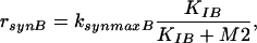
• Metabolite M1 is the first substance synthesized after uptake. The transport mechanism was identified as a Michaelis-Menten reaction law with the parameters given in Table 2.

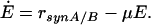
• Substance M3 acts as an enzyme (E) converting metabolite M1 to M2. The reaction is irreversible, and the affinity (dissociation constant) of M1 was determined (Table 2).

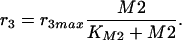
• Degradation of M2 is also identified as a Michaelis-Menten reaction law with the parameters given in Table 2. It is assumed that flux from M2 is responsible for the entire biomass: M2 → biomass.

• The enzyme is subject to control (control of activity or control of synthesis).

Table 2.

Kinetic Parameters for Synthesis of M1, Degradation of M2, and the Affinity of M1 to Enzyme E

Synthesis of M1 Values	rmax = 2.4 × 104 μmol/gDW h
	K = 0.4437 μmol/gDW
Affinity M1 - E Value	K = 12.2 μmol/gDW
Degradation of M2 Values	rmax = 3 × 106 μmol/gDW h
	K = 10.0 μmol/gDW

To verify calculated input profiles an interactive Web site (http://www.sysbio.de/projects/benchmark/) is provided. The site offers the possibility to enter a vector of time points and corresponding values for the input profiles for q_in, q_out, and c_in as well as sampling time points (in h). Initial conditions for all state variables must also be given. Outputs are the time vector at the given sampling time points and a vector of all state variables with added random noise. The time series data are shown in several plots and can also be downloaded.

Model Formulation

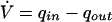
Based on the information given above, equations are set up for the state variables. The equations for reactor volume, entire biomass concentration, and substrate concentration are formulated in a very general way:

1

2

3

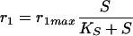
where Mw is the molar mass of the substrate and r₁ is the uptake rate. A Michaelis-Menten kinetic rate law is used:

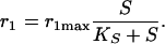4

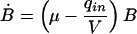
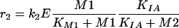
Based on the information given above, two possible model variants are formulated: Model A describes the conversion of M1 to M2 with a noncompetitive inhibition of the enzyme by M2:

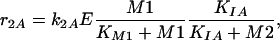5

where k₂ is the turnover number and K_IA the unknown affinity of the inhibitor M2 to the enzyme. Degradation of metabolite M2 is also described with a Michaelis-Menten kinetic rate law:

6

Finally, enzyme synthesis is taken into account with a constant velocity:

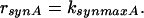7

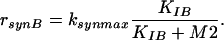
In Model B, the control of enzyme synthesis instead of the control of enzyme activity is considered. Hence, equations 5 and 7 have to be modified. Now, for the enzymatic conversion of M1, a Michaelis-Menten kinetic rate law is assumed. For the enzyme synthesis, a formal kinetic rate law representing an inhibition is used:

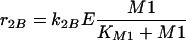8

9

where K_IB represents inhibition of enzyme synthesis by M2.

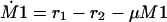
The following system of equations for the concentrations M1, M2, and E is obtained for both models:

10

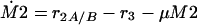11

12

The equations for the intracellular components also consider the dilution by growth represented by the specific growth rate μ. To describe the growth rate, it is assumed that part of the substrate taken up by the organisms is converted into biomass with a yield coefficient Y_xsThe equation for μ is:

13

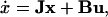
With the vector of state variables x = [B, S, M1, M2, E], the vector of inputs u = [q_in, q_out, c_in], and the vector of model parameters p, the model can now be written in the general form:

14

RESULTS

Estimation of Parameters and Confidence Intervals

Based on the experimental data and the given parameters, the following parameters have to be identified: Y_xs, k_2A/B, k_synmaxA/B, K_IA, and K_IB.

Parameter Estimation

Using a least-squares approach, the parameters should minimize the quadratic error between the simulations and the measured data. As the latter is only available at discrete time points 𝒯 = {t₁, t₂,..., t_N}, the errors at each measurement time point are summed. The squared error is furthermore normalized by the standard deviation of the corresponding measurement noise σ_i and by the maximal measurement. Thus, less noisy signals are more weighted, and all measurements are brought to the same scale. This results in the following objective function that the optimal parameters should minimize:

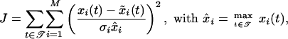15

where M is the number of states, x_i are the measured state variables, and x̃_i the state variables of the models. The standard deviation of the noise is equal for all measurements, that is, σ_i = 0.1x_i. Table 3 shows the resulting parameter values p_opt after a fit with the given experimental data. As the values of the objective functions attained for Model A and Model B differ only slightly, it is not clear which one of the models is better suited to fitting the benchmark problem.

Table 3.

Identified Parameters of Both Models, Attained by Minimizing the Objective Function (15) Over the Benchmark Experiment

Parameter	Model A	Model B
YX/S	6.968 × 10−5 g/μmol	7.031 × 10−5 g/μmol
KIA	0.104 μmol/gDW	—
KIB	—	0.166 μmol/gDW
k2	5.988 × 106 L/h	5.559 × 106 L/h
ksynmax	7.2 × 10−3 μmol/gDW h	8.2 × 10−3 μmol/gDW h
Attained J	70	68

Confidence Intervals

To estimate the confidence intervals of the parameters, two methods have been applied: local approximation by calculating the Fisher-Information-Matrix and a bootstrapping approach.

The Fisher-Information-Matrix is determined by the following equation:

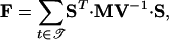16

where MV is the variance-covariance matrix of measurement errors and S is the sensitivity matrix: 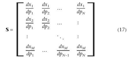for a model with M considered states and N parameters. Because the state variables are time-dependent, the sensitivities are also time-dependent. A set of M · N differential equations has to be solved together with the M model equations (Varma et al. 1999):

18

Having solved the equations, the Fisher-Information-Matrix is calculated according to equation 16 by summing up all values over the time span. The Fisher-Information-Matrix is the inverse of the parameter estimation error covariance matrix of the best linear unbiased estimator (Posten and Munack 1990). The standard deviations of the parameters are therefore the square roots of the diagonal elements of F^-1. They are, however, only lower bounds for the standard deviations, because the system is nonlinear in the parameters (Ljung 1999; Banga et al. 2002):

19

The corresponding 95% confidence intervals can be approximated by two times the standard deviation (Press et al. 2002):

20

and are displayed in Figure 3 by solid lines. The figure shows relative confidence intervals Δp_i, that is, the confidence intervals have been normalized by the estimated parameters, given in Table 3. Thus, a value of 1 corresponds to the estimated parameter being equal to the optimal parameter value. For K_I, the calculated 95% confidence interval includes negative values, because a normal distribution was assumed, which is obviously not correct in this case.

Figure 3.

Parameter confidence intervals and box-plot. The parameter confidence intervals are shown normalized to the optimal values attained for the benchmark measurements. The 95% confidence interval based on the Fisher-Information-Matrix is depicted by the solid lines. The box-plot depicts the results of the bootstrap method. For both models, the estimated 95% interval for K_I includes negative values. Therefore, the whole interval is not depicted here.

The second approach estimates the “true” spreading of the parameters by repeating the parameter fitting to a large number of experiments, a so-called bootstrapping approach (Press et al. 2002). Here, 50 repeats were performed using the given Web site. In practice, such a large number of experiments would rarely be possible. Instead, “new experiments” can be generated by randomly picking a certain number of data points and moving them according to the uncertainty model of the corresponding measurement. The bootstrap approach estimates not only a mean and standard deviation of the parameter distribution, but also its shape. This can be visualized using a box-plot as depicted in Figure 3. A box-plot is a graphical representation of an ordered set of numbers. It depicts the median value by the central line. The median is the center value of a sorted list of data and is preferred to the mean as it is less sensitive to outliers in the data. The box shows where the central 50% of the values are, the so-called second and third quantiles. The vertical bars indicate how the remaining values are distributed. To eliminate the influence of outliers, the length of these bars is usually bounded. Here, 1.5 times the height of the box is used as maximal extension. The box-plot in Figure 3, for example, shows that the distribution is not symmetric, but that values larger than the median are spreading more than those below the median.

Clearly, the results of the two approaches differ quite substantially. This is due to nonlinear behavior of the system. Although the first approach (calculating F) assumes that the system is linear with respect to the parameters, the bootstrap approach is not based on a linearization. Its drawback is that the underlying experiment needs to be repeated several times. As high-throughput experiments become more common, bootstrap approaches might become more feasible in the future.

As expected, the estimation of parameter Y_X/S yields almost identical values for both models (see Table 3). For the other parameters, the differences lie within the respective confidence intervals. Both models achieve a good agreement between the measurements and the simulated data, as observed from the attained objective functions in Table 3 and Figure 4. Discriminating between the two enzymatic hypotheses is therefore not possible.

Figure 4.

Benchmark data points (▵, ○) versus the simulated time courses of Model A (solid) and Model B (dashed) using the parameters of Table 3. Upper left: X solid, S dashed; upper right: M1; lower left: M2; lower right: M3.

Solutions for Model Discrimination

In the following sections, different approaches to the model discrimination problem are discussed, and every approach suggests a new design experiment. All solutions presented here are based on the same structure of the model equations, as given in “Model Formulation” above.

Large Steps on the Inputs

The idea was to look for simple profiles of the manipulated variables, which can easily be implemented in a real world experiment. One simple possibility investigated here is applying large changes on the two inputs q_in = q_out and c_in. This can result in an enhancement of small differences between the time curves calculated using the two tested models.

The strategy used in this section comprises (1) calculation of the steady state of four initial cases with low or high values of the feed concentration c_in and flow rates q_in = q_out; (2) simulation of 12 different step experiments (four different initial conditions each with three different input changes: rate, concentration, and both) for both models; (3) fitting of the model parameters for each experiment and both models. Thus, 24 parameter sets are obtained, and the respective objective functions are calculated; (4) comparison of the resulting objective functions of Models A and B for each experiment. The objective functions for one experiment are different for both models if one model describes well the obtained data (low objective function) and the other does not (large objective function). Based on this comparison, the most discriminating experiment can be chosen. If the experimental data for the 12 versions of the second experiment would not be available, the parameter fitting step (3) was eliminated and the differences between both simulated time curves (using Models A and B) of every model state were used to identify the most discriminating experiment (4). Therefore, the model parameters based on the benchmark experiment would be used.

The most discriminating step that is suggested as a new experiment is summarized in Table 4. Starting in steady-state conditions with high flow rate and high feed concentration after 24 h, a change in the concentration is performed resulting in high-flow-rate and low-feed-concentration conditions. Several similarly discriminating cases were found but were not used in the following. For the rest of the possibilities, either poor fits to the Web site data and/or lower differences in the objective function were obtained (data not shown).

Table 4.

Experimental Procedure for Model Discrimination

Time (h)	Cin (g/L)	qin, qout (L/h)
0-24	2.0	0.4
24-60	0.1	0.4

The new parameters for Model B are close to those attained by fitting only the benchmark experiment (see Table 5). The parameters of Model A, however, are quite different, in particular, K_I. The benchmark and the new experiment can be well fitted by Model B—see M3 in Figure 5. However, the Model A with the new parameter set is not any more able to fit M3 in the benchmark or the new experiment. Differences can be found all over the simulated time span, whereas the highest differences can be seen after the applied step (24 h) in the new experiment—see Figure 5. The time curves for biomass, substrate, and metabolites M1 and M2 show almost no differences between the two models. From the above, it can therefore be concluded that Model A can be discarded and that Model B describes the benchmark problem better with the proposed parameters. The control of the enzyme is realized by regulation of enzyme synthesis.

Table 5.

Identified Parameters of Both Models, Attained by Minimizing the Objective Function (15) Over the New and the Benchmark Experiment

Parameter	Model A	Model B
Yx/s	6.7 × 10−5 g/μmol	6.7 × 10−5 g/μmol
KIA	4.8 μmol/gDW	—
KIB	—	8.9 × 10−3 μmol/gDW
k2	2.3 × 106 L/h	3.2 × 106 L/h
ksynmax	8.2 × 10−3 μmol/gDW h	1.8 × 10−2 μmol/gDW h

Figure 5.

Data points of metabolite M3 (○) versus simulated time courses of Model A (solid) and Model B for the benchmark experiment (left) and the new experiment (right).

Linear Model Analysis—Analysis of the Phase Shift

The proposed solution is based on the linearized model. Regarding a steady-state solution (x^ss) during continuous fermentation (q_in = q_out = 0.25 L/h, c_in = 2.0 g/L), the linearized model is given by:

21

with the Jacobian

The input/output behavior of a linear system is characterized by two important observations: Stimulating the system with a given frequency w, the output shows the same frequency, but with a shift, named the phase shift, and amplified amplitude, named the gain. Linear dynamical model equations as given in equation 21 can be transformed to algebraic equations, called transfer functions, which can easily be handled.

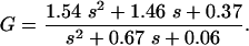
For the proposed method, the gain and the phase shift for the transfer functions G_ij = Y_i/U_j with outputs y₁ = M1, y₂ = M2, and y₃ = E are analyzed. For Models A and B, all parameters are fixed except parameters K_IA and K_IB, respectively. The values for K_IA and K_IB are varied in the range 5 × 10^-3 < K_I1/2 < 10.0. Figure 6 shows the phase shift for input q and output M1. As can be seen, there exists a small frequency span where the two models display different phase shifts for all parameter combinations. Therefore, an experiment should be performed that forces the system with a distinct frequency inside the frequency window to see whether Model A or Model B is correct. To verify the approach, a frequency of w = 0.5 1/h was chosen and phase shifts -6.2 < ΔΦ_A < -23.16, and -23.43 < ΔΦ_B < -31.18 for Models A and B, respectively, are expected. Figure 7 shows the time course of the input 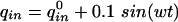and the time course of M1 (data from the Web site). With the given data it was not possible to fit parameters K_IA or K_IB with high quality. However, for the solution provided, only the phase shift must be determined. The data were fitted with a second-order transfer function G:

22

Figure 6.

Phase shift for input q on output c_M1. Solid lines show maximal and minimal values for Model A, whereas dashed lines show minimal and maximal values for Model B varying parameters K_IA and K_IB between 5 × 10^-3 and 10. For the small frequency span indicated by the vertical lines, the models are clearly separated (because of very small distances between the dashed lines, only one line can be seen).

Figure 7.

Time course of q_in (dashed), fitted (solid), and experimental values (circles) for M1; values are plotted minus mean values.

The phase shift for the given frequency w = 0.5 is ΔΦ = -28.38, indicating that Model B is correct. Note that the linear model with the correct parameters (but without noise) has a phase shift ΔΦ = -30.66 (see Appendix for the correct model).

Nonlinear Model Analysis

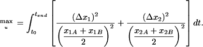
For the purpose of model discrimination, an experiment with an optimal input profile of the adjustable input variables (q_in, q_out, and c_in) has to be planned. For reasons of convenience, q_in and q_out are held equal here. The task can be formulated as the maximization of an objective function

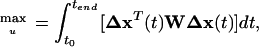23

with W being a weighting matrix and Δx being the difference between the responses of the two competing Models A and B (indexes A and B are used further to point to the model variants).

Many different approaches for the choice of the weighting matrix can be found in the literature. It is obvious that weighting should be done if the interesting state variables are within different orders of magnitude. In this case, it is useful to use a diagonal weighting matrix with elements:

24

that is, to weight by the average of the two models. The objective function for a simple example with two state variables (x₁ and x₂) reads:

25

It is, however, also possible to include information about the measurement variances, the variances of the parameters of the model, and the sensitivity of these parameters with respect to the interesting state variables. This can be useful, because the values of the parameters may be uncertain. Buzzi Ferraris et al. (1984) and Chen and Asprey (2003) introduced such a strategy. The weighting matrix is formulated as follows:

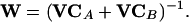
26

where VC is the variance-covariance matrix for model predictions:

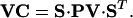27

PV is the parameter estimation error variance-covariance matrix (F^-1). It should be noticed that PV has to be approximated using the experiments carried out before, which in this case means only the benchmark experiment. Simplifying this approach by using only the diagonal elements of MV, PV, and VC clarifies its meaning: The squared model difference for one state variable is weighted by a sum given by its measurement variance, and the square of the sensitivity of each fitted parameter with respect to the state variable multiplied by the variance of the parameter. This means that the difference of a state variable contributes less to the objective function, if (1) the measurement error of that state variable is large and (2) the state variable in the designed experiment is very sensitive to parameters that could be estimated only with large errors using the experiment(s) carried out so far (here the benchmark experiment).

For a simple example with two state variables, the objective function looks now like this, if two parameters (index 1 and 2) are considered for each model:

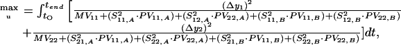28

Of course, this does not mean that VC has only diagonal elements (which would be mere chance), but that only the diagonal elements are considered in the approach.

This approach could help to avoid the case that an experiment is planned in which the model differences depend strongly on the value of parameters that are poorly fitted with the experiments carried out before. If the elements of MV are much larger than those of VC and the measurements have a similar standard variance (as in our case), it could be useful to use the following weighting matrix, that is, the simplified approach without consideration of the measurement variance:

29

More interesting parameters, namely, the influence of the considered model state variables, the definition of the weighting matrix, and the influence of the optimization method, are analyzed and discussed. In this particular case study, the model structure is such that the biomass and the concentration of the substrate do not depend on the choice of the model. Therefore, only metabolites M1, M2, and M3 are of interest. Measurements in biological systems are, however, often very time consuming. Therefore, it is important to identify the state variables that have to be measured for model discrimination.

Both using the stochastic method and using the gradient-based optimization method may have advantages. With the stochastic method, one cannot be caught in local optima, whereas the gradient method leads to more exact results. Therefore, both methods will be compared. Equations for the concentrations of the state variables of both models are used as described in the section on “Model Formulation” above. In the case of the gradient-based method, the objective function is maximized using dynamic optimization offered by the DIVA simulation environment (Ginkel et al. 2003). In the case of the stochastic method, the “Optimized Step-Size Random Search” (OSSRS) algorithm developed by Sheela (1979) is used.

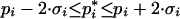
As a result of these considerations, optimization with several objective functions, differing in the weighting matrices used and the state variables or combinations of state variables considered, was performed with both optimization methods. For the calculations, the following conditions are fixed:

• Input moves are allowed every 10 h.

• The integration time is 60 h.

• The constraints used are given in Table 6. The biomass constraint ensures that washout is avoided. Moreover, there is enough biomass to be sampled out for the experimental measurements.

• The initial conditions for the state variables are chosen such that the steady-state values of both models are similar (stationary state with q = 0.25 L/h and c_in = 2.0 g/L).

• Parameter values for the models are as given in Table 3.

Table 6.

Constraints Used for Finding Optimal Input Profiles

Constraints	Value
Minimum flow rate	0.05 L/h
Maximum flow rate	1.60 L/h
Minimum feed concentration	0.50 g/L
Maximum feed concentration	10.0 g/L
Minimum volume	1.00 L
Maximum volume	5.00 L
Minimum biomass concentration	0.05 g/L

Table 7 summarizes the results obtained. A comparison between the values of the objective function can only be done for one approach, because it depends on the definition of W. The differences in the values of the objective function are very small between stochastic and gradient-based method for nearly all cases, although the obtained input profiles differ strongly (data not shown). This hints of the existence of several local optima with very similar values of the objective function. In some cases (e.g., case 21) the gradient-based method was, however, stuck to local optima of very low quality. For cases 1-14 (see Table 7), only state variable M1 contributes significantly to the objective function. Therefore, equally high values are reached for all cases in which M1 was included in the objective function and much lower values are obtained for the cases in which M1 was not included. For cases 15-28, only M2 contributes significantly to the objective function. Only the optimal cases (boldface in Table 7) for each approach have been followed up further.

Table 7.

Summary of Results of Nonlinear Model Analysis

			Optimization Method
Approach	Case	State Variables	Stochastic	Gradient-Based
No weighting	1	M1	3.7195 × 106	3.7342 × 106
	2	M2	9.0224 × 10−5	7.8716 × 10−5
	3	E	3.6658 × 10−4	8.015 × 10−7
	4	M1, M2	3.7198 × 106	3.7342 × 106
W, unity matrix	5	M1, E	3.7198 × 106	3.7342 × 106
	6	M2, E	3.6658 × 10−4	7.9476 × 10−5
	7	M1, M2, E	3.7195 × 106	3.7367 × 106
Weighted by square of average	8	M1	2.8287	2.8378
	9	M2	0.0222	0.1201
	10	E	0.0476	0.0493
W as in equation 24	11	M1, M2	2.8394	2.8428
	12	M1, E	2.8685	2.8806
	13	M2, E	0.0686	0.0692
	14	M1, M2, E	2.8739	2.8857
Simplified Chen and Asprey	15	M1	1.356	3.6054
	16	M2	36.3359	2.1768
	17	E	2.6896	0.099
	18	M1, M2	36.4986	7.6538
W as in equation 26	19	M1, E	2.6897	2.5091
	20	M2, E	36.9019	2.4782
	21	M1, M2, E	37.0645	7.763
Simplified Chen and Asprey without measurement variance	22	M1	24.88	22.9863
	23	M2	1.5598 × 1011	1.4355 × 1011
	24	E	3.6623	2.6398
	25	M1, M2	1.5598 × 1011	1.4355 × 1011
W as in equation 29	26	M1, E	24.88	3.6468
	27	M2, E	1.5598 × 1011	3.6207
	28	M1, M2, E	1.5598 × 1011	1.4355 × 1011

The following results are obtained from this first step: (1) the optimal input profiles differ strongly between the approaches and (2) none of the models can describe the experimental data with the set of parameters derived from the benchmark experiment. Figure 8 shows exemplarily in silico experimental and simulation data for case 23 (W as in equation 29, consideration of M2). Parameter fitting was therefore repeated in a second step with measurements from both experiments, the benchmark experiment and the new experiment, for the indicated cases.

Figure 8.

Optimal experiment, designed with W as in equation 29 (case 23). Optimal input profiles, in silico measurement results (circles), and results obtained with Model A (solid line) and Model B (dashed line) with the initial sets of parameters. Differences between the results of the two models are most notable in M1.

After parameter estimation, Model A can be excluded in all cases, because the simulation of the enzyme does not fit the benchmark experiment. Figure 9 (left) shows this result exemplarily for case 1 (without weighting, consideration of only M1). The corresponding parameters can be found in Table 8. Exclusion of Model A could be verified by an F-test. The F-test uses the ratio of the standard deviations of two data sets and tests the null hypothesis that they are not significantly different. The standard deviations S of the residuals for the enzyme were calculated to be 1.7133 × 10^-4 for Model A and 1.0104 × 10^-5 for Model B. The level of significance was chosen to be α = 0.99 and the data sets contained both 30 residuals.

Figure 9.

(Left) Enzyme concentration in benchmark experiment after fitting with the benchmark experiment and designed experiment for case 1. (Right) Enzyme concentration in the designed experiment (case 23) after fitting with the benchmark experiment and the designed experiment for case 23. In silico measurement results (circles) and results obtained with Model A (solid line) and Model B (dashed line). Results of Model A do not fit.

Table 8.

Identified Parameters of Both Models, Attained by Minimizing the Objective Function (15) Over the New Experiment Designed Without Weighting and the Benchmark Experiment

Parameter	Model A	Model B
KIA	0.0138 μmol/gDW	—
KIB	—	0.0136 μmol/gDW
k2	22.4 × 106 L/h	6.05 × 106 L/h
Ksynmax	0.00366 μmol/gDW h	0.0135 μmol/gDW h

This means that the null hypothesis has to be rejected and the residuals of Model B have a significantly lower standard deviation than those of Model A. For the other weighting matrices, similar results were obtained (data not shown).

The findings of the proposed approach are discussed in the following: first, the focus is on the question of which model state variables have to be measured. Interestingly, the enzyme did not contribute significantly to the objective functions of all the approaches studied. The conclusion could have been, that it is not necessary to measure the enzyme. In the simulation results of the designed experiments, there are big differences in M1 and M2 between the two models, but both models can describe M1 and M2 after fitting. Therefore, without measurements of the enzyme, none of the models would have been able to discriminate between the two models after fitting.

The second question focuses on the weighting matrix that leads to the best results. All of the approaches could discriminate between the two models. It could, however, be seen as an advantage of the last approach (equation 29) that the simulation for the enzyme with Model A does additionally not fit measurements for the designed experiment (case 23; Fig. 9, right). This could again be verified by an F-test with a level of significance α = 0.99. The standard deviations S of the residuals for the enzyme were calculated to be 0.0093 for Model A and 2.6202 × 10^-4 for Model B. There were 30 measurements within the designed experiment, and

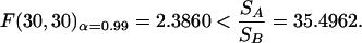Figure 10 shows parameter confidence intervals for the following exemplary cases: (a) using only the benchmark experiment for parameter fitting, (b) using only the experiment case 1 (without weighting, consideration of M1), (c) using only the experiment case 23 (W as in equation 29, consideration of M1 and M2), and (d) using both the benchmark experiment and the experiment case 1. Each designed experiment leads to a reduction of the parameter confidence intervals, especially for parameters K_IA and K_IB, respectively. Case a shows by far the lowest values, lower than those obtained by using the two experiments in case d.

Figure 10.

(Left) Parameter confidence intervals for Model A. (Right) Parameter confidence intervals for Model B. Four cases are compared. From left to right 1 (dot): experiment with W as in equation 29; 2 (solid) benchmark experiment; 3 (dashed) experiment obtained without weighting; 4 (dash-dot) benchmark experiment and experiment obtained without weighting.

Third, the influence of the optimization method was analyzed. Both the stochastic and the gradient-based methods lead to similar results. Using the stochastic method ensures, however, that one is not stuck in a significantly suboptimal local optimum. On the other hand, the stochastic method is very time consuming.

DISCUSSION

A benchmark problem for reverse engineering, parameter identification, and model discrimination is presented. The focus of the investigation at hand lies on model discrimination. It is shown that for a problem that may arise in microbiology or cell biology, the application of system-theoretical methods allows one to come to satisfactory results without constructing several mutant strains. However, the application of the methods requires that the cellular system can be stimulated from outside. If a bioreactor system is available, the feed rate and the feed concentration may be used. For all methods, dynamical measurements, that is, time courses of interesting variables, are essential. Based on new measurement technologies like cDNA-arrays or proteomics, it is expected that such measurements are available in the near future. Clearly, the methods are general and do not depend on the special biochemical circuit under consideration.

Three methods for experimental design have been presented that were all able to discriminate between two model variants. Several parameters, namely, the influence of model state variables and control inputs, the definition of weighting matrices, and the influence of the optimization method were analyzed. In the case at hand, the problem is formulated in such a way that biomass and concentration of the substrate do not depend on the choice of the model. Only intracellular metabolites, M1, M2, and M3, are of interest. Measurements in biological systems are, however, often very time consuming. Therefore, it is important to identify the state variables that have to be measured for model discrimination. Given in silico experimental data, two model variants are formulated, and it was shown that both models are able to describe the given data.

Application of the three methods led to very different input profiles for inputs q and c_in in the experiment designed for model discrimination. The first approach focuses on the largest possible steps on the system inputs by starting from values representing the limits of meaningful inputs. Simulation runs have been carried out for the resulting 12 experimental versions. The experiment that led to the largest differences between the objective functions (equation 15) of the models has been chosen to be the new experiment. This method represents a very intuitive approach.

The section on “Linear Model Analysis” above provides a more “sophisticated” solution based on the phase shift of the linearized models. Using this approach, the phase shift of the output has to be determined given a calculated input frequency. The only input/output combination that could be used here was the pair q, c_M1. Drawbacks of the approach are generating such an input (needs a process control system) and the length of the experiment, because only the tuned system can be analyzed. Because the approach is based on linear models, the input signal should be small to stay within the linear range of the model. This leads to very small changes in the desired output that can be difficult to measure in a real-world experiment.

The third approach discriminates the models by bringing the states as apart as possible, however weighting the differences of the state variables. A method recently proposed by Chen and Asprey (2003) was simplified to clarify the weights used. The method calculates an input profile in such a way that the difference of a state variable contributes less to the objective function if the measurement error of that state variable is large and if the state variable in the designed experiment is very sensitive to parameters that could hardly be estimated using the benchmark experiment. Nonlinear optimization leads to very different input profiles, depending on the weighting matrices used and on the optimization method. One of these profiles represents also a form of large steps in the inputs (see Fig. 8), but the resulting differences in enzyme concentration are larger than those obtained by the first approach (cf. Figs. 5 and 9).

Common to all the methods is the observation that performing the newly designed experiment (here, with the interactive Web site) results in rather bad model predictions, if the in silico data are compared with the simulation. This is based on the large variance of the parameters determined in the initial experiment. Therefore, the parameters had to be identified again and Model A was excluded as a candidate model, because one state variable could not be fitted with both experiments. Interestingly, this state variable (M3) did not significantly contribute to the objective functions.

The model used for the Web interface is given in the Appendix. It is composed of both control of the enzyme activity and control of enzyme synthesis. However, the influence of control of enzyme activity, represented by parameter K_IA, is very small. Therefore, the choice of Model B is the correct one. Comparing the parameters estimated in the first and third approaches and the correct parameters given in the Appendix (Table 9), the third approach gets better results. Moreover, the confidence region for the parameters is almost always smaller than for the benchmark experiment. For the second approach, the re-estimation of parameters is not necessary. However, one has to determine the phase shift for the frequency calculated that will last some time, because the system has to be tuned.

Table 9.

Additional Parameters of the Correct Model

Parameter	Value
Yx/s	7.0 × 10−5 g/μmol
KIA	0.01 μmol/gDW −
KIB	10.0 μmol/gDW
k2	6.0 × 106 L/h
ksynmax	0.0168 μmol/gDW h

Based on our results, it is not possible to recommend one of these approaches. The application of one of these methods depends strongly on the possibilities to stimulate the system and to obtain measurements with high quality. The first method could be performed as a first initial experiment if there was little time to optimize the system. Comparing the stochastic versus the gradient-based optimization methods, the former leads to better results. However, the computational effort for this method is very high, as the calculation may last some days.

Another concern of this paper was the explanation and comparison of two methods for the determination of parameter accuracy. A very common method for this purpose is the approximation of parameter variances by use of the Fisher-Information-Matrix. The parameter variances obtained by this method represent, however, only lower bounds, that is, the actual variances will be larger. Furthermore, calculating the 95% confidence intervals as two times the standard deviations, as was done in this contribution, implies a normal distribution of the parameters. It is, therefore, not surprising that application of the bootstrapping approach, which does not have these drawbacks, leads to very different results (although the proportions between the parameters are similar). They represent the “true” spreading of the parameters. For the application of this method, either the possibility of repeating the experiment several times or the existence and application of an uncertainty model of the corresponding measurement are necessary. As high-throughput experiments become more common, bootstrapping approaches might become more feasible in the future.

APPENDIX

Measurement

time [h]	X [g/l]	S [g/l]
0	0.1088	1.9134
2.0000	0.4345	0.0805
4.0000	0.4811	0.0791
6.0000	0.4114	0.0734
8.0000	0.3956	0.0990
10.0000	0.3714	0.0724
12.0000	0.3995	0.0782
14.0000	0.4477	0.0752
16.0000	0.4190	0.0853
18.0000	0.3540	0.0725
20.0000	0.3690	0.0781
22.0000	0.4345	0.1195
24.0000	0.3183	0.1178
26.0000	0.3767	0.1099
28.0000	0.3489	0.1243
30.0000	0.4019	0.1249
32.0000	0.2023	0.0403
34.0000	0.1595	0.0703
36.0000	0.1068	0.0691
38.0000	0.0868	0.0933
40.0000	0.1047	0.0893
42.0000	0.0967	0.1000
44.0000	0.0714	0.0965
46.0000	0.0916	0.1122
48.0000	0.0992	0.1234
50.0000	0.0877	0.1180
52.0000	0.0766	0.1133
54.0000	0.0747	0.1196
56.0000	0.0769	0.1256
58.0000	0.0786	0.1269
60.0000	0.0781	0.1138
M1	M2	M3
0.0620	0.0079	0.0749
0.4479	0.0110	0.0124
0.3045	0.0102	0.0173
0.2534	0.0133	0.0266
0.2569	0.0116	0.0294
0.2736	0.0125	0.0378
0.2561	0.0130	0.0257
0.2268	0.0112	0.0332
0.2086	0.0121	0.0305
0.2375	0.0121	0.0296
0.2539	0.0128	0.0342
0.4895	0.0169	0.0258
0.4561	0.0147	0.0176
0.4673	0.0173	0.0187
0.5358	0.0144	0.0152
0.5961	0.0149	0.0156
0.1357	0.0067	0.0319
0.1584	0.0089	0.0432
0.1873	0.0121	0.0418
0.2860	0.0138	0.0296
0.3434	0.0135	0.0322
0.4408	0.0152	0.0267
time [h]	X [g/l]	S [g/l]
0.4767	0.0161	0.0225
0.5163	0.0180	0.0222
0.5675	0.0165	0.0189
0.5399	0.0181	0.0202
0.5851	0.0177	0.0176
0.6062	0.0157	0.0157
0.5443	0.0128	0.0205
0.6399	0.0143	0.0154
0.6020	0.0127	0.0142

The values of M1, M2, and M3 are in [μmol/gDW]. A file with the presented data can be downloaded from the Web site.

The Correct Model

The correct model is given by:

30

31

32

For reaction rates r₁, r₂, and r₃ the following equations hold:

33

34

35

Enzyme synthesis is taken into account with:

36

The following system of equations for the concentrations of M1, M2, and E is obtained for both models:

37

38

39

To describe the growth rate, it is assumed that part of the substrate taken up by the organisms is converted into biomass with a yield coefficient Y_xs. The equation for μ is:

40

The correct parameters are summarized in Table 9.

References

- Arkin, A. and Ross, J. 1995. Statistical construction of chemical reaction mechanisms from measured time series. J. Phys. Chem. 99: 970-979. [Google Scholar]
- Arkin, A., Shen, P., and Ross, J. 1997. A test case of correlation metric construction of a reaction pathway from measurements. Science 277: 1275-1279. [Google Scholar]
- Asprey, S.P. and Macchietto, S. 2000. Statistical tools for optimal dynamic model building. Comput. Chem. Eng. 24: 1261-1267. [Google Scholar]
- Banga, J.R., Versyck, K.J., and Van Impe, J.F. 2002. Computation of optimal identification experiments for nonlinear dynamic process models: A stochastic global optimization approach. Ind. Eng. Chem. Res. 41: 2425-2430. [Google Scholar]
- Box, G.E.P. and Hill, W.J. 1967. Discrimination among mechanistic models. Technometrics 9: 57-71. [Google Scholar]
- Buzzi Ferraris, G., Forzatti, P., Emig, G., and Hofmann, H. 1984. Sequential experimental design for model discrimination in the case of multiple responses. Chem. Eng. Sci. 39: 81-85. [Google Scholar]
- Chen, H. and Asprey, S.P. 2003. On the design of optimally informative dynamic experiments for model discrimination in multiresponse nonlinear situations. Ind. Eng. Chem. Res. 42: 1379-1390. [Google Scholar]
- Cooney, M.J. and McDonald, K.A. 1995. Optimal dynamic experiments for bioreactor model discrimination. Appl. Microbiol. Biotechnol. 43: 826-837. [DOI] [PubMed] [Google Scholar]
- D'haesseleer, P., Liang, S., and Somogyi, R. 2000. Genetic network inference: from co-expression clustering to reverse engineering. Bioinformatics 16: 707-726. [DOI] [PubMed] [Google Scholar]
- Faller, D., Klingmüller, U., and Timmer, J. 2003. Simulation methods for optimal experimental design in systems biology. Simulation 79: 717-725. [Google Scholar]
- Ginkel, M., Kremling, A., Nutsch, T., Rehner, R., and Gilles, E.D. 2003. Modular modeling of cellular systems with ProMoT/Diva. Bioinformatics 19: 1169-1176. [DOI] [PubMed] [Google Scholar]
- Ideker, T., Thorsson, V., Ranish, J.A., Christmas, R., Buhler, J., Eng, J.K., Bumgarner, R., Goodlett, D.R., Aebersold, R., and Hood, L. 2001. Integrated genomic and proteomic analyses of a systematically perturbed metabolic network. Science 292: 929-934. [DOI] [PubMed] [Google Scholar]
- Kitano, H. 2000. Perspectives on systems biology. New Generation Computing 18: 199-216. [Google Scholar]
- Koza, J.R., Mydlowec, W., Lanza, G., Yu, J., and Keane, M.A. 2001. Reverse engineering of metabolic pathways from observed data using genetic programming. In Proceedings of the 6th Pacific Symposium on Biocomputing, Hawaii, USA (eds. R.B. Altmann and A.K. Dunker), pp. 434-445. World Scientific Publishing Company. [DOI] [PubMed]
- Kremling, A., Bettenbrock, K., Laube, B., Jahreis, K., Lengeler, J.W., and Gilles, E.D. 2001. The organization of metabolic reaction networks: III. Application for diauxic growth on glucose and lactose. Metab. Eng. 3: 362-379. [DOI] [PubMed] [Google Scholar]
- Ljung, L. 1999. System Identification—Theory for the user, 2nd ed. Prentice Hall PTR, Upper Saddle River, NJ.
- Moles, G., Mendes, P., and Banga, J.R. 2003. Parameter estimation in biochemical pathways: A comparison of global optimization methods. Genome Res. 13: 2467-2474. [DOI] [PMC free article] [PubMed] [Google Scholar]
- Munack, A. 1992. Some improvements in the identification of bioprocesses. In Modeling and control of biotechnical processes 1992, IFAC Symposia series (eds. M.N. Karim and G. Stephanopoulos), pp. 89-94. IFAC, Pergamon Press, New York.
- Posten, C. and Munack, A. 1990. On-line application of parameter estimation accuracy to biotechnical processes. In Proceedings of the American Control Conference, Vol. 3, pp. 2181-2186. [Google Scholar]
- Press, W.H., Flannery, B.P., Teukolsky, S.A., and Vetterling, W.T. 2002. Numerical recipes in C: The art of scientific computing. Cambridge University Press, Cambridge, UK.
- Repsilber, D., Liljenström, H., and Andersson, S.G.E. 2002. Reverse engineering of regulatory networks: Simulation studies on a genetic algorithm approach for ranking hypotheses. BioSystems 66: 31-41. [DOI] [PubMed] [Google Scholar]
- Sheela, B.V. 1979. Optimized step-size random search (OSSRS). Computer Methods Appl. Mech. Engineer. 19: 99-106. [Google Scholar]
- Stelling, J., Kremling, A., Ginkel, M., Bettenbrock, K., and Gilles, E.D. 2001. Towards a virtual biological laboratory. In Foundations of systems biology (ed. H. Kitano), Chap. 9, pp. 189-212. The MIT Press, Cambridge, MA.
- Swameye, I., Miller, T.G., Timmer, J., Sandra, O., and Klingmüller, U. 2003. Identification of nucleocytoplasmic cycling as a remote sensor in cellular signaling by databased modeling. Proc. Natl. Acad. Sci. 100: 1028-1033. [DOI] [PMC free article] [PubMed] [Google Scholar]
- Tegner, J., Yeung, M.K.S., Hasty, J., and Collins, J.J. 2003. Reverse engineering gene networks: Integrating genetic perturbations with dynamical modeling. Proc. Natl. Acad. Sci. 100: 5944-5949. [DOI] [PMC free article] [PubMed] [Google Scholar]
- Varma, A., Morbidelli, M., and Wu, H. 1999. Parametric sensitivity in chemical systems. Cambridge University Press, Cambridge, UK.
- Zak, D.E., Gonye, G.E., Schwaber, J.S., and Doyle, F.J. 2003. Importance of input perturbations and stochastic gene expression in the reverse engineering of genetic regulatory networks: Insights from an identifiability analysis of an in silico network. Genome Res. 13: 2396-2405. [DOI] [PMC free article] [PubMed] [Google Scholar]
WEB SITE REFERENCES
- http://www.sysbio.de/projects/benchmark/; Interactive Web site with online model.