Traveling wave solutions of the time-delayed generalized Burgers-type equations

Abstract

Background

Recently, nonlinear time-delayed evolution equations have received considerable interest due to their numerous applications in the areas of physics, biology, chemistry and so on.

Methods

In this paper, we obtain traveling wave solutions by using the extended $\left(\frac{G^{\prime }}{G}\right)$-expansion method.

Results

Based on the method, we get many solutions of the time-delayed generalized Burgers-type equations.

Conclusions

The results reveal that the extended $\left(\frac{G^{\prime }}{G}\right)$-expansion method is direct, effective and can be used for many other nonlinear time-delayed evolution equations.

Background

In recent years, theory and numerical analysis of nonlinear time-delayed evolution equations have received considerable interest due to their numerous applications in the areas of physics, biology, chemistry and so on. For better studying the nonlinear physical phenomena of nonlinear time-delayed evolution equations, the solution is much involved. In the past, several analytical and numerical methods have been used to find solutions of nonlinear partial differential equations, such as homotopy perturbation method (Kumar and Singh 2009; Kumar et al. 2012; He 1999), Laplace transform (Kumar 2014), variational iteration method (He 1997; He and Wu 2007; Tang et al. 2014), residual power series method (RPSM for short) (Kumar et al. 2016b; Yao et al. 2015), auxiliary equation method (Sirendaoreji 2003; Tang et al. 2016; Yomba 2004), homotopy analysis method (Yin et al. 2015; Kumar et al. 2016a), $\left(\frac{G^{\prime }}{G}\right)$-expansion method (Wang et al. 2008; Zhang et al. 2010; Tang et al. 2011; Islam et al. 2014; Khan and Akbar 2014) and so on.

In this paper, we apply the extended $\left(\frac{G^{\prime }}{G}\right)$-expansion method to obtain traveling wave solutions of the following time-delayed generalized Burgers-type equations (Kar et al. 2003):

• The time-delayed generalized Burgers equation:

  $$\mathit{\tau }{v}_{tt}+v_t+p{v}^s{v}_x-v_{xx}=0.$$

  where p, s are constants and $\mathit{\tau }$is a time-delayed constant.
• The time-delayed generalized Burgers-Fisher equation:

  $$\mathit{\tau }{v}_{tt}+(1-\mathit{\tau }{f}_v)v_t=v_{xx}-p{v}^s{v}_x+f(v),f(v)=qv(1-v^s).$$

This paper is organized as follows: in “Methods” section, the main steps of extended $\left(\frac{G^{\prime }}{G}\right)$-expansion method for obtaining traveling wave solutions of nonlinear time-delayed evolution equation are given. In “Results” section, we construct traveling solutions of the time-delayed generalized Burgers-type equation. Some conclusions are given in “Conclusions” section.

Methods

Considering the following nonlinear evolution equation:

$$P(v,v_t,v_{x_1},v_{x_2},v_{x_3},\dots )=0,$$ 1

where P is a polynomial in $v=v(x_1,x_2,x_3,\dots ,t)$ and its various partial derivatives.

Step 1

By means of the traveling wave transformation

$$v=V(\mathit{\eta }),\mathit{\eta }=k_1{x}_1+k_2{x}_2+k_3{x}_3+\cdots +ht+{\mathit{\eta }}_0,$$ 2

where the coefficients $k_i$, h are constants. Equation (1) can be transformated as follows:

$$P(V(\mathit{\eta }),V^{\prime }(\mathit{\eta }),V^{{}^{″}}(\mathit{\eta }),\dots )=0.$$ 3

Step 2

We suppose that the Eq. (3) has the following solution:

$$V(\mathit{\eta })=\sum _{l=-n}^n{a}_l{\left(\frac{G^{\prime }}{G}\right)}^l,$$ 4

where $a_l$ are constants to be determined later, and $G(\mathit{\eta })$ satisfies the following equation:

$$G^{″}(\mathit{\eta })+\mathit{\alpha }{G}^{\prime }(\mathit{\eta })+\mathit{\beta }G(\mathit{\eta })=0,$$ 5

where $\mathit{\alpha }$ and $\mathit{\beta }$ are arbitrary constants. Based on Eq. (5), we have

$$\frac{G^{\prime }(\mathit{\eta })}{G(\mathit{\eta })}=\left\{\begin{array}{cc}-\frac{\mathit{\alpha }}{2}+\frac{\sqrt{{\mathit{\alpha }}^2-4\mathit{\beta }}}{2}\left(\frac{C_{1}sinh\left(\frac{\sqrt{{\mathit{\alpha }}^2-4\mathit{\beta }}\mathit{\eta }}{2}\right)+C_{2}cosh\left(\frac{\sqrt{{\mathit{\alpha }}^2-4\mathit{\beta }}\mathit{\eta }}{2}\right)}{C_{1}cosh\left(\frac{\sqrt{{\mathit{\alpha }}^2-4\mathit{\beta }}\mathit{\eta }}{2}\right)+C_{2}sinh\left(\frac{\sqrt{{\mathit{\alpha }}^2-4\mathit{\beta }}\mathit{\eta }}{2}\right)}\right),\hfill & {\mathit{\alpha }}^2-4\mathit{\beta }>0,\hfill \\ -\frac{\mathit{\alpha }}{2}+\frac{\sqrt{4\mathit{\beta }-{\mathit{\alpha }}^2}}{2}\left(\frac{-C_{1}sin\left(\frac{\sqrt{4\mathit{\beta }-{\mathit{\alpha }}^2}\mathit{\eta }}{2}\right)+C_{2}cos\left(\frac{\sqrt{4\mathit{\beta }-{\mathit{\alpha }}^2}\mathit{\eta }}{2}\right)}{C_{1}cos\left(\frac{\sqrt{4\mathit{\beta }-{\mathit{\alpha }}^2}\mathit{\eta }}{2}\right)+C_{2}sin\left(\frac{\sqrt{4\mathit{\beta }-{\mathit{\alpha }}^2}\mathit{\eta }}{2}\right)}\right),\hfill & {\mathit{\alpha }}^2-4\mathit{\beta }<0.\hfill \\ \frac{C_2}{C_1+C_2\mathit{\eta }}-\frac{\mathit{\alpha }}{2},\hfill & {\mathit{\alpha }}^2-4\mathit{\beta }=0.\hfill \end{array}\right.$$

Step 3

Determine the degree n in Eq. (3) by use of homogenous balanced principle (Abdel Rady et al. 2010; Fan and Zhang 1998a, b; Senthilvelan 2001; Zhao and Tang 2002; Fan 2000; Eslami et al. 2014), namely balancing the highest order derivatives and nonlinear terms in Eq. (3).

Step 4

Substituting Eqs. (4) and (5) into Eq. (3) and clearing the denominator and collecting all terms with the same order of $\left(\frac{G^{\prime }}{G}\right)$ together, then setting each coefficient of ${\left(\frac{G^{\prime }}{G}\right)}^l$ to zero, we get a system of under-determined algebraic equations for $k_i,h$ and $a_l$.

Step 5

Solving the algebraic equations in Step 4 by Maple (www.maplesoft.com), we can finally get traveling wave solutions of Eq. (1).

Results

In this section, we apply the extended $\left(\frac{G^{\prime }}{G}\right)$-expansion method to obtain traveling wave solutions of the time-delayed generalized Burgers-type equations.

Solutions to the time-delayed generalized Burgers equation

We consider the following time-delayed generalized Burgers equation:

$$\mathit{\tau }{v}_{tt}+v_t+p{v}^s{v}_x-v_{xx}=0.$$ 6

By using transformations $v(x,t)=V(\mathit{\eta })$ and $\mathit{\eta }=k(x-\mathit{\omega }t)$, Eq. (6) can be reduced as follows:

$$(\mathit{\tau }{\mathit{\omega }}^2-1)k^2{V}^{″}-k\mathit{\omega }{V}^{\prime }+pk{V}^s{V}^{\prime }=0.$$ 7

Balancing $V^{″}$ with $V^s{V}^{\prime }$ gives $n=\frac{1}{s}$ which is not an integer as $s\ne 1$. So we use a transformation $V=W^{\frac{1}{s}}$ to change Eq. (7) into the form:

$$(\mathit{\tau }{\mathit{\omega }}^2-1)k^2\left[W^{″}W+\left(\frac{1}{s}-1\right)W^{\prime 2}\right]-k\mathit{\omega }{W}^{\prime }W+pk{W}^{\prime }{W}^2=0.$$ 8

We suppose that the solutions of (8) have the form (4) and (5), so

$$\begin{array}{cc}\hfill W^{\prime }(\mathit{\eta })=& \sum _{l=-n}^n{a}_l{\left(\frac{G^{\prime }}{G}\right)}^{l-1}\frac{G^{″}G-G^{\prime 2}}{G^2}\hfill \\ \hfill =& -\sum _{l=-n}^n{a}_l{\left(\frac{G^{\prime }}{G}\right)}^{l-1}\left[\mathit{\beta }+\mathit{\alpha }\left(\frac{G^{\prime }}{G}\right)+{\left(\frac{G^{\prime }}{G}\right)}^2\right],\hfill \\ \hfill W^{″}(\mathit{\eta })=& \sum _{l=-n}^n{a}_l{\left(\frac{G^{\prime }}{G}\right)}^{l-2}{\left[\mathit{\beta }+\mathit{\alpha }\left(\frac{G^{\prime }}{G}\right)+{\left(\frac{G^{\prime }}{G}\right)}^2\right]}^2\hfill \\ \hfill & +\sum _{l=-n}^n{a}_l{\left(\frac{G^{\prime }}{G}\right)}^{l-1}\left[\mathit{\alpha }+2\left(\frac{G^{\prime }}{G}\right)\right]\left[\mathit{\beta }+\mathit{\alpha }\left(\frac{G^{\prime }}{G}\right)+{\left(\frac{G^{\prime }}{G}\right)}^2\right].\hfill \end{array}$$

From above two equations, we can get the degrees of $W^{″}W$ and $W^{\prime }{W}^2$ are $2n+2$ and $3n+1$ respectively. Balancing $W^{″}W$ and $W^{\prime }{W}^2$ in Eq. (8) yields $2n+2=3n+1$, namely $n=1$. Therefore Eq. (8) have the following solutions:

$$W(\mathit{\eta })=\sum _{l=-1}^1{a}_l{\left(\frac{G^{\prime }}{G}\right)}^l.$$ 9

Substituting Eqs. (9) and (5) into Eq. (8), we get a set of under-determined algebraic equations for $a_l(l=0,\pm 1)$, $k,\mathit{\omega },\mathit{\alpha }$ and $\mathit{\beta }$.

$$\begin{array}{cc}\hfill {\left(\frac{G^{\prime }}{G}\right)}^4:& 2(\mathit{\tau }{\mathit{\omega }}^2-1)k{a}_1^2+\frac{k(\mathit{\tau }{\mathit{\omega }}^2-1)(1-s)a_1^2}{s}-p{a}_1^3=0,\hfill \\ \hfill {\left(\frac{G^{\prime }}{G}\right)}^3:& 3(\mathit{\tau }{\mathit{\omega }}^2-1)k\mathit{\alpha }{a}_1^2+2(\mathit{\tau }{\mathit{\omega }}^2-1)k{a}_1{a}_0\hfill \\ \hfill & +\frac{2k\mathit{\alpha }(\mathit{\tau }{\mathit{\omega }}^2-1)(1-s)a_1^2}{s}+\mathit{\omega }{a}_1^2-2p{a}_0{a}_1^2-p\mathit{\alpha }{a}_1^3=0,\hfill \\ \hfill {\left(\frac{G^{\prime }}{G}\right)}^2:& \frac{(\mathit{\tau }{\mathit{\omega }}^2-1)k(1-s)(-2a_1{a}_{-1}+2a_1^2\mathit{\beta }+a_1^2{\mathit{\alpha }}^2)}{s}+p{a}_0^2{a}_1(1+2\mathit{\alpha })\hfill \\ \hfill & +(\mathit{\tau }{\mathit{\omega }}^2-1)k({\mathit{\alpha }}^2+2\mathit{\beta })a_1^2+3(\mathit{\tau }{\mathit{\omega }}^2-1)k\mathit{\alpha }{a}_1{a}_0-p{a}_1^3\mathit{\beta }\hfill \\ \hfill & +2(\mathit{\tau }{\mathit{\omega }}^2-1)k{a}_1{a}_{-1}+\mathit{\omega }{a}_0{a}_1+\mathit{\omega }{a}_1^2\mathit{\alpha }-p{a}_1^2{a}_{-1}=0,\hfill \\ \hfill {\left(\frac{G^{\prime }}{G}\right)}^1:& \frac{(\mathit{\tau }{\mathit{\omega }}^2-1)k(1-s)(-4a_{-1}+2a_1\mathit{\beta })a_1\mathit{\alpha }}{s}-p{a}_1\mathit{\alpha }(a_1{a}_{-1}+a_0^2)\hfill \\ \hfill & +(\mathit{\tau }{\mathit{\omega }}^2-1)k{a}_1(a_1\mathit{\alpha }\mathit{\beta }+4a_{-1}\mathit{\alpha }+a_0{\mathit{\alpha }}^2+2a_0\mathit{\beta })\hfill \\ \hfill & -2p{a}_0{a}_1^2\mathit{\beta }+\mathit{\omega }{a}_1(a_0\mathit{\alpha }+a_1\mathit{\beta })=0,\hfill \\ \hfill {\left(\frac{G^{\prime }}{G}\right)}^0:& (\mathit{\tau }{\mathit{\omega }}^2-1)k(4a_{-1}{a}_1\mathit{\beta }+2a_{-1}{a}_1{\mathit{\alpha }}^2+a_0{a}_1\mathit{\beta }\mathit{\alpha }+a_{-1}{a}_0\mathit{\alpha })\hfill \\ \hfill & +(a_{-1}-a_1\mathit{\beta })(a_{-1}{a}_1+a_0^2)p-\mathit{\omega }{a}_0{a}_{-1}-\mathit{\omega }{a}_0{a}_1\mathit{\beta }\hfill \\ \hfill & +\frac{(\mathit{\tau }{\mathit{\omega }}^2-1)k(1-s)}{s}(-4a_{-1}{a}_1\mathit{\beta }-2a_{-1}{a}_1{\mathit{\alpha }}^2+a_{-1}^2+a_1^2{\mathit{\beta }}^2)=0,\hfill \\ \hfill {\left(\frac{G^{\prime }}{G}\right)}^{-1}:& (\mathit{\tau }{\mathit{\omega }}^2-1)k(4a_{-1}{a}_1\mathit{\alpha }\mathit{\beta }+2a_{-1}{a}_0\mathit{\beta }+a_{-1}{a}_0{\mathit{\alpha }}^2+a_{-1}^2\mathit{\alpha })\hfill \\ \hfill & -\mathit{\omega }{a}_{-1}(a_{-1}+a_0\mathit{\alpha })+p{a}_{-1}^2{a}_1\mathit{\alpha }+p{a}_{-1}{a}_0(2a_{-1}+a_0\mathit{\alpha })\hfill \\ \hfill & +\frac{(\mathit{\tau }{\mathit{\omega }}^2-1)k\mathit{\alpha }(1-s)}{s}(-4a_{-1}{a}_1\mathit{\beta }+2a_{-1}^2)=0,\hfill \\ \hfill {\left(\frac{G^{\prime }}{G}\right)}^{-2}:& \frac{(\mathit{\tau }{\mathit{\omega }}^2-1)k{a}_{-1}(1-s)}{s}(2a_{-1}\mathit{\beta }-2a_1{\mathit{\beta }}^2+a_{-1}{\mathit{\alpha }}^2)\hfill \\ \hfill & -\mathit{\omega }{a}_{-1}(a_{-1}\mathit{\alpha }+a_0\mathit{\beta })+p{a}_{-1}^2(2a_0\mathit{\alpha }+a_1\mathit{\beta })+p{a}_{-1}^3+p{a}_0^2{a}_{-1}\mathit{\beta }\hfill \\ \hfill & +(\mathit{\tau }{\mathit{\omega }}^2-1)k(2a_{-1}{a}_1{\mathit{\beta }}^2+3a_{-1}{a}_0\mathit{\alpha }\mathit{\beta }+2a_{-1}^2\mathit{\mu }+a_{-1}^2{\mathit{\alpha }}^2)=0,\hfill \\ \hfill {\left(\frac{G^{\prime }}{G}\right)}^{-3}:& \frac{2(\mathit{\tau }{\mathit{\omega }}^2-1)k{a}_{-1}^2\mathit{\alpha }\mathit{\beta }(1-s)}{s}+(\mathit{\tau }{\mathit{\omega }}^2-1)k{a}_{-1}\mathit{\beta }(2a_0\mathit{\beta }+3a_{-1}\mathit{\alpha })\hfill \\ \hfill & -\mathit{\omega }{a}_{-1}^2\mathit{\beta }+p{a}_{-1}^2(a_{-1}\mathit{\alpha }+2a_0\mathit{\beta })=0,\hfill \\ \hfill {\left(\frac{G^{\prime }}{G}\right)}^{-4}:& \frac{(\mathit{\tau }{\mathit{\omega }}^2-1)k{a}_{-1}^2{\mathit{\beta }}^2(1-s)}{s}+2(\mathit{\tau }{\mathit{\omega }}^2-1)k{a}_{-1}^2{\mathit{\beta }}^2+p{a}_{-1}^3\mathit{\beta }=0.\hfill \end{array}$$

Solving this algebraic equations by Maple, we can obtain the two results:

Case 1

$$\begin{array}{cc}& a_{-1}=\pm \frac{(s+1)\mathit{\beta }\mathit{\omega }}{p\sqrt{{\mathit{\alpha }}^2-4\mathit{\beta }}},a_0=\pm \frac{\mathit{\alpha }(s+1)\mathit{\omega }}{2p\sqrt{{\mathit{\alpha }}^2-4\mathit{\beta }}}+\frac{(s+1)\mathit{\omega }}{2p},\hfill \\ \hfill & a_1=0,k=\mp \frac{s\mathit{\omega }}{(\mathit{\tau }{\mathit{\omega }}^2-1)\sqrt{{\mathit{\alpha }}^2-4\mathit{\beta }}},\hfill \end{array}$$ 10

where $\mathit{\alpha }$, $\mathit{\beta }$ and $\mathit{\omega }$ are arbitrary constants.

Case 2

$$\begin{array}{cc}& a_{-1}=0,a_0=\pm \frac{\mathit{\alpha }(s+1)\mathit{\omega }}{2p\sqrt{{\mathit{\alpha }}^2-4\mathit{\beta }}}+\frac{(s+1)\mathit{\omega }}{2p},\hfill \\ \hfill & a_1=\pm \frac{(s+1)\mathit{\omega }}{p\sqrt{{\mathit{\alpha }}^2-4\mathit{\beta }}},k=\pm \frac{s\mathit{\omega }}{(\mathit{\tau }{\mathit{\omega }}^2-1)\sqrt{{\mathit{\alpha }}^2-4\mathit{\beta }}},\hfill \end{array}$$ 11

where $\mathit{\alpha }$, $\mathit{\beta }$ and $\mathit{\omega }$ are arbitrary constants.

Using Eqs. (9) and (10), we obtain the following solution of Eq. (6):

$$v_1(\mathit{\eta })={\left[\pm \frac{\mathit{\alpha }(s+1)\mathit{\omega }}{2p\sqrt{{\mathit{\alpha }}^2-4\mathit{\beta }}}+\frac{(s+1)\mathit{\omega }}{2p}\pm \frac{(s+1)\mathit{\beta }\mathit{\omega }}{p\sqrt{{\mathit{\alpha }}^2-4\mathit{\beta }}}{\left(\frac{G^{\prime }}{G}\right)}^{-1}\right]}^{\frac{1}{s}},$$ 12

where $\mathit{\eta }=\mp \frac{s\mathit{\omega }}{(\mathit{\tau }{\mathit{\omega }}^2-1)\sqrt{{\mathit{\alpha }}^2-4\mathit{\beta }}}(x-\mathit{\omega }t)$.

Based on Eqs. (9) and (11), we get the solution of Eq. (6) as follows:

$$v_2(\mathit{\eta })={\left[\pm \frac{\mathit{\alpha }(s+1)\mathit{\omega }}{2p\sqrt{{\mathit{\alpha }}^2-4\mathit{\beta }}}+\frac{(s+1)\mathit{\omega }}{2p}\pm \frac{(s+1)\mathit{\omega }}{p\sqrt{{\mathit{\alpha }}^2-4\mathit{\beta }}}\left(\frac{G^{\prime }}{G}\right)\right]}^{\frac{1}{s}},$$ 13

where $\mathit{\eta }=\pm \frac{s\mathit{\omega }}{(\mathit{\tau }{\mathit{\omega }}^2-1)\sqrt{{\mathit{\alpha }}^2-4\mathit{\beta }}}(x-\mathit{\omega }t)$.

Substituting the general solutions of Eq. (5) into Eq. (12), we have two kinds of travelling wave solutions as follows:

When ${\mathit{\alpha }}^2-4\mathit{\beta }>0$,

$$v(x,t)={\left[\frac{(s+1)\mathit{\omega }}{p\sqrt{{\mathit{\alpha }}^2-4\mathit{\beta }}}\left(\frac{\sqrt{{\mathit{\alpha }}^2-4\mathit{\beta }}\pm \mathit{\alpha }}{2}\pm \frac{2\mathit{\beta }}{-\mathit{\alpha }+\sqrt{{\mathit{\alpha }}^2-4\mathit{\beta }}\left(\frac{C_{1}sinh\frac{\sqrt{{\mathit{\alpha }}^2-4\mathit{\beta }}\mathit{\eta }}{2}+C_{2}cosh\frac{\sqrt{{\mathit{\alpha }}^2-4\mathit{\beta }}\mathit{\eta }}{2}}{C_{1}cosh\frac{\sqrt{{\mathit{\alpha }}^2-4\mathit{\beta }}\mathit{\eta }}{2}+C_{2}sinh\frac{\sqrt{{\mathit{\alpha }}^2-4\mathit{\beta }}\mathit{\eta }}{2}}\right)}\right)\right]}^{\frac{1}{s}},$$ 14

where $\mathit{\eta }=\mp \frac{s\mathit{\omega }}{(\mathit{\tau }{\mathit{\omega }}^2-1)\sqrt{{\mathit{\alpha }}^2-4\mathit{\beta }}}(x-\mathit{\omega }t)$.

When ${\mathit{\alpha }}^2-4\mathit{\beta }<0$,

$$v(x,t)={\left[\frac{(s+1)\mathit{\omega }}{p\sqrt{{\mathit{\alpha }}^2-4\mathit{\beta }}}\left(\frac{\sqrt{{\mathit{\alpha }}^2-4\mathit{\beta }}\pm \mathit{\alpha }}{2}\pm \frac{2\mathit{\beta }}{-\mathit{\alpha }+\sqrt{4\mathit{\beta }-{\mathit{\alpha }}^2}\left(\frac{-C_{1}sin\frac{\sqrt{4\mathit{\beta }-{\mathit{\alpha }}^2}\mathit{\eta }}{2}+C_{2}cos\frac{\sqrt{4\mathit{\beta }-{\mathit{\alpha }}^2}\mathit{\eta }}{2}}{C_{1}cos\frac{\sqrt{4\mathit{\beta }-{\mathit{\alpha }}^2}\mathit{\eta }}{2}+C_{2}sin\frac{\sqrt{4\mathit{\beta }-{\mathit{\alpha }}^2}\mathit{\eta }}{2}}\right)}\right)\right]}^{\frac{1}{s}},$$ 15

where $\mathit{\eta }=\mp \frac{s\mathit{\omega }}{(\mathit{\tau }{\mathit{\omega }}^2-1)\sqrt{{\mathit{\alpha }}^2-4\mathit{\beta }}}(x-\mathit{\omega }t)$.

Substituting the general solutions of Eq. (5) into Eq. (13), we have the following two kinds of travelling wave solutions:

When ${\mathit{\alpha }}^2-4\mathit{\beta }>0$,

$$u(x,t)={\left[\frac{(s+1)\mathit{\omega }}{2p}\pm \frac{(s+1)\mathit{\omega }}{2p}\left(\frac{C_{1}sinh\frac{\sqrt{{\mathit{\alpha }}^2-4\mathit{\beta }}\mathit{\eta }}{2}+C_{2}cosh\frac{\sqrt{{\mathit{\alpha }}^2-4\mathit{\beta }}\mathit{\eta }}{2}}{C_{1}cosh\frac{\sqrt{{\mathit{\alpha }}^2-4\mathit{\beta }}\mathit{\eta }}{2}+C_{2}sinh\frac{\sqrt{{\mathit{\alpha }}^2-4\mathit{\beta }}\mathit{\eta }}{2}}\right)\right]}^{\frac{1}{s}}$$ 16

where $\mathit{\eta }=\pm \frac{s\mathit{\omega }}{(\mathit{\tau }{\mathit{\omega }}^2-1)\sqrt{{\mathit{\alpha }}^2-4\mathit{\beta }}}(x-\mathit{\omega }t)$.

When ${\mathit{\alpha }}^2-4\mathit{\beta }<0$,

$$u(x,t)={\left[\frac{(s+1)\mathit{\omega }}{2p}\mp \frac{(s+1)\mathit{\omega }}{2p}i\left(\frac{-C_{1}sin\frac{\sqrt{4\mathit{\beta }-{\mathit{\alpha }}^2}\mathit{\eta }}{2}+C_{2}cos\frac{\sqrt{4\mathit{\beta }-{\mathit{\alpha }}^2}\mathit{\eta }}{2}}{C_{1}cos\frac{\sqrt{4\mathit{\beta }-{\mathit{\alpha }}^2}\mathit{\eta }}{2}+C_{2}sin\frac{\sqrt{4\mathit{\beta }-{\mathit{\alpha }}^2}\mathit{\eta }}{2}}\right)\right]}^{\frac{1}{s}}$$ 17

where $\mathit{\eta }=\pm \frac{s\mathit{\omega }}{(\mathit{\tau }{\mathit{\omega }}^2-1)\sqrt{{\mathit{\alpha }}^2-4\mathit{\beta }}}(x-\mathit{\omega }t)$.

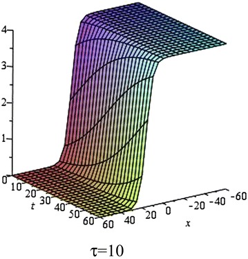
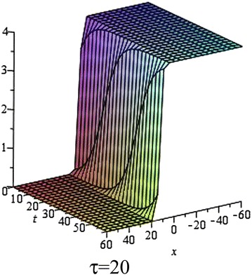
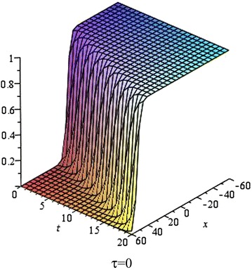
In Figs. 1, 2, 3 and 4, we show the effect of the time-delayed solution (14). It should be noted that when $\mathit{\tau }\to 0$, we can recover some traveling wave solutions of the generalized Burgers equation.

Fig. 1.

The solution (14) for $\mathit{\tau }=0$ at $s=1$, $p=0.1$, $\mathit{\omega }=0.2$, $\mathit{\alpha }=5$, $\mathit{\beta }=4$, $t=1$, $C_2=0$

Fig. 2.

The solution (14) for $\mathit{\tau }=10$ at $s=1$, $p=0.1$, $\mathit{\omega }=0.2$, $\mathit{\alpha }=5$, $\mathit{\beta }=4$, $t=1$, $C_2=0$

Fig. 3.

The solution (14) for $\mathit{\tau }=20$ at $s=1$, $p=0.1$, $\mathit{\omega }=0.2$, $\mathit{\alpha }=5$, $\mathit{\beta }=4$, $t=1$, $C_2=0$

Fig. 4.

The red, green and black lines represent the solution (14) for $\mathit{\tau }=0,10,20$ respectively at $s=1$, $p=0.1$, $\mathit{\omega }=0.2$, $\mathit{\alpha }=5$, $\mathit{\beta }=4$, $t=1$, $C_2=0$

Solutions to the time-delayed generalized Burgers–Fisher equation

In this section, we consider the time-delayed generalized Burgers–Fisher equation:

$$\mathit{\tau }{v}_{tt}+(1-\mathit{\tau }{f}_v)v_t=v_{xx}-p{v}^s{v}_x+f(v),f(v)=qv(1-v^s),q\ne 0.$$ 18

By using the transformation

$$v(x,t)=v(\mathit{\eta }),\mathit{\eta }=k(x-\mathit{\omega }t)$$ 19

Equation (18) is converted into the following ordinary differential equation:

$$k^2(\mathit{\tau }{\mathit{\omega }}^2-1)v^{″}-k\mathit{\omega }(1-\mathit{\tau }q+(s+1)q{v}^s)v^{\prime }+pk{v}^s{v}^{\prime }-qv(1-v^s)=0.$$ 20

Balancing $v^{″}$ and $v^s{v}^{\prime }$ in Eq. (20) gives $n=\frac{1}{s}$. By using the transformation $v=W^{\frac{1}{s}}$, we convert Eq. (20) into

$$\begin{array}{cc}& k^2(\mathit{\tau }{\mathit{\omega }}^2-1)\left(\frac{1}{s}-1\right)(W^{\prime 2}+W{W}^{″})-k\mathit{\omega }(1-\mathit{\tau }q+(s+1)qW)W{W}^{\prime }\hfill \\ \hfill & +pk{v}^2{W}^{\prime }-sq{W}^2(1-W)=0.\hfill \end{array}$$ 21

By balancing $W^{\prime 2}$ and $W^2{W}^{\prime }$ in Eq. (21), we suppose that Eq. (21) have the following solutions:

$$W(\mathit{\eta })=\sum _{l=-1}^1{a}_l{\left(\frac{G^{\prime }}{G}\right)}^l.$$ 22

Using the same procedure as in the previous example, we get a set of simultaneous algebraic equations for $a_l$, $k,\mathit{\omega },\mathit{\alpha }$ and $\mathit{\beta }$.

$$\begin{array}{cc}\hfill {\left(\frac{G^{\prime }}{G}\right)}^4:& -pk{a}_1^3+k\mathit{\omega }(s+1)q\mathit{\tau }{a}_1^3+(\mathit{\tau }{\mathit{\omega }}^2-1)k^2{a}_1^2\left(1+\frac{1}{s}\right)=0,\hfill \\ \hfill {\left(\frac{G^{\prime }}{G}\right)}^3:& k^2(\mathit{\tau }{\mathit{\omega }}^2-1)\left[2\left(1-\frac{1}{s}\right)\mathit{\alpha }{a}_1+a_0\right]a_1+k\mathit{\omega }(1-q\mathit{\tau })a_1^2\hfill \\ \hfill & +(\mathit{\omega }(s+1)-p)k(2a_0+\mathit{\alpha }{a}_1)a_1^2+sq{a}_1^3=0,\hfill \\ \hfill {\left(\frac{G^{\prime }}{G}\right)}^2:& \frac{k^2(\mathit{\tau }{\mathit{\omega }}^2-1)a_1}{s}(({\mathit{\alpha }}^2+2\mathit{\beta })a_1+(2s-1)a_{-1}+3a_0\mathit{\alpha }s)\hfill \\ \hfill & -pk{a}_1(a_{-1}{a}_1+a_0+2\mathit{\alpha }{a}_0{a}_1+a_1^2\mathit{\beta })+k\mathit{\omega }(1-q\mathit{\tau })(a_0+a_1\mathit{\alpha })a_1\hfill \\ \hfill & +k\mathit{\omega }(s+1)q\mathit{\tau }{a}_1(a_0^2+a_{-1}{a}_1+2a_0{a}_1\mathit{\alpha }+a_1^2\mathit{\beta })+sq{a}_1^2(3a_0-1)=0,\hfill \\ \hfill {\left(\frac{G^{\prime }}{G}\right)}^1:& \frac{k^2(\mathit{\tau }{\mathit{\omega }}^2-1)a_1}{s}[(8s-1)a_{-1}\mathit{\alpha }+(2-s)a_1\mathit{\beta }\mathit{\alpha }+s({\mathit{\alpha }}^2+\mathit{\beta })a_0]\hfill \\ \hfill & +sq{a}_1(3a_{-1}{a}_1+3a_0^2-2a_0)+k\mathit{\omega }(1-q\mathit{\tau })(a_0{a}_1\mathit{\alpha }+a_1^2\mathit{\beta })\hfill \\ \hfill & +pk{a}_1(-a_{-1}{a}_1\mathit{\alpha }-a_0^2\mathit{\alpha }+2a_{-1}{a}_0-2a_0{a}_1\mathit{\beta })=0,\hfill \\ \hfill {\left(\frac{G^{\prime }}{G}\right)}^0:& k\mathit{\omega }(s+1)q\mathit{\tau }(a_{-1}{a}_1-a_0^2)(a_1\mathit{\beta }-a_{-1})+sq(6a_{-1}{a}_0{a}_1-2a_{-1}{a}_1)\hfill \\ \hfill & -k\mathit{\omega }(1-q\mathit{\tau })a_0{a}_{-1}+k\mathit{\omega }(1-q\mathit{\tau })a_1\mathit{\beta }+pk(a_{-1}-a_1\mathit{\beta })(a_{-1}{a}_1+a_0^2)\hfill \\ \hfill & +sq(-a_0^2+a_0^3)+\frac{k^2(\mathit{\tau }{\mathit{\omega }}^2-1)}{s}[4(2s-1)a_{-1}{a}_1\mathit{\beta }+(5s-2)a_{-1}{a}_1{\mathit{\alpha }}^2\hfill \\ \hfill & +(1-s)(a_{-1}^2+a_1^2{\mathit{\beta }}^2)+s\mathit{\alpha }{a}_0(a_1\mathit{\beta }+a_{-1})]=0,\hfill \\ \hfill {\left(\frac{G^{\prime }}{G}\right)}^{-1}:& -k\mathit{\omega }(1-q\mathit{\tau })a_{-1}(a_{-1}+a_0\mathit{\alpha })+pk{a}_{-1}(2a_{-1}{a}_0+a_0^2\mathit{\alpha }+a_{-1}{a}_1\mathit{\alpha })\hfill \\ \hfill & +2k^2(\mathit{\tau }{\mathit{\omega }}^2-1)\mathit{\alpha }{a}_{-1}\left(\frac{1}{s}-1\right)(a_{-1}-2a_1\mathit{\beta })+sq{a}_{-1}(3a_{-1}{a}_1-2a_0+3a_0^2)\hfill \\ \hfill & +k^2(\mathit{\tau }{\mathit{\omega }}^2-1)a_{-1}(4a_1\mathit{\alpha }\mathit{\beta }+2a_0\mathit{\beta }+a_0{\mathit{\alpha }}^2+a_{-1}\mathit{\alpha })\hfill \\ \hfill & -k\mathit{\omega }(s+1)q\mathit{\tau }{a}_{-1}(2a_{-1}{a}_0+a_{-1}{a}_1\mathit{\alpha }+a_0^2\mathit{\alpha })=0,\hfill \\ \hfill {\left(\frac{G^{\prime }}{G}\right)}^{-2}:& pk{a}_{-1}(a_{-1}^2+2a_{-1}{a}_0\mathit{\alpha }+a_{-1}{a}_1\mathit{\beta }+a_0^2\mathit{\beta })+qs{a}_{-1}^2(3a_0-1)\hfill \\ \hfill & -k\mathit{\omega }(1-q\mathit{\tau })a_{-1}(a_{-1}\mathit{\alpha }+a_0\mathit{\beta }+a_{-1}^2-a_{-1}{a}_1\mathit{\beta })\hfill \\ \hfill & +\frac{k^2(\mathit{\tau }{\mathit{\omega }}^2-1)a_{-1}}{s}(2a_{-1}\mathit{\beta }+2(2s-1)a_1{\mathit{\beta }}^2+a_{-1}{\mathit{\alpha }}^2+3a_0\mathit{\alpha }\mathit{\beta }s)\hfill \\ \hfill & -k\mathit{\omega }(s+1)q\mathit{\tau }{a}_{-1}(2a_{-1}{a}_0\mathit{\alpha }+2a_{-1}{a}_1\mathit{\beta }+a_0^2\mathit{\beta })=0,\hfill \\ \hfill {\left(\frac{G^{\prime }}{G}\right)}^{-3}:& \frac{k^2(\mathit{\tau }{\mathit{\omega }}^2-1)a_{-1}\mathit{\beta }}{s}((s+2)a_{-1}\mathit{\alpha }+2s{a}_0\mathit{\beta })+qs{a}_{-1}^3\hfill \\ \hfill & +k{a}_{-1}^2(a_{-1}\mathit{\alpha }+2a_0\mathit{\beta })(p-\mathit{\omega }(s+1)q\mathit{\tau })-k\mathit{\omega }(1-q\mathit{\tau })a_{-1}^2\mathit{\beta }=0,\hfill \\ \hfill {\left(\frac{G^{\prime }}{G}\right)}^{-4}:& k^2(\mathit{\tau }{\mathit{\omega }}^2-1)\left(\frac{1}{s}+1\right)a_{-1}^2{\mathit{\beta }}^2+pk{a}_{-1}^3\mathit{\beta }-k\mathit{\omega }(s+1)q\mathit{\tau }{a}_{-1}^3\mathit{\beta }=0.\hfill \end{array}$$

Solving the under-determined algebraic equations, we have the following results:

Case 1

$$\begin{array}{cc}& a_{-1}=\pm \frac{\mathit{\beta }}{\sqrt{{\mathit{\alpha }}^2-4\mathit{\beta }}},a_0=\frac{1}{2}\pm \frac{\mathit{\alpha }}{2\sqrt{{\mathit{\alpha }}^2-4\mathit{\beta }}},a_1=0,\hfill \\ \hfill & k=\mp \frac{s(s+1)(1+q\mathit{\tau })p}{(\mathit{\tau }{p}^2-{(s+1)}^2)\sqrt{{\mathit{\alpha }}^2-4\mathit{\beta }}},\mathit{\omega }=\frac{p^2+{(s+1)}^{2}q}{p(s+1)(1+q\mathit{\tau })}.\hfill \end{array}$$ 23

Case 2

$$\begin{array}{cc}& a_{-1}=0,a_0=\frac{1}{2}\pm \frac{\mathit{\alpha }}{2\sqrt{{\mathit{\alpha }}^2-4\mathit{\beta }}},a_1=\pm \frac{1}{\sqrt{{\mathit{\alpha }}^2-4\mathit{\beta }}},\hfill \\ \hfill & k=\pm \frac{s(s+1)(1+q\mathit{\tau })p}{(\mathit{\tau }{p}^2-{(s+1)}^2)\sqrt{{\mathit{\alpha }}^2-4\mathit{\beta }}},\mathit{\omega }=\frac{p^2+{(s+1)}^{2}q}{p(s+1)(1+q\mathit{\tau })}.\hfill \end{array}$$ 24

By using Eqs. (23) and (24), expression (22) can be written as:

$$v_1(\mathit{\eta })=\frac{1}{2}\pm \frac{\mathit{\alpha }}{2\sqrt{{\mathit{\alpha }}^2-4\mathit{\beta }}}\pm \frac{\mathit{\beta }}{\sqrt{{\mathit{\alpha }}^2-4\mathit{\beta }}}{\left(\frac{G^{\prime }}{G}\right)}^{-1},$$ 25

where $\mathit{\eta }=\mp \frac{s(s+1)(1+q\mathit{\tau })p}{(\mathit{\tau }{p}^2-{(s+1)}^2)\sqrt{{\mathit{\alpha }}^2-4\mathit{\beta }}}\left(x-\frac{p^2+{(s+1)}^{2}q}{p(s+1)(1+q\mathit{\tau })}t\right)$.

$$v_2(\mathit{\eta })=\frac{1}{2}\pm \frac{\mathit{\alpha }}{2\sqrt{{\mathit{\alpha }}^2-4\mathit{\beta }}}\pm \frac{1}{\sqrt{{\mathit{\alpha }}^2-4\mathit{\beta }}}\left(\frac{G^{\prime }}{G}\right),$$ 26

where $\mathit{\eta }=\pm \frac{s(s+1)(1+q\mathit{\tau })p}{(\mathit{\tau }{p}^2-{(s+1)}^2)\sqrt{{\mathit{\alpha }}^2-4\mathit{\beta }}}\left(x-\frac{p^{2}t+{(s+1)}^{2}qt}{p(s+1)(1+q\mathit{\tau })}\right)$.

Substituting general solutions of Eq. (5) into Eqs. (25) and (26), we have two types of travelling wave solutions of the generalized time-delayed Burgers-Fisher equation as follows:

When ${\mathit{\alpha }}^2-4\mathit{\beta }>0$,

$$u(x,t)={\left[\frac{1}{\sqrt{{\mathit{\alpha }}^2-4\mathit{\beta }}}\left(\frac{\sqrt{{\mathit{\alpha }}^2-4\mathit{\beta }}\pm \mathit{\alpha }}{2}\pm \frac{2\mathit{\beta }}{-\mathit{\alpha }+\sqrt{{\mathit{\alpha }}^2-4\mathit{\beta }}\left(\frac{C_{1}sinh\frac{\sqrt{{\mathit{\alpha }}^2-4\mathit{\beta }}\mathit{\eta }}{2}+C_{2}cosh\frac{\sqrt{{\mathit{\alpha }}^2-4\mathit{\beta }}\mathit{\eta }}{2}}{C_{1}cosh\frac{\sqrt{{\mathit{\alpha }}^2-4\mathit{\beta }}\mathit{\eta }}{2}+C_{2}sinh\frac{\sqrt{{\mathit{\alpha }}^2-4\mathit{\beta }}\mathit{\eta }}{2}}\right)}\right)\right]}^{\frac{1}{s}},$$ 27

where $\mathit{\eta }=\mp \frac{s(s+1)(1+q\mathit{\tau })p}{(\mathit{\tau }{p}^2-{(s+1)}^2)\sqrt{{\mathit{\alpha }}^2-4\mathit{\beta }}}\left(x-\frac{p^{2}t+{(s+1)}^{2}qt}{p(s+1)(1+q\mathit{\tau })}\right)$.

$$u(x,t)={\left[\frac{1}{2}\pm \frac{1}{2}\left(\frac{C_{1}sinh\frac{\sqrt{{\mathit{\alpha }}^2-4\mathit{\beta }}\mathit{\eta }}{2}+C_{2}cosh\frac{\sqrt{{\mathit{\alpha }}^2-4\mathit{\beta }}\mathit{\eta }}{2}}{C_{1}cosh\frac{\sqrt{{\mathit{\alpha }}^2-4\mathit{\beta }}\mathit{\eta }}{2}+C_{2}sinh\frac{\sqrt{{\mathit{\alpha }}^2-4\mathit{\beta }}\mathit{\eta }}{2}}\right)\right]}^{\frac{1}{s}},$$ 28

where $\mathit{\eta }=\pm \frac{s(s+1)(1+q\mathit{\tau })p}{(\mathit{\tau }{p}^2-{(s+1)}^2)\sqrt{{\mathit{\alpha }}^2-4\mathit{\beta }}}\left(x-\frac{p^2+{(s+1)}^{2}q}{p(s+1)(1+q\mathit{\tau })}t\right)$.

When ${\mathit{\alpha }}^2-4\mathit{\beta }<0$,

$$u(x,t)={\left[\frac{1}{\sqrt{{\mathit{\alpha }}^2-4\mathit{\beta }}}\left(\frac{\sqrt{{\mathit{\alpha }}^2-4\mathit{\beta }}\pm \mathit{\alpha }}{2}\pm \frac{2\mathit{\beta }}{-\mathit{\alpha }+\sqrt{{\mathit{\alpha }}^2-4\mathit{\beta }}\left(\frac{-C_{1}sin\frac{\sqrt{4\mathit{\beta }-{\mathit{\alpha }}^2}\mathit{\eta }}{2}+C_{2}cos\frac{\sqrt{4\mathit{\beta }-{\mathit{\alpha }}^2}\mathit{\eta }}{2}}{C_{1}cos\frac{\sqrt{4\mathit{\beta }-{\mathit{\alpha }}^2}\mathit{\eta }}{2}+C_{2}sin\frac{\sqrt{4\mathit{\beta }-{\mathit{\alpha }}^2}\mathit{\eta }}{2}}\right)}\right)\right]}^{\frac{1}{s}},$$ 29

where $\mathit{\eta }=\mp \frac{s(s+1)(1+q\mathit{\tau })p}{(\mathit{\tau }{p}^2-{(s+1)}^2)\sqrt{{\mathit{\alpha }}^2-4\mathit{\beta }}}\left(x-\frac{p^2+{(s+1)}^{2}q}{p(s+1)(1+q\mathit{\tau })}t\right)$.

$$u(x,t)={\left[\frac{1}{2}\mp \frac{i}{2}\left(\frac{-C_{1}sin\frac{\sqrt{4\mathit{\beta }-{\mathit{\alpha }}^2}\mathit{\eta }}{2}+C_{2}cos\frac{\sqrt{4\mathit{\beta }-{\mathit{\alpha }}^2}\mathit{\eta }}{2}}{C_{1}cos\frac{\sqrt{4\mathit{\beta }-{\mathit{\alpha }}^2}\mathit{\eta }}{2}+C_{2}sin\frac{\sqrt{4\mathit{\beta }-{\mathit{\alpha }}^2}\mathit{\eta }}{2}}\right)\right]}^{\frac{1}{s}},$$ 30

where $\mathit{\eta }=\pm \frac{s(s+1)(1+q\mathit{\tau })p}{(\mathit{\tau }{p}^2-{(s+1)}^2)\sqrt{{\mathit{\alpha }}^2-4\mathit{\beta }}}\left(x-\frac{p^2+{(s+1)}^{2}q}{p(s+1)(1+q\mathit{\tau })}t\right)$.

In Figs. 5, 6, 7 and 8, we show the effect of the time-delayed solution (27). It should be noted that when $\mathit{\tau }\to 0$, we can recover some traveling wave solutions of the generalized Burgers–Fisher equation.

Fig. 5.

The solution (27) for $\mathit{\tau }=0$ at $p=q=s=1$, $\mathit{\alpha }=5$, $\mathit{\beta }=4$, $t=1$, $C_2=0$

Fig. 6.

The solution (27) for $\mathit{\tau }=0.5$ at $p=q=s=1$, $\mathit{\alpha }=5$, $\mathit{\beta }=4$, $t=1$, $C_2=0$

Fig. 7.

The solution (27) for $\mathit{\tau }=1$ at $p=q=s=1$, $\mathit{\alpha }=5$, $\mathit{\beta }=4$, $t=1$, $C_2=0$

Fig. 8.

The red, green and black lines represent the solution (27) for $\mathit{\tau }=0,0.5,1$ respectively at $p=q=s=1$, $\mathit{\alpha }=5$, $\mathit{\beta }=4$, $t=1$, $C_2=0$

Remark 1

By using extended $\left(\frac{G^{\prime }}{G}\right)$-expansion method, we can obtain solutions including all the solutions given in Deng et al. (2009) as special cases. For example, if setting $C_2=0$, then solution (28) is the same as Eq. (19) in Deng et al. (2009). Similarly, solution (28) is also the same as Eq. (20) obtained in Deng et al. (2009) when we set $C_1=0$. It shows that extended $\left(\frac{G^{\prime }}{G}\right)$-expansion method is more powerful than the method in Deng et al. (2009) in constructing exact solutions.

Remark 2

Rosa et al. (2015) applied Lie classical method and $\left(\frac{G^{\prime }}{G}\right)$-expansion method to Fisher equation and derived some new traveling wave solutions. If setting $a_l(l=-n\dots -1)=0$, then Eq. (4) becomes Eq. (14) in Rosa and Gandarias, (2015). So if we applied Lie classical method and extended $\left(\frac{G^{\prime }}{G}\right)$-expansion method to Fisher equation, then many more exact solutions can be obtained. Searching exact solutions by use of Lie classical method and extended $\left(\frac{G^{\prime }}{G}\right)$-expansion method is our future work.

Conclusions

Based on the extended $\left(\frac{G^{\prime }}{G}\right)$-expansion method, we have constructed many traveling wave solutions of the time-delayed generalized Burgers-type equation which include the hyperbolic function solutions, trigonometric function solutions. The results show that the proposed method is very effective and can be used to handling many other nonlinear time-delayed evolution equations.

Declarations

In this section, we illustrate how to get the solutions presented after Eq. (5).

The general solutions of Eq. (5) can easily obtained as follows:

$$G(\mathit{\eta })=\left\{\begin{array}{cc}{a}_1{e}^{\frac{-\mathit{\alpha }+\sqrt{{\mathit{\alpha }}^2-4\mathit{\beta }}}{2}\mathit{\eta }}+a_2{e}^{\frac{-\mathit{\alpha }-\sqrt{{\mathit{\alpha }}^2-4\mathit{\beta }}}{2}\mathit{\eta }},\hfill & {\mathit{\alpha }}^2-4\mathit{\beta }>0,\hfill \\ e^{-\frac{\mathit{\alpha }}{2}\mathit{\eta }}\left(a_{1}cos\frac{\sqrt{4\mathit{\beta }-{\mathit{\alpha }}^2}\mathit{\eta }}{2}+a_{2}sin\frac{\sqrt{4\mathit{\beta }-{\mathit{\alpha }}^2}\mathit{\eta }}{2}\right),\hfill & {\mathit{\alpha }}^2-4\mathit{\beta }<0.\hfill \\ (a_1+a_2\mathit{\eta })e^{-\frac{\mathit{\alpha }}{2}\mathit{\eta }},\hfill & {\mathit{\alpha }}^2-4\mathit{\beta }=0.\hfill \end{array}\right.$$

When ${\mathit{\alpha }}^2-4\mathit{\beta }>0$

$$G^{\prime }(\mathit{\eta })=\frac{-\mathit{\alpha }+\sqrt{{\mathit{\alpha }}^2-4\mathit{\beta }}}{2}{a}_1{e}^{\frac{-\mathit{\alpha }+\sqrt{{\mathit{\alpha }}^2-4\mathit{\beta }}}{2}\mathit{\eta }}+\frac{-\mathit{\alpha }-\sqrt{{\mathit{\alpha }}^2-4\mathit{\beta }}}{2}{a}_2{e}^{\frac{-\mathit{\alpha }-\sqrt{{\mathit{\alpha }}^2-4\mathit{\beta }}}{2}\mathit{\eta }},$$

then

$$\begin{array}{cc}\hfill \frac{G^{\prime }(\mathit{\eta })}{G(\mathit{\eta })}& =\frac{\frac{-\mathit{\alpha }+\sqrt{{\mathit{\alpha }}^2-4\mathit{\beta }}}{2}{a}_1{e}^{\frac{\sqrt{{\mathit{\alpha }}^2-4\mathit{\beta }}}{2}\mathit{\eta }}+\frac{-\mathit{\alpha }-\sqrt{{\mathit{\alpha }}^2-4\mathit{\beta }}}{2}{a}_2{e}^{\frac{-\sqrt{{\mathit{\alpha }}^2-4\mathit{\beta }}}{2}\mathit{\eta }}}{a_1{e}^{\frac{-\mathit{\alpha }+\sqrt{{\mathit{\alpha }}^2-4\mathit{\beta }}}{2}\mathit{\eta }}+a_2{e}^{\frac{-\mathit{\alpha }-\sqrt{{\mathit{\alpha }}^2-4\mathit{\beta }}}{2}\mathit{\eta }}}\hfill \\ \hfill & =-\frac{\mathit{\alpha }}{2}+\frac{\sqrt{{\mathit{\alpha }}^2-4\mathit{\beta }}}{2}\frac{a_1{e}^{\frac{\sqrt{{\mathit{\alpha }}^2-4\mathit{\beta }}}{2}\mathit{\eta }}-a_2{e}^{\frac{-\sqrt{{\mathit{\alpha }}^2-4\mathit{\beta }}}{2}\mathit{\eta }}}{a_1{e}^{\frac{\sqrt{{\mathit{\alpha }}^2-4\mathit{\beta }}}{2}\mathit{\eta }}+a_2{e}^{\frac{-\sqrt{{\mathit{\alpha }}^2-4\mathit{\beta }}}{2}\mathit{\eta }}}\hfill \end{array}$$ 31

Taking $C_1=\frac{a_1+a_2}{2},C_2=\frac{a_1-a_2}{2},r=\frac{\sqrt{{\mathit{\alpha }}^2-4\mathit{\beta }}}{2}\mathit{\eta }$, we can convert Eq. (31) into the following form:

$$\begin{array}{cc}\hfill \frac{G^{\prime }(\mathit{\eta })}{G(\mathit{\eta })}& =-\frac{\mathit{\alpha }}{2}+\frac{\sqrt{{\mathit{\alpha }}^2-4\mathit{\beta }}}{2}\frac{(C_1+C_2)e^{\frac{\sqrt{{\mathit{\alpha }}^2-4\mathit{\beta }}}{2}\mathit{\eta }}-(C_1-C_2)e^{\frac{-\sqrt{{\mathit{\alpha }}^2-4\mathit{\beta }}}{2}\mathit{\eta }}}{(C_1+C_2)e^{\frac{\sqrt{{\mathit{\alpha }}^2-4\mathit{\beta }}}{2}\mathit{\eta }}+(C_1-C_2)e^{\frac{-\sqrt{{\mathit{\alpha }}^2-4\mathit{\beta }}}{2}\mathit{\eta }}}\hfill \\ \hfill & =-\frac{\mathit{\alpha }}{2}+\frac{\sqrt{{\mathit{\alpha }}^2-4\mathit{\beta }}}{2}\frac{C_1(e^r-e^{-r})-C_2(e^r+e^{-r})}{C_1(e^r+e^{-r})+C_2(e^r-e^{-r})}\hfill \\ \hfill & =-\frac{\mathit{\alpha }}{2}+\frac{\sqrt{{\mathit{\alpha }}^2-4\mathit{\beta }}}{2}\frac{C_1\left(\frac{e^r-e^{-r}}{2}\right)-C_2\left(\frac{e^r+e^{-r}}{2}\right)}{C_1\left(\frac{e^r+e^{-r}}{2}\right)+C_2\left(\frac{e^r-e^{-r}}{2}\right)}\hfill \\ \hfill & =-\frac{\mathit{\alpha }}{2}+\frac{\sqrt{{\mathit{\alpha }}^2-4\mathit{\beta }}}{2}\left(\frac{C_{1}sinh\left(\frac{\sqrt{{\mathit{\alpha }}^2-4\mathit{\beta }}\mathit{\eta }}{2}\right)+C_{2}cosh\left(\frac{\sqrt{{\mathit{\alpha }}^2-4\mathit{\beta }}\mathit{\eta }}{2}\right)}{C_{1}cosh\left(\frac{\sqrt{{\mathit{\alpha }}^2-4\mathit{\beta }}\mathit{\eta }}{2}\right)+C_{2}sinh\left(\frac{\sqrt{{\mathit{\alpha }}^2-4\mathit{\beta }}\mathit{\eta }}{2}\right)}\right).\hfill \end{array}$$

When ${\mathit{\alpha }}^2-4\mathit{\beta }<0$

$$\begin{array}{cc}\hfill G^{\prime }(\mathit{\eta })& =-\frac{\mathit{\alpha }}{2}{e}^{\frac{-\mathit{\alpha }}{2}\mathit{\eta }}\left(a_{1}cos\frac{\sqrt{4\mathit{\beta }-{\mathit{\alpha }}^2}\mathit{\eta }}{2}+a_{2}sin\frac{\sqrt{4\mathit{\beta }-{\mathit{\alpha }}^2}\mathit{\eta }}{2}\right)\hfill \\ \hfill & +\frac{\sqrt{4\mathit{\beta }-{\mathit{\alpha }}^2}\mathit{\eta }}{2}{e}^{\frac{-\mathit{\alpha }}{2}\mathit{\eta }}\left(-a_{1}sin\frac{\sqrt{4\mathit{\beta }-{\mathit{\alpha }}^2}\mathit{\eta }}{2}+a_{2}cos\frac{\sqrt{4\mathit{\beta }-{\mathit{\alpha }}^2}\mathit{\eta }}{2}\right),\hfill \end{array}$$

then

$$\begin{array}{cc}\hfill \frac{G^{\prime }(\mathit{\eta })}{G(\mathit{\eta })}& =\frac{-\frac{\mathit{\alpha }}{2}{e}^{\frac{-\mathit{\alpha }}{2}\mathit{\eta }}\left(a_{1}cos\frac{\sqrt{4\mathit{\beta }-{\mathit{\alpha }}^2}\mathit{\eta }}{2}+a_{2}sin\frac{\sqrt{4\mathit{\beta }-{\mathit{\alpha }}^2}\mathit{\eta }}{2}\right)}{e^{-\frac{\mathit{\alpha }}{2}\mathit{\eta }}\left(a_{1}cos\frac{\sqrt{4\mathit{\beta }-{\mathit{\alpha }}^2}\mathit{\eta }}{2}+a_{2}sin\frac{\sqrt{4\mathit{\beta }-{\mathit{\alpha }}^2}\mathit{\eta }}{2}\right)}\hfill \\ \hfill & +\frac{\frac{\sqrt{4\mathit{\beta }-{\mathit{\alpha }}^2}\mathit{\eta }}{2}{e}^{\frac{-\mathit{\alpha }}{2}\mathit{\eta }}\left(-a_{1}sin\frac{\sqrt{4\mathit{\beta }-{\mathit{\alpha }}^2}\mathit{\eta }}{2}+a_{2}cos\frac{\sqrt{4\mathit{\beta }-{\mathit{\alpha }}^2}\mathit{\eta }}{2}\right)}{e^{-\frac{\mathit{\alpha }}{2}\mathit{\eta }}\left(a_{1}cos\frac{\sqrt{4\mathit{\beta }-{\mathit{\alpha }}^2}\mathit{\eta }}{2}+a_{2}sin\frac{\sqrt{4\mathit{\beta }-{\mathit{\alpha }}^2}\mathit{\eta }}{2}\right)}\hfill \end{array}$$ 32

Taking $C_1=a_1,C_2=a_2$, we can convert Eq. (32) into the following form:

$$\frac{G^{\prime }(\mathit{\eta })}{G(\mathit{\eta })}=-\frac{\mathit{\alpha }}{2}+\frac{\sqrt{4\mathit{\beta }-{\mathit{\alpha }}^2}}{2}\left(\frac{-C_{1}sin\left(\frac{\sqrt{4\mathit{\beta }-{\mathit{\alpha }}^2}\mathit{\eta }}{2}\right)+C_{2}cos\left(\frac{\sqrt{4\mathit{\beta }-{\mathit{\alpha }}^2}\mathit{\eta }}{2}\right)}{C_{1}cos\left(\frac{\sqrt{4\mathit{\beta }-{\mathit{\alpha }}^2}\mathit{\eta }}{2}\right)+C_{2}sin\left(\frac{\sqrt{4\mathit{\beta }-{\mathit{\alpha }}^2}\mathit{\eta }}{2}\right)}\right)$$

When ${\mathit{\alpha }}^2-4\mathit{\beta }=0$

$$G^{\prime }(\mathit{\eta })=\left[a_2-(a_1+a_2\mathit{\eta })\frac{\mathit{\alpha }}{2}\right]e^{-\frac{\mathit{\alpha }}{2}\mathit{\eta }},$$

then

$$\begin{array}{cc}\hfill \frac{G^{\prime }(\mathit{\eta })}{G(\mathit{\eta })}& =\frac{\left[a_2-(a_1+a_2\mathit{\eta })\frac{\mathit{\alpha }}{2}\right]e^{-\frac{\mathit{\alpha }}{2}\mathit{\eta }}}{(a_1+a_2\mathit{\eta })e^{-\frac{\mathit{\alpha }}{2}\mathit{\eta }}}\hfill \\ \hfill & =-\frac{\mathit{\alpha }}{2}+\frac{a_2}{a_1+a_2\mathit{\eta }}\hfill \end{array}$$ 33

Taking $C_1=a_1,C_2=a_2$, we can convert Eq. (33) into the following form:

$$\frac{G^{\prime }(\mathit{\eta })}{G(\mathit{\eta })}=-\frac{\mathit{\alpha }}{2}+\frac{C_2}{C_1+C_2\mathit{\eta }}$$

References

- Abdel Rady AS, Osman ES, Khalfallah M. The homogeneous balance method and its application to the Benjamin–Bona–Mahoney (BBM) equation. Appl Math Comput. 2010;217:1385–1390. [Google Scholar]
- Deng XJ, Han LB, Li X. Travelling solitary wave solutions for generalized time-delayed Burgers–Fisher equation. Commun Theor Phys. 2009;52:284–286. doi: 10.1088/0253-6102/52/2/19. [DOI] [Google Scholar]
- Eslami M, Fathi vajargah B, Mirzazadeh M. Exact solutions of modified Zakharov–Kuznetsov equation by the homogeneous balance method. Ain Shams Eng J. 2014;5:221–225. doi: 10.1016/j.asej.2013.06.005. [DOI] [Google Scholar]
- Fan E. Two new applications of the homogeneous balance method. Phys Lett A. 2000;265:353–357. doi: 10.1016/S0375-9601(00)00010-4. [DOI] [Google Scholar]
- Fan E, Zhang HQ. New exact solutions to a system of coupled KdV equations. Phys Lett A. 1998;245:389–392. doi: 10.1016/S0375-9601(98)00464-2. [DOI] [Google Scholar]
- Fan EG, Zhang HQ. A note on the homogeneous balance method. Phys Lett A. 1998;246:403–406. doi: 10.1016/S0375-9601(98)00547-7. [DOI] [Google Scholar]
- He JH. A new approach to nonlinear partial differential equations. Commun Nonlinear Sci Numer Simul. 1997;2:230–235. doi: 10.1016/S1007-5704(97)90007-1. [DOI] [Google Scholar]
- He JH. Homotopy perturbation technique. Comput Methods Appl Mech Eng. 1999;178:257–262. doi: 10.1016/S0045-7825(99)00018-3. [DOI] [Google Scholar]
- He JH, Wu XH. Variational iteration method: new development and applications. Comput Math Appl. 2007;54:881–894. doi: 10.1016/j.camwa.2006.12.083. [DOI] [Google Scholar]
- Islam MH, Khan K, Akbar MA, Salam MA. Exact traveling wave solutions of modified KdV–Zakharov–Kuznetsov equation and viscous Burgers equation. SpringerPlus. 2014;3:105. doi: 10.1186/2193-1801-3-105. [DOI] [PMC free article] [PubMed] [Google Scholar]
- Kar S, Banik SK, Ray DS. Exact solutions of Fisher and Burgers equations with finite transport memory. J Phys A Math Gen. 2003;36:2771–2780. doi: 10.1088/0305-4470/36/11/308. [DOI] [Google Scholar]
- Khan K, Akbar MA. Study of analytical method to seek for exact solutions of variant Boussinesq equations. SpringerPlus. 2014;3:324. doi: 10.1186/2193-1801-3-324. [DOI] [PMC free article] [PubMed] [Google Scholar]
- Kumar S. A new analytical modelling for telegraph equation via Laplace transform. Appl Math Model. 2014;38:3154–3163. doi: 10.1016/j.apm.2013.11.035. [DOI] [Google Scholar]
- Kumar S, Singh OP. Numerical inversion of the Abel integral equation using homotopy perturbation method. Z Naturforschung. 2009;65a:677–682. [Google Scholar]
- Kumar S, Khan Y, Yildirim A. A mathematical modelling arising in the chemical system and its approximate numerical solution. Asia Pac J Chem Eng. 2012;7(6):835–840. doi: 10.1002/apj.647. [DOI] [Google Scholar]
- Kumar S, Kumar D, Singh J. Fractional modelling arising in unidirectional propagation of long waves in dispersive media. Nonlinear Anal Adv. 2016 [Google Scholar]
- Kumar S, Kumar A, Baleanu D. Two analytical method for time-fractional nonlinear coupled Boussinesq-Burger equations arises in propagation of shallow water waves. Nonlinear Dyn. 2016 [Google Scholar]
- Maple. www.maplesoft.com
- Rosa M, Bruzón M, Gandarias MDLL. Lie symmetries and conservation laws of a Fisher equation with nonlinear convection term. Discrete Cont Dyn Syst S. 2015;8(6):1331–1339. doi: 10.3934/dcdss.2015.8.1331. [DOI] [Google Scholar]
- Senthilvelan M. On the extended applications of homogenous balance method. Appl Math Comput. 2001;123:381–388. [Google Scholar]
- Sirendaoreji SJ. Auxiliary equation method for solving nonlinear partial differential equations. Phys Lett A. 2003;309:387–396. doi: 10.1016/S0375-9601(03)00196-8. [DOI] [Google Scholar]
- Tang B, He Y, Wei L, Wang S. Variable-coefficient discrete (G’/G)-expansion method for nonlinear differential–difference equations. Phys Lett A. 2011;375:3355–3361. doi: 10.1016/j.physleta.2011.07.022. [DOI] [Google Scholar]
- Tang B, Wang X, Wei L, Zhang X. Exact solutions of fractional heat-like and wave-like equations with variable coefficients. Int J Numer Methods Heat Fluid Flow. 2014;24:455–467. doi: 10.1108/HFF-05-2012-0106. [DOI] [Google Scholar]
- Tang B, Wang X, Fan Y, Qu J. Exact solutions for a generalized KdV–MKdV equation with variable coefficients. Math Probl Eng. 2016;2016:5274243. [Google Scholar]
- Wang ML, Li XZ, Zhang JL. The (G’/G)-expansion method and traveling wave solutions of nonlinear evolution equations in mathematical physics. Phys Lett A. 2008;372:417–423. doi: 10.1016/j.physleta.2007.07.051. [DOI] [Google Scholar]
- Yao J, Kumar A, Kumar S. A fractional model to describing the Brownian motion of particles and its analytical solution. Adv Mech Eng. 2015;7(12):1–11. doi: 10.1177/1687814015618874. [DOI] [Google Scholar]
- Yin XB, Kumar S, Kumar D. A modified homotopy analysis method for solution of fractional wave equations. Adv Mech Eng. 2015;7(12):1–8. doi: 10.1177/1687814015620330. [DOI] [Google Scholar]
- Yomba E. Construction of new soliton-like solutions for the () dimensional KdV equation with variable coefficients. Chaos Solitons Fractals. 2004;21:75–79. doi: 10.1016/j.chaos.2003.09.028. [DOI] [Google Scholar]
- Zhang J, Jiang F, Zhao X. An improved (G’/G)-expansion method for solving nonlinear evolution equations. Int J Comput Math. 2010;87:1716–1725. doi: 10.1080/00207160802450166. [DOI] [Google Scholar]
- Zhao XQ, Tang DG. A new note on a homogeneous balance method. Phys Lett A. 2002;297:59–67. doi: 10.1016/S0375-9601(02)00377-8. [DOI] [Google Scholar]