Multivariate Pattern Analysis and Confounding in Neuroimaging

Abstract

Understanding structural changes in the brain that are caused by or associated with a particular disease is a major goal of neuroimaging research. Multivariate pattern analysis (MVPA) comprises a collection of tools that can be used to understand complex spatial disease effects across the brain. We discuss several important issues that must be considered when analyzing data from neuroimaging studies using MVPA. In particular, we focus on the consequences of confounding by non-imaging variables such as age and sex on the results of MVPA. After reviewing current practice to address confounding, we propose an alternative approach based on inverse probability weighting. We demonstrate the advantages of our approach on simulated and real data examples.

1 Introduction

Quantifying population-level differences in the brain that are attributable to neurological or psychiatric disorders is a major focus of neuroimaging research. Structural magnetic resonance imaging (MRI) is widely used to investigate changes in brain structure that may aid the diagnosis and monitoring of disease. A structural MRI of the brain consists of many voxels, where a voxel is the three dimensional analogue of a pixel. Each voxel has a corresponding intensity, and jointly the voxels encode information about the size and structure of the brain. Functional MRI (fMRI) also plays an important role in the understanding of disease mechanisms by revealing relationships between disease and brain function. In this work we focus on structural MRI data, but many of the concepts apply to fMRI.

One way to assess group differences in the brain is to apply voxel-wise statistical tests separately at each voxel, also known as the “mass-univariate” approach. This is the basic idea behind statistical parametric mapping (SPM) [20–22] and voxel-based morphometry (VBM) [1, 12]. Voxel-based methods are limited in the sense that they do not make use of information contained jointly among multiple voxels. Figure 1 illustrates this concept using toy data with two variables, X₁ and X₂. Marginally, X₁ and X₂ discriminate poorly between the groups, but perfect separability exists when X₁ and X₂ are considered jointly. Thus, there has been a shift away from voxel-wise methods to multivariate pattern analysis (MVPA) in the imaging community. In general, MVPA refers to any approach that is able to identify disease effects that are manifested as spatially distributed patterns across multiple brain regions [9–11, 13–16, 19, 23, 33–35, 39, 41, 43, 47, 48, 53, 61–64].

Figure 1.

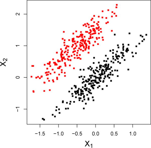
Marginally, X₁ and X₂ discriminate poorly between the groups, but perfect separability is attained when X₁ and X₂ are considered jointly.

The goal of MVPA is often two-fold: (i) to understand underlying mechanisms and patterns in the brain that characterize a disease, and (ii) to develop sensitive and specific image-based biomarkers for disease diagnosis, the prediction of disease progression, or prediction of treatment response. In this work, we elucidate subtle differences between these two goals and provide guidance for future implementation of MVPA in neuroimaging studies. The differences between these goals and the corresponding analyses are directly related to the idea of modeling for the purposes of explanation, description, or prediction as discussed by Shmueli [56]. In this work, we discuss and apply these ideas in the context of MVPA for analyzing neuroimaging data.

Confounding by non-imaging variables such as age and gender can have undesirable effects on the output of MVPA. We show using simulated and real data how confounding of the disease, image relationship may lead to identification of false disease patterns and spurious results. Thus, confounding can undermine the goals of MVPA. We discuss the implications of “regressing out” confounding effects using voxel-wise linear models and propose an alternative based on inverse probability weighting.

The structure of this paper is the following. Section 2 provides a brief review of the use of MVPA in neuroimaging with examples of its implementation in various disease applications. In particular, we focus on the use of the support vector machine (SVM) as a tool for MVPA. In Section 3, we distinguish the target parameters associated with goals (i) and (ii) above and discuss how an analysis must reflect the primary goal. Additionally, we address the issue of confounding by reviewing current practice in imaging and proposing an alternative approach. In Section 4, we illustrate the issues discussed in Section 3 using simulated data. Section 5 presents an application of the methods to data from an Alzheimer’s disease neuroimaging study. We conclude with a discussion in Section 6.

2 Multivariate Pattern Analysis in Neuroimaging

A popular MVPA tool used by the neuroimaging community is the support vector machine (SVM) [7, 27, 60]. This choice is partly motivated by the fact that SVMs are known to work well for high dimension, low sample size data [54]. Often, the number of voxels in a single MRI can exceed one million depending on the resolution of the scanner and the protocol used to obtain the image. The SVM is trained to predict disease class from the vectorized set of voxels that comprise an image. In general, feature weights are taken to describe the contribution of each voxel to the classification function. Alternatives include penalized logistic regression [59] as well as functional principal components and functional partial least squares [46, 66]; additionally, unsupervised methods are gaining ground. Henceforth, we focus on MVPA using the SVM.

We introduce SVMs by supposing that outcome-feature pairs exist of the form ${(y_i,x_i)}_{i=1}^n$, where y_i ∈ {−1, 1} and x_i ∈ ℝ^p for all i = 1,…,n. The hard-margin linear SVM solves the contrained optimization problem

$$\begin{array}{l}\arg \underset{v,b}{\min }\frac{1}{2}{\Vert v\Vert }^2\\ \text{such that}{y}_i(v^{\top }{x}_i+b)\ge 1\forall i=1,\dots ,n,\end{array}$$ (1)

where v ∈ ℝ^p and b ∈ ℝ. When the data are not linearly separable, the soft-margin SVM allows classification errors to be made during training through the use of slack variables ξ_i with associated penalty parameter C. In this case, the optimization problem becomes

$$\begin{array}{l}\arg \underset{v,b,\xi }{\min }\frac{1}{2}{\Vert v\Vert }^2+C{\displaystyle \sum _{i=1}^n{\xi }_i}\\ \text{such that}:\\ y_i(v^{\top }{x}_i+b)\ge 1-{\xi }_i\forall i=1,\dots ,n\\ {\xi }_i\ge 0\forall i=1,\dots ,n,\end{array}$$ (2)

where C ∈ ℝ is a tuning parameter, and ξ ∈ ℝⁿ consists of elements ξ_i. However, in high-dimensional problems where the number of features is greater than the number of observations, the data are always seperable by a linear hyperplane [42]. Thus, MVPA is often applied using the hard-margin SVM in (1) with a linear kernel. For example, this is the approach implemented by: Bendfeldt et al. [3] to classify subgroups of multiple sclerosis patients; Cuingnet et al. [10] and Davatzikos et al. [11] in Alzheimer’s disease applications; and Liu et al. [38], Gong et al. [25], and Costafreda et al. [8] for various classification tasks involving patients with depression. This is only a small subset of the relavant literature, which illustrates the widespread popularity of the approach.

3 MVPA and the Role of Confounding

Let D ∈ {0, 1} be an indicator of disease; let A ∈ ℝ^r denote a vector of non-image covariates; and let X ∈ ℝ^p denote a vectorized image with p voxels. Upper-case letters denote random variables and lower-case letters denote observed data. Suppose D and A both affect X. For example, Alzheimer’s disease is associated with atrophy in the brain that is manifested in structural MRIs, and age is a non-image covariate that also affects brain structure.

Before discussing the role of confounding in MVPA, we comment on a subtlety of the approach that we refer to as “marginal versus joint MVPA.” The issue is simply whether one is interested in estimating disease patterns marginally across non-imaging variables such as age and gender, or jointly with these variables. Suppose data arise from P₀(X,D,A), the joint distribution of X, D, and A, where P₀ has the property that P₀(D | A) = P₀(D). That is, P₀(X,D,A) = P₀(X | D,A)P₀(D)P₀(A). We define the target parameters of both marginal and joint MVPA in terms of P₀(X,D,A) as follows. Let ${\mathcal{C}}_J$ denote a set of classifiers c_J : (x,a) → {−1, 1} that map observed input X = x and A = a to a predicted class c_J(x, a) ∈ {−1, 1}. Define ℒ (y, y′) to be a loss function that penalizes misclassification such as squared error loss, (y – y′)². Let $c_J^{\ast }\in {\mathcal{C}}_J$ be the solution to

$$\underset{c_J\in {\mathcal{C}}_J}{\min }{E}_0[\mathcal{L}\{c_J(X,A),D\}],$$ (3)

where E₀ denotes expectation with respect to P₀. Thus, $c_J^{\ast }$ is a classifier in the set ${\mathcal{C}}_J$ that minimizes the expected loss under P₀; we define $c_J^{\ast }$ to be the target parameter in joint MVPA. Similarly, let ${\mathcal{C}}_M$ denote a set of classifiers c_M : x →{−1, 1} that map observed input X = x to a predicted class c_M (x) ∈{−1, 1}. Let $c_M^{\ast }\in {\mathcal{C}}_M$ be the solution to

$$\underset{c_M\in {\mathcal{C}}_M}{\min }{E}_0[\mathcal{L}\{c_M(X),D\}],$$ (4)

where E₀ denotes expectation with respect to P₀. Thus, $c_M^{\ast }$ is a classifier in the set ${\mathcal{C}}_M$ that minimizes the expected loss under P₀; we define $c_M^{\ast }$to be the target parameter in marginal MVPA.

It follows directly that

$$\underset{c_J\in {\mathcal{C}}_J}{\min }{E}_0[\mathcal{L}\{c_J(X,A),D\}]\le \underset{c_M\in {\mathcal{C}}_M}{\min }{E}_0[\mathcal{L}\{c_M(X),D\}]$$ (5)

because ${\mathcal{C}}_J$ is a larger class than ${\mathcal{C}}_M$. As a concrete example, suppose ${\mathcal{C}}_J$ is chosen to be the set of all linear classifiers so that c_J(X,A) has the form $\text{sign}(b+v_x^{\top }X+v_a^{\top }A)$, where b, v_x, v_a are unknown parameters to be estimated using training data. Similarly, suppose ${\mathcal{C}}_M$ is chosen to be the set of all linear classifiers so that c_M(X) has the form $\text{sign}(b+u_x^{\top }X)$, where b, u_x are unknown parameters to be estimated using training data. Then,

$$\underset{c_J}{\min }{E}_0[\mathcal{L}\{c_J(X,A),D\}]=\underset{b,v_x,v_a}{\min }{E}_0[\mathcal{L}\{\text{sign}(b+v_x^{\top }X+v_a^{\top }A),D\}],$$ (6)

and

$$\begin{array}{l}\underset{c_M}{\min }{E}_0[\mathcal{L}\{c_M(X),D\}]=\underset{b,u_x}{\min }{E}_0[\mathcal{L}\{\text{sign}(b+u_x^{\top }X),D\}]\\ \underset{b,v_x,v_a}{=\min }{E}_0[\mathcal{L}\{\text{sign}(b+v_x^{\top }X+v_a^{\top }A),D\}]\\ \text{subject to}{v}_a=0.\end{array}$$ (7)

Conclude that (5) holds because the minimization in (7) is over a smaller set than that of (6).

Thus, if both training and test data arise from P₀, it is beneficial to perform joint MVPA in terms of expected loss. In other words, if non-imaging variables A are associated with the image X in a way that is informative of disease, it might be of interest to estimate disease patterns jointly with non-imaging variables. In this case, the resulting estimated weight pattern would offer insight to the relative contribution of image features versus demographic and other clinical variables to the discriminative rule. On the other hand, if the research aim is to strictly evaluate the contribution of an image to discrimination, one could perform marginal MVPA.

3.1 MVPA for Descriptive Aims

When the goal of MVPA is to understand patterns of change in the brain that are attributable to a disease, the ideal dataset would contain two images for each subject: one where the subject has the disease and another at the same point in time where the subject is healthy. Of course, this is the fundamental problem of causal inference, as it is impossible to observe both of these potential outcomes [30, 52]. In addition, confounding of the image-disease relationship presents challenges. Figure 2 depicts confounding of the D, X relationship by a single confounder, A. Training a classifier in the presence of confounding may lead to biased estimation of the underlying disease pattern, regardless of whether marginal or joint MVPA is performed. This occurs when classifiers rely heavily on regions that are strongly correlated with confounders instead of regions that encode subtle disease changes [37]. Failing to address confounding in MVPA can lead to a false understanding of image features that characterize the disease. For the remainder of this section, we consider the context of marginal MVPA, but the ideas extend easily to joint MVPA. To simplify notation we abbreviate c_M and ${\mathcal{C}}_M$ as c and $\mathcal{C}$, respectively. In addition, we use the phrase “no confounding” to mean D is independent of A marginally across X, i.e., pr(D | A) = pr(D).

Figure 2.

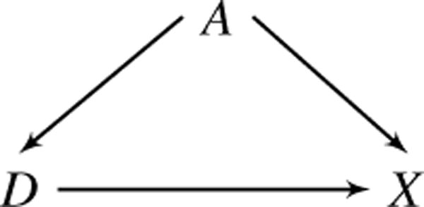
The relationship between D (disease) and X (image) is confounded by A (e.g., age), which affects both D and X.

The target parameter is defined in terms of P₀(X,D,A), the joint distribution of X, D, and A under no confounding. Let $\mathcal{C}$ denote a set of classifiers c : x → {−1, 1} that map observed input vector X = x to a predicted class c(x) ∈ {−1, 1}. As in the previous section, ℒ(y,y′) is a loss function that penalizes misclassification. Let $c_{\ast }\in \mathcal{C}$ be the solution to

$$\underset{c\in \mathcal{C}}{\min }{E}_0[\mathcal{L}\{c(X),D\}],$$ (8)

where E₀ denotes expectation with respect to P₀. Thus, c^* is a classifier in the set $\mathcal{C}$ that minimizes the expected loss under no confounding. For a given set $\mathcal{C}$, the classifier c^∗ is our target parameter. The problem is that in the context of confounding, the observed data are n independent and identically distributed training vectors (Xi,D_i,A_i) sampled from some other joint distribution, say P(X,D,A), instead of P₀(X,D,A).

To illustrate the effects of confounding, consider a toy example with a single confounder A, two features X₁ and X₂, and a binary outcome D. In Alzheimer’s disease, A might be age, D an indicator of disease, and X₁ and X₂ gray matter volumes of two brain regions. We generate N = 1,000 independent observations from the generative model

$$\begin{array}{ccc}\hfill X_1=5-2D+{\epsilon }_1,& & X_2=-5A-0.5D-4AD+{\epsilon }_2,\hfill \\ \hfill A~\text{Unif}[0,1],& & D~\text{Unif}\{-1,1\}\hfill \\ \hfill \left(\begin{array}{c}{\epsilon }_1\\ {\epsilon }_2\end{array}\right)& ~& \text{Normal}\left\{\left(\begin{array}{c}0\\ 0\end{array}\right),\left(\begin{array}{cc}3& 1\\ 1& 3\end{array}\right)\right\}.\hfill \end{array}$$ (9)

Note that (9) has the property that P(D|A) = P(D) so that data generated from this model have joint distribution P₀(X,D,A). The data are plotted in the top three panels of Figure 3 and the linear SVM decision boundary learned from the sample is drawn in gray in the top right panel. Next, we take a biased sample of size n = 400 from the original training observations to induce confounding. In the biased sample, A mimics the confounding effect of age in Alzheimer’s disease in two ways: (i) we give larger values of A a higher probability of being sampled with D = 1, and (ii) A has a decreasing linear effect on the expected value of X₁ and X₂ as displayed in Figure 3. The target parameter is the gray line in the top right panel, which is the SVM decision boundary learned from the features X₁ and X₂ in the unconfounded data. The decision boundary learned from the confounding-induced sample is shown in black in the bottom right panel. Confounding by A shifts the decision boundary and obscures the true relationship between features X₁ and X₂.

Figure 3.

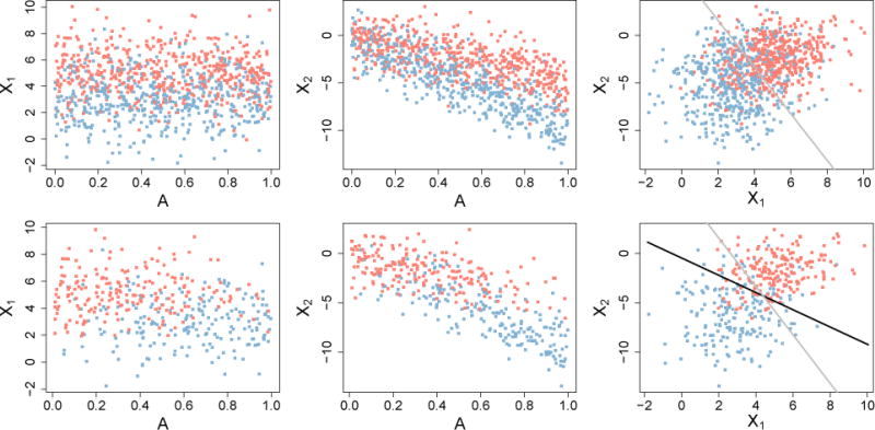
Top row: unconfounded data generated from Model (9). Bottom row: biased-sample data with X₁, X₂, D relationship confounded by A. The target parameter is the SVM boundary learned from the data in the top right plot, shown in gray. The black line is the SVM boundary learned from the confounded sample in the bottom right plot.

There is some variation in the definition of confounding in the imaging literature, making it unclear in some instances if, when, and why an adjustment is made. For example, [18] recommend correcting images for age effects even after age-matching patients and contols. In an age-matched study, age is not a confounder and adjusting for its relationship with X is unnecessary. To address confounding, one approach proposed in the imaging literature is to “regress-out” the effects of confounders from the image X. This is commonly done by fitting a (usually linear) regression of voxel on confounders separately at each voxel and subtracting off the fitted value at each location [18, 22]. The resulting “residual image” is then used in MVPA. Formally, the following model is fit using least squares, separately for each j = 1,…, p:

$$X_j={\beta }_{0,j}+{\beta }_{1,j}^{\top }A+{\epsilon }_j,$$ (10)

where A is now a vector of potential confounders. The least squares estimates ${\widehat{\beta }}_{0,j}$ and ${\widehat{\beta }}_{1,j}$ define the j^th residual voxel,

$${\stackrel{\sim }{X}}_j=X_j-({\widehat{\beta }}_{0,j}+{\widehat{\beta }}_{1,j}^{\top }A).$$

Combining all residuals gives the vector $\stackrel{\sim }{X}=({\stackrel{\sim }{X}}_1,{\stackrel{\sim }{X}}_2,\dots ,{\stackrel{\sim }{X}}_p)$ which is used as the feature vector in the MVPA classifier. We henceforth refer to this method as the adjusted MVPA.

A similar procedure is to fit model (10) using the control group only [18]. We refer to this approach as the control-adjusted MVPA. Let ${\widehat{\beta }}_{0,j}^c$ and ${\widehat{\beta }}_{1,j}^c$ denote the least squares estimates of β_0,j and β_1,j when model (10) is fit using only control-group data. The control-group adjusted features used in the MVPA classifier are then ${\stackrel{\sim }{X}}^c=({\stackrel{\sim }{X}}_1^c,{\stackrel{\sim }{X}}_2^c,\dots ,{\stackrel{\sim }{X}}_p^c)$, where ${\stackrel{\sim }{X}}_j^c=X_j-({\widehat{\beta }}_{0,j}^{c\top }+{\widehat{\beta }}_{1,j}^{c\top }A)$.

A comparison of the adjusted and control-adjusted MVPA features is displayed in Figure 4. Model (9) was used to generate the data and a biased subsample was taken to induce confounding of the X₁, D relationship by A. The first two plots of Figure 4 display original feature X₂ and the adjusted MVPA feature, ${\stackrel{\sim }{X}}_2$. The residuals ${\stackrel{\sim }{X}}_2$ are orthogonal to A across D by definition of least squares residuals. However, marginal separability of the classes on ${\stackrel{\sim }{X}}_2$ is much less than marginal separabilty of the classes on the original feature X₂. This implies that using adjusted features for marginal MVPA may have undesirable consequences on discrimination accuracy and the estimated disease pattern. The right two plots in Figure 4 show that the contol-adjusted MVPA fails to remove the association between X₂ and A. That is, higher ${\stackrel{\sim }{X}}_2^c$ values correspond to lower values of A and lower values of ${\stackrel{\sim }{X}}_2^c$ correspond to higher values of A. Thus, Figure 4 suggests that regression-based methods for addressing confounding are ineffective, motivating our proposed method described next.

Figure 4.

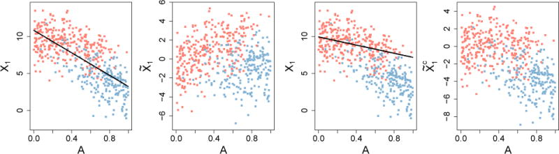
Comparison of adjusted and control-adjusted MVPA features. Left to right: original X₂ with estimated age effect; residuals, ${\stackrel{\sim }{\mathrm{X}}}_2$; original X₂ with contol-group estimated age effect; residuals, ${\stackrel{\sim }{\mathrm{X}}}_2^c$. Lines are the least squares fit of feature on A using the full and control data, respectively.

3.1.1 Inverse Probability Weighted Classifiers

Having formally defined the problem of confounding in MVPA, we now propose a general solution based on inverse probability weighting (IPW) [6, 29, 49, 50]. We show how weighting observations by the inverse probability of D given A recovers an estimate of the objective function in problem (8) when data are sampled from P(X,D,A) rather than P₀(X,D,A). The idea of weighting observations for classifier training is not new, and applying IPW in this way is directly comparable to using sample selection weights to address dataset shift, a well-established concept in the machine learning literature [see, for example: 40, 44, 65]. Similar versions of the following argument can be found in many papers on dataset shift, but we include it here for completeness. We work in the context of marginal MVPA, but the ideas extend directly to joint MVPA.

The expectation in problem (8) can be written as

$$E_0[\mathcal{L}\{c(X),D\}]={\displaystyle \int \mathcal{L}\{c(X),D\}d{P}_0(X,D,A)}.$$ (11)

In the context of confounding, data are sampled not from P₀(X,D,A), but instead from P(X,D,A). Training a classifier using a sample of data from P(X,D,A) targets the objective function

$$E[\mathcal{L}\{c(X),D\}]={\displaystyle \int \mathcal{L}\{c(X),D\}dP(X,D,A)}$$ (12)

rather than expression (11). The right hand side of (12) is equivalent to

$${\displaystyle \int {\displaystyle \int {\displaystyle \int \mathcal{L}\{c(X),D\}dP(X|D,A)dP(D|A)dP(A)}.}}$$ (13)

Define w = dP(D | A)=pr(D = 1 | A)𝟙_D=1+pr(D=−1|A)𝟙_D=−1. Then, expression (13) can be written as

$${\displaystyle \int {\displaystyle \int {\displaystyle \int w\mathcal{L}\{c(X),D\}dP(X|D,A)dP(A)}.}}$$ (14)

Note that the “unconfounded” population distribution P₀(X,D,A) may not be unique because thus far we have not restricted P₀(A) P₀(D) in any way. Henceforth, we assume P₀(A) = P(A), i.e., the marginal distribution of confounders from which the observed sample was drawn. We also assume dP₀(X | D,A) = dP(X | D,A), meaning the distribution of the image is the same in both populations conditional on disease status and non-imaging variables. In addition, let pr₀(D = d) denote the marginal probability of observing D = d under P₀(X,D,A). Without loss of generality, assume pr₀(D = 1) = pr₀(D = −1) = 1/2, corresponding to a hypothetical balanced population where each patient’s two potential outcomes, one under disease presence and one under absence of disease, are observed. Then, under these assumption and noting that dP₀(D | A) = dP₀(D) = pr₀(D = 1)𝟙_D=1+pr₀(D = −1)𝟙_D=0 = 1/2, expression (14) can be written as

$${\displaystyle \int {\displaystyle \int {\displaystyle \int w\mathcal{L}\{c(X),D\}d{P}_0(X|D,A)d{P}_0(A)\propto E_0[w\mathcal{L}\{c(X),D\}]}.}}$$

Thus, we have shown that E[ℒ {c(X),D}] ∝ E₀[wL {c(X),D}], and hence

$$\underset{c\in \mathcal{C}}{\min }E\left[\frac{1}{w}\mathcal{L}\{c(X),D\}\right]=\underset{c\in \mathcal{C}}{\min }{E}_0[\mathcal{L}\{c(X),D\}].$$ (15)

In practice, the inverse probability weights are often unknown and must be estimated from the data. One way to estimate the weights is by positing a model and obtaining fitted values for the probability of disease given confounders A, also known as the propensity score [2, 51]. Logistic regression is commonly used to model the propensity score, however, more flexible approaches using machine learning have also received attention [36]. Using logistic regression, the model would be specified as

$$\text{logit}[\text{pr}(D=1|A)]={\gamma }_0+A^{\top }{\gamma }_1.$$

Then, the estimated inverse probability weights would follow as

$${\widehat{w}}_i^{-1}={[{\mathrm{𝟙}}_{D_i=1}\mathrm{expit}(\widehat{{\gamma }_0}+A_i^{\top }\widehat{{\gamma }_1})+{\mathrm{𝟙}}_{D_i=0}\{1-\text{expit}(\widehat{{\gamma }_0}+A_i^{\top }\widehat{{\gamma }_1}))\}]}^{-1},$$

where expit(x) is the inverse of the logit function, expit(x) = e^x/(1 + e^x).

Inverse probability weighting (IPW) can be naturally incorporated into some classification models such as logistic regression. Subject-level weighting can be accomplished in the soft-margin SVM framework defined in expression (16) by weighting the slack variables. Suppose the true weights w_i are known. To demonstrate how IPW can be incorporated in the soft-margin SVM, we first consider approximate weights, T_i, defined as subject i’s inverse probability weight rounded to the nearest integer. For example, suppose subject i’s inverse weight is 1/w_i = 3.2; then, T_i = 3. Next, consider creating an approximately balanced psuedo-population which consists of T_i copies of each original subject’s data, i = 1,…,n. This psuedo-population therefore has $n\ast ={\displaystyle {\sum }_{i=1}^n{T}_i}$ observations. The soft-margin SVM in the psuedo-population is then

$$\begin{array}{l}\arg \underset{v,b,\xi \ast }{\min }\frac{1}{2}{\Vert v\Vert }^2+C{\displaystyle \sum _{j=1}^{n\ast }{\xi }_j^{\ast }}\\ \text{such that}:\\ y_j^{\ast }(v^{\top }{x}_j^{\ast }+b)\ge 1-{\xi }_j^{\ast }\forall j=1,\dots ,n\ast \\ {\xi }_j^{\ast }\ge 0\forall j=1,\dots ,n.\end{array}$$

However, in the approximately balanced population, some of the $(y_j^{\ast },x_j^{\ast })$ pairs are identical copies which implies some of the constraints are redundant. For example, $(y_1^{\ast },x_1^{\ast })$ and $(y_2^{\ast },x_2^{\ast })$ are identical copies that correspond to (y₁,x₁) in the original sample. Then it can be seen that ${\xi }_1^{\ast }={\xi }_2^{\ast }$ must hold in (16). Let ${\xi }_1={\xi }_1^{\ast }={\xi }_2^{\ast }$. Then, the constraints

$$\begin{array}{l}{y}_1^{\ast }(v^{\top }{x}_1^{\ast }+b)\ge 1-{\xi }_1^{\ast }\\ y_2^{\ast }(v^{\top }{x}_2^{\ast }+b)\ge 1-{\xi }_2^{\ast }\\ {\xi }_1^{\ast }\ge 0\\ {\xi }_2^{\ast }\ge 0\end{array}$$

in (16) are equivalent to

$$\begin{array}{l}{y}_1(v^{\top }{x}_1+b)\ge 1-{\xi }_1\\ {\xi }_1\ge 0\end{array}$$

In fact, assuming all observations in the original n samples are unique, there are n unique constraints of the form $y_i(v^{\top }{x}_i+b)\ge 1-{\xi }_i$ and ξ_i ≥ 0, corresponding to the original i = 1,…,n samples. In addition, it is easy to show that ${\displaystyle {\sum }_{j=1}^{n\ast }{\xi }_j^{\ast }}={\displaystyle {\sum }_{i=1}^n{T}_i{\xi }_i}$. Thus, (16) is equivalent to the original data soft-margin SVM with weighted slack variables in the objective function:

$$\begin{array}{l}\arg \underset{v,b,\xi }{\min }\frac{1}{2}{\Vert v\Vert }^2+C{\displaystyle \sum _{i=1}^n{T}_i{\xi }_i}\\ \text{such that}:\\ y_i(v^{\top }{x}_i+b)\ge 1-{\xi }_i\forall i=1,\dots ,n\\ {\xi }_i\ge 0\forall i=1,\dots ,n.\end{array}$$ (16)

The previous argument suggests one could use the w_i rather than the truncated versions, T_i. However, to our knowledge there does not exist an implementation of the SVM in R [45] that enables weighting the slack variables at the subject level. Implementation of subject-level weighting is available in the library libSVM [5]. Practitioners familiar with MATLAB or Python can implement the weighted SVM directly or by calling one of these languages from R using a tool such as the “rPython” package (http://rpython.r-forge.r-project.org/). We are currently working on an R implementation of the IPW-SVM. In the meantime, we propose an approximation based on the truncated inverse weights for practitioners who are only familiar with R. The full details of our proposed algorithm are presented below. We implemented the following algorithm in Section 4 using the package “e1071” in R.

Approximate IPW Algorithm for SVMs

1. Estimate the propensity scores for each subject in the training data. For example, we might posit the logistic regression model,

   $$\text{logit}\{\text{pr}(D_i=1|A_i)\}={\gamma }_0+{\gamma }_1^{\top }{A}_i$$

   and estimate the parameters using standard software. Denote the estimated probabilities by $\widehat{\text{pr}}(D_i=1|A_i)$ for i = 1,…,n.
2. Let $\widehat{T_i}$ denote the estimated inverse probability weight for subject i, truncated to the nearest integer. For example, if subject i has

   $$\widehat{w_i}=\mathrm{𝟙}(D_i=1)\widehat{\text{pr}}(D_i=1|A_i)+\mathrm{𝟙}(D_i=0)\widehat{\text{pr}}(D_i=0|A_i)=0.35,$$

   then $\widehat{T_i}=3$.

3. Create an augmented sample of size ${\displaystyle {\sum }_{i=1}^n\widehat{T_i}}$ that consists of $\widehat{T_i}$ repeated observations of the original data from subject i.

4. Train the SVM classifier using the augmented sample from Step 3.

The augmented sample approximates a sample of data from P₀(X,D,A). The IPW-SVM algorithm only works when the data are not linearly separable. Otherwise, there are no slack variables in the optimization problem to weight. To provide intuition, suppose we are trying to separate two points in two-dimensional space. The optimization problem is then the hard-margin SVM formulation:

$$\begin{array}{l}\arg \underset{v,b}{\min }\frac{1}{2}{\Vert v\Vert }^2\\ \text{such that}:\\ y_1(v^{\top }{x}_1+b)=1,\\ y_2(v^{\top }{x}_2+b)=1.\end{array}$$

Adding copies of the data only adds redundant constraints that do not affect the optimization at all. This is a major issue in neuroimaging because the data often have more features than observations and are thus linearly separable. When p ≥ n, we propose the following approach based on principal component analysis.

Approximate IPW-PCA Algorithm for SVMs

1. Perform Steps 1–3 of the Approximate IPW Algorithm for SVMs.

2. Let Z denote the n^∗ × p psuedo-population feature matrix with columns corresponding to (imaging) features and rows corresponding to $\widehat{T_i}$ copies of subject i’s original data for i = 1,…,n. Obtain the first several principal component scores from the eigen-decomposition of Z^⊤Z which explain a prespecified proportion of variation in the psuedo-population data.

3. Train the SVM classifier using the principal component scores obtained from the augmented sample. This sample approximates a sample of principal component scores arising from P₀(X,D,A).

Unfortunately, the resulting weights no longer enjoy the same interpretability as the weights from a SVM that inputs the features directly. The weights now correspond to linear combinations of voxels or regions that are discriminative rather than the individual voxels or regions. We are currently exploring alternatives to address confounding when p ≥ n that retain the original interpretability of the features.

To summarize the main points in this section, Figure 5 provides a decision tree with recommended analysis plans for given data structures and scientific aims that are applicable when p < n. We believe tools such as Figure 5 may be useful to help initiate or guide discussion with collaborators about the design and analysis of future neuroimaging studies.

Figure 5.

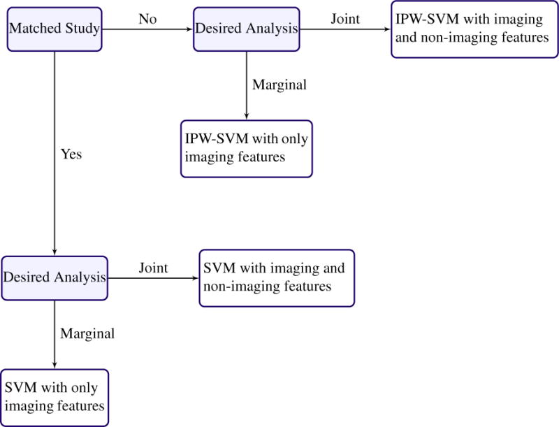
Recommended analysis plan for estimating disease patterns when the data have more observations than features.

3.2 Remark on MVPA for Biomarker Development

In constrast to being potential confounders that bias results in the previous section, non-imaging variables play a different, and advantageous, role when MVPA is used to develop biomarkers for disease diagnosis, progression, or treatment response. It is unlikely that the true underlying distribution of non-imaging variables such as age is balanced with respect to disease. That is, it is unlikely a matched study is representative of the population to which a derived biomarker will be applied. As a result, matched studies or IPW methods that create balance with respect to the disease and non-imaging variables may not result in the optimal classifier or biomarker. This observation has been made previously in different contexts, including the in the statistical literature [32] and the machine learning literature [40, 44].

In machine learning, dataset shift is the phenomenon where the joint distribution of training data differs from the data distribution where the classifier will be applied [40, 44]. Covariate shift is a special case of dataset shift which corresponds to a shift in the feature distribution used to obtain predictions from the classification model. Solutions usually involve some version of observation weighting or moment matching to make the training and test feature distributions more comparable [4, 26, 31, 55, 57, 58]. Applying dataset shift methods to neuroimaging data has the potential to improve biomarker effectiveness and generalizability. For example, suppose a biomarker is developed using imaging and demographic data from a matched study. That is, patients have been selected so that there are equal numbers of cases and controls for all values of the demographic variables. However, suppose it is known that in the general population the disease is more prevalent in older patients. Then, the matched study data and the population to which the biomarker will be applied come from different joint distributions. Covariate shift methods enable prior knowledge of the population distribution to be leveraged to attain better predictive performance of the biomarker. Figure 6 provides a decision tree with recommended analysis plans when p < n and the scientific aim of MVPA is to optimize predictive performance.

Figure 6.

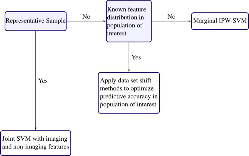
Recommended anaylsis plan for optimizing predictive performance, possibly for the purpose of biomarker development, when the data have more observations than features.

4 Simulations

In this section we evaluate the finite sample performance of the approximate IPW-SVM relative to the regression methods discussed in Section 3.1. We simulate training data from the following generative model:

$$\begin{array}{ccc}\hfill X_1=5-2D+{\epsilon }_1,& & X_2=-5A-0.5D-4AD+{\epsilon }_2,\hfill \\ \hfill A~\text{Unif}[0,1],& & D~\text{Unif}\{-1,1\}\hfill \\ \hfill \left(\begin{array}{c}{\epsilon }_1\\ {\epsilon }_2\end{array}\right)& ~& \text{Normal}\{\left(\begin{array}{c}0\\ 0\end{array}\right),(\begin{array}{cc}3& 1\\ 1& 3\end{array}\left)\right\},\hfill \end{array}$$ (17)

in which A is not a confounder because it does not affect D. This is the same model used for the toy examples in Section 3.1. For each of M = 10,000 iterations, we first generate a sample of size N = 1,000 from model (17) and train two SVMs: (i) a marginal SVM with only X₁ and X₂ as features, and (ii) a joint SVM with X₁, X₂, and A included as a features. The weight patterns from these are regarded as the target parameters for our comparisons. Next we induce confounding by taking a biased subsample of size n = 400 from the unconfounded training data. We apply two marginal methods to the biased sample: the marginal unadjusted SVM and the marginal IPW-SVM. In addition, we apply six joint methods to the biased sample: the joint unadjusted SVM, the adjusted SVM with and without A as a feature, the control-adjusted SVM with and without A as a feature, and the joint IPW-SVM. The adjusted and control-adjusted SVM are regression-based methods commonly used in the neuroimaging literature that are described in Section 3.1.

We use L₂ distance between the weight vectors as one critera for comparison. Additionally, we note that the solution to optimization problem (8) in Section 3, which we define as our target parameter for a joint analysis, acheives optimal test accuracy in the unconfounded population among joint MVPA methods. Similarly, the solution to optimization problem (4) in Section 3, which we define as our target parameter for a marginal analysis, acheives optimal test accuracy in the unconfounded population among marginal MVPA methods. Thus, at each iteration we also generate a test data set of size S = 1,000 from model (17) in order to compare the test accuracy of all the methods. We expect methods that attain weight patterns closest to the corresponding true weight pattern will also attain the highest test accuracies. Results are presented separately for marginal and joint MVPA below.

4.1 Marginal MVPA Results

As noted in Section 3.1, the adjusted and control-adjusted SVMs are not marginal methods because they indirectly incorporate information about A in the regression-adjusted image features. Thus, in this section we compare only the approximate IPW-SVM to the unadjusted SVM which trains on the original data without addressing confounding. Figure 7 displays boxplots of the average test accuracy and average L₂ distance from the true weights for M = 10,000 iterations. The IPW-SVM attains nearly optimal average test accuracy and performs much better than the unadjusted SVM in terms of average L₂ distance. Finally, we looked at the percentage of iterations where the true order of the absolute value of the weights was correctly estimated. The IPW-SVM returns the correct pattern of feature importance 93% of the time, in comparison to a dismal 1% by the unadjusted SVM. The poor performance of the unadjusted SVM is due to its reliance on the false separability caused by the confounded relationship between D and A.

Figure 7.

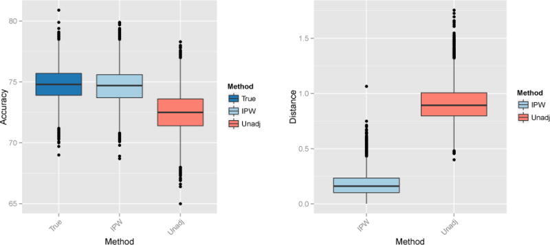
Left: Percent test accuracy of the true and estimated SVM decision rules from the marginal MVPA methods. Right: L₂ distance between the true and estimated weight vectors from the marginal MVPA methods.

4.2 Joint MVPA Results

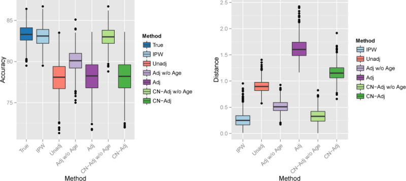
In this section we compare all joint MVPA methods to the joint IPW-SVM. Figure 8 displays boxplots of the average test accuracy and average L₂ distance from the true weights for M = 10,000 iterations. The IPW-SVM again attains nearly optimal average test accuracy. The control-adjusted SVM without age as a feature performs second-best on average. In terms of average L₂ distance, the IPW-SVM and control-adjusted SVM without age perform approximately the same and outperform all other methods on average.

Figure 8.

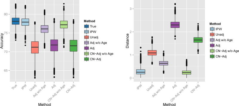
Left: Percent test accuracy of the true and estimated SVM decision rules from the joint MVPA methods. Right: L₂ distance between the true and estimated weight vectors from the marginal MVPA methods.

In some cases, the IPW-SVM outperforms the control-adjusted SVM. To demonstrate, we repeated the joint MVPA replacing X₁ and X₂ in model (9) with

$$X_1=5-3D+{\epsilon }_1,X_2=-3A-4D+3AD+{\epsilon }_2.$$

Results are displayed in Figure 9. The IPW-SVM performs best on average in terms of prediction accuracy and L₂ distance between the true and estimated weights.

Figure 9.

Left: Percent test accuracy of the true and estimated SVM decision rules from the joint MVPA methods. Right: L₂ distance between the true and estimated weight vectors from the marginal MVPA methods.

5 Application

The Alzheimer’s Disease Neuroimaging Initiative (ADNI) (http://www.adni.loni.usc.edu) is a $60 million study funded by public and private resources including the National Institute on Aging, the National Institute of Biomedical Imaging and Bioengineering, the Food and Drug Administration, private pharmaceutical companies, and non-profit organizations. The goals of the ADNI are to better understand progression of mild cognitive impairment (MCI) and early Alzheimer’s disease (AD) and to determine effective biomarkers for disease diagnosis, monitoring, and treatment development. MCI is characterized by cognitive decline that does not generally interfere with normal daily function and is distinct from Alzheimer’s disease [24]. However, individuals with MCI are considered to be at risk for progression to Alzheimer’s disease. Thus, studying the development of MCI and factors associated with progression to Alzheimer’s disease is of critical scientific importance.

We apply the IPW-SVM to structural MRIs from the ADNI database. Before performing group-level analyses, each subject’s MRI is passed through a series of preprocessing steps that facilitate between-subject comparability. We implemented a multi atlas segmentation pipeline [17] to estimate the volume of 137 regions of interest (ROIs) in the brain for each subject and divide each region by that subject’s intracranial volume to adjust for differences in individual brain size. The data we use here consist of 204 patients diagnosed with MCI and 178 healthy controls (CN) between the ages of 70 and 80. Neurodegenerative diseases are associated with atrophy in the brain, and thus the MCI group has smaller volumes in particular ROIs on average compared to the CN group. In this analysis, we study the consequences of confounding on a MVPA of the ADNI data which aims to identify multivariate patterns of atrophy associated with MCI.

The ADNI study was matched on confounders such as age and gender. This is advantageous for our analysis because we are able to first train a SVM using the full data to classify MCI versus CN patients. We take the resulting weight pattern as the target parameter. To induce confounding, we take a biased subsample where older MCI patients and younger CNs are more likely to be selected. Results from the unconfounded, full-data SVM are compared to results from six methods that we apply to the confounded subsample: (i) an unadjusted SVM (Unadj) learned from the biased sample with age included as a feature, (ii) the adjusted SVM (Adj) described in Section 3.1 with and without age as a feature, (iii) the control-adjusted SVM (CN-Adj) [18] described in Section 3.1 with and without age as a feature, and (iv) the IPW-SVM described in Section 3.1 with age included as a feature. We repeat this process for 10,000 biased samples and present results averaged over these iterations.

Boxplots of the euclidean distance between the estimated and true weight vectors are shown in Figure 10. The unadjusted, CN-adjusted without age, CN-adjusted with age, and IPW-SVM produce similar results, and these methods reproduce weight patterns closest to the truth when compared to the adjusted SVMs with and without age. The adjusted SVM without age appears unstable. In fact, we truncated the y-axis for better visual comparison of the methods, cutting off over a hundred additional weight distances for the adjusted SVM that exceeded 3.25.

Figure 10.

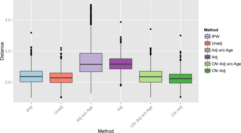
Euclidean distance between the true and estimated weight patterns for all joint MVPA methods using the 137 volumes.

In addition to performing MVPA on the full data, we apply the PCA approach detailed in Section 3.1. To obtain the “true” low-dimensional weight pattern, we perform PCA on only the image features from the full data and retain the first three PC scores. For each of 10,000 iterations, we again take a biased subsample to induce confounding. We compare the unadjusted, adjusted, control-adjusted, and IPW-SVM using only the PC scores as features and using the PC scores with age as features. For the regression-based adjusted SVM and control-adjusted SVM, we perform PCA on the image after regressing out the region-wise age effects. For the IPW-PCA-SVM we follow the algorithm in Section 3.1. Figure 11 provides boxplots of the euclidian distance between the estimated and true weight vectors. On average the IPW-PCA-SVM performs better than the other methods, but several iterations yielded undesirable performance. This is most likely due to occasionally very large estimated inverse probability weights which have large influence on the psuedo-population where the SVM is trianed. Overall, it seems that IPW methods work well in problems with a small number of features and when there is sufficient overlap in the distribution of confounders between the two groups so that the estimated inverse probability weights are stable.

Figure 11.

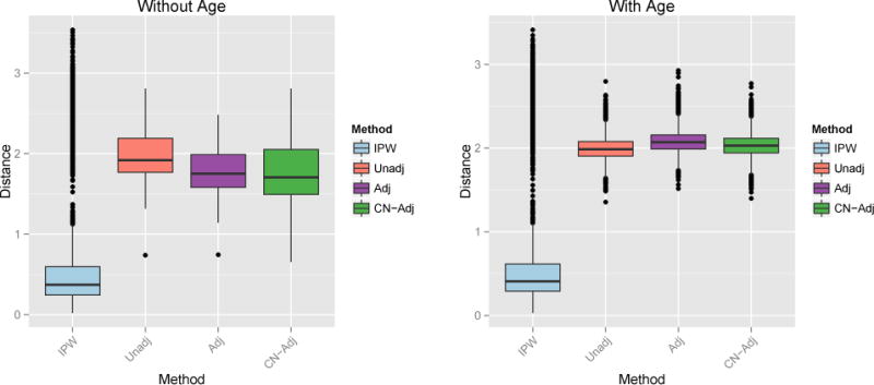
Euclidean distance between the true and estimated weight patterns. Left: First three PC scores as features. Right: First three PC scores and Age as features.

6 Discussion

The IPW framework for MVPA is an intuitive, principled way to address confounding. When applied to classification frameworks in the context of confounding, IPW approaches can identify true underlying patterns associated with disease. We believe there are several advantages to addressing confounding in MVPA using IPW. First, as demonstrated by simulation results, the IPW approach is estimating the actual target parameter of interest, which is to recover disease patterns that are present under no confounding. In addition, a nice implication is that MVPA can be implemented even in unmatched studies. In cases where a matched study is too expensive or otherwise infeasible, IPW methods enable researchers to still perform MVPA and obtain correct and reproducible results. Finally, IPW is simple and intuitive, and the general idea is well-established in the causal inference and statistics communities. Thus, future research aiming to perform inference on the estimated disease patterns can rely on existing theory. We are currently working on extending existing inference methods for MVPA [23] to account for confounding.

Confounding in neuroimaging is a form of class imbalance that depends on non-imaging variables such as age and gender. We have proposed a solution that weights by the conditional probability of class membership given confounders, i.e., inverse probability weighting. It is possible alternative methods for dealing with class imbalance could be extended as well [28].

In high-dimensional problems, we conjecture that confounding may not have as much of an effect on the maximum margin hyperplane of the SVM due to the curse of dimensionality. This might explain why all methods performed similarly on the ADNI data. Further exploring the effects of confounding on high-dimensional classification models is imperative for neuroimaging research and may greatly impact current practice in the field.

References

- 1.Ashburner J, Friston KJ. Voxel-based morphometry – the methods. Neuroimage. 2000;11(6):805–821. doi: 10.1006/nimg.2000.0582. [DOI] [PubMed] [Google Scholar]
- 2.Austin PC. An introduction to propensity score methods for reducing the effects of confounding in observational studies. Multivariate behavioral research. 2011;46(3):399–424. doi: 10.1080/00273171.2011.568786. [DOI] [PMC free article] [PubMed] [Google Scholar]
- 3.Bendfeldt K, Klöppel S, Nichols TE, Smieskova R, Kuster P, Traud S, Mueller-Lenke N, Naegelin Y, Kappos L, Radue EW, et al. Multivariate pattern classification of gray matter pathology in multiple sclerosis. Neuroimage. 2012;60(1):400–408. doi: 10.1016/j.neuroimage.2011.12.070. [DOI] [PubMed] [Google Scholar]
- 4.Bickel S, Brückner M, Scheffer T. Discriminative learning under covariate shift. The Journal of Machine Learning Research. 2009;10:2137–2155. [Google Scholar]
- 5.Chang CC, Lin CJ. LIBSVM: A library for support vector machines. ACM Transactions on Intelligent Systems and Technology. 2011;2:27:1–27:27. [Google Scholar]
- 6.Cole SR, Hernán MA. Constructing inverse probability weights for marginal structural models. American journal of epidemiology. 2008;168(6):656–664. doi: 10.1093/aje/kwn164. [DOI] [PMC free article] [PubMed] [Google Scholar]
- 7.Cortes C, Vapnik V. Support-vector networks. Machine learning. 1995;20(3):273–297. [Google Scholar]
- 8.Costafreda SG, Chu C, Ashburner J, Fu CH. Prognostic and diagnostic potential of the structural neuroanatomy of depression. PLoS One. 2009;4(7):e6353. doi: 10.1371/journal.pone.0006353. [DOI] [PMC free article] [PubMed] [Google Scholar]
- 9.Craddock RC, Holtzheimer PE, Hu XP, Mayberg HS. Disease state prediction from resting state functional connectivity. Magnetic Resonance in Medicine. 2009;62(6):1619–1628. doi: 10.1002/mrm.22159. [DOI] [PMC free article] [PubMed] [Google Scholar]
- 10.Cuingnet R, Rosso C, Chupin M, Lehricy S, Dormont D, Benali H, Samson Y, Colliot O. Spatial regularization of {SVM} for the detection of diffusion alterations associated with stroke outcome. Medical Image Analysis. 2011;15(5):729–737. doi: 10.1016/j.media.2011.05.007. Special Issue on the 2010 Conference on Medical Image Computing and Computer-Assisted Intervention. [DOI] [PubMed] [Google Scholar]
- 11.Davatzikos C, Bhatt P, Shaw LM, Batmanghelich KN, Trojanowski JQ. Prediction of {MCI} to {AD} conversion, via mri, {CSF} biomarkers, and pattern classification. Neurobiology of Aging. 2011;32(12):2322.e19–2322.e27. doi: 10.1016/j.neurobiolaging.2010.05.023. [DOI] [PMC free article] [PubMed] [Google Scholar]
- 12.Davatzikos C, Genc A, Xu D, Resnick SM. Voxel-based morphometry using the {RAVENS} maps: Methods and validation using simulated longitudinal atrophy. NeuroImage. 2001;14(6):1361–1369. doi: 10.1006/nimg.2001.0937. [DOI] [PubMed] [Google Scholar]
- 13.Davatzikos C, Resnick S, Wu X, Parmpi P, Clark C. Individual patient diagnosis of {AD} and {FTD} via high-dimensional pattern classification of {MRI} NeuroImage. 2008;41(4):1220–1227. doi: 10.1016/j.neuroimage.2008.03.050. [DOI] [PMC free article] [PubMed] [Google Scholar]
- 14.Davatzikos C, Ruparel K, Fan Y, Shen D, Acharyya M, Loughead J, Gur R, Langleben DD. Classifying spatial patterns of brain activity with machine learning methods: application to lie detection. Neuroimage. 2005;28(3):663–668. doi: 10.1016/j.neuroimage.2005.08.009. [DOI] [PubMed] [Google Scholar]
- 15.Davatzikos C, Xu F, An Y, Fan Y, Resnick SM. Longitudinal progression of alzheimer’s-like patterns of atrophy in normal older adults: the spare-ad index. Brain. 2009;132(8):2026–2035. doi: 10.1093/brain/awp091. [DOI] [PMC free article] [PubMed] [Google Scholar]
- 16.De Martino F, Valente G, Staeren N, Ashburner J, Goebel R, Formisano E. Combining multivariate voxel selection and support vector machines for mapping and classification of fmri spatial patterns. Neuroimage. 2008;43(1):44–58. doi: 10.1016/j.neuroimage.2008.06.037. [DOI] [PubMed] [Google Scholar]
- 17.Doshi J, Erus G, Ou Y, Gaonkar B, Davatzikos C. Multi-atlas skull-stripping. Academic radiology. 2013;20(12):1566–1576. doi: 10.1016/j.acra.2013.09.010. [DOI] [PMC free article] [PubMed] [Google Scholar]
- 18.Dukart J, Schroeter ML, Mueller K, Initiative TADN. Age correction in dementia – matching to a healthy brain. PLoS ONE. 2011;6(7):e22193. doi: 10.1371/journal.pone.0022193. [DOI] [PMC free article] [PubMed] [Google Scholar]
- 19.Fan Y, Shen D, Gur RC, Gur RE, Davatzikos C. Compare: classification of morphological patterns using adaptive regional elements. Medical Imaging, IEEE Transactions on. 2007;26(1):93–105. doi: 10.1109/TMI.2006.886812. [DOI] [PubMed] [Google Scholar]
- 20.Frackowiak R, Friston K, Frith C, Dolan R, Mazziotta J, editors. Human Brain Function. Academic Press; USA: 1997. [Google Scholar]
- 21.Friston KJ, Frith C, Liddle P, Frackowiak R. Comparing functional (pet) images: the assessment of significant change. Journal of Cerebral Blood Flow & Metabolism. 1991;11(4):690–699. doi: 10.1038/jcbfm.1991.122. [DOI] [PubMed] [Google Scholar]
- 22.Friston KJ, Holmes AP, Worsley KJ, Poline JP, Frith CD, Frackowiak RS. Statistical parametric maps in functional imaging: a general linear approach. Human brain mapping. 1994;2(4):189–210. [Google Scholar]
- 23.Gaonkar B, Davatzikos C. Analytic estimation of statistical significance maps for support vector machine based multi-variate image analysis and classification. NeuroImage. 2013;78(0):270–283. doi: 10.1016/j.neuroimage.2013.03.066. [DOI] [PMC free article] [PubMed] [Google Scholar]
- 24.Gauthier S, Reisberg B, Zaudig M, Petersen RC, Ritchie K, Broich K, Belleville S, Brodaty H, Bennett D, Chertkow H, et al. Mild cognitive impairment. The Lancet. 2006;367(9518):1262–1270. doi: 10.1016/S0140-6736(06)68542-5. [DOI] [PubMed] [Google Scholar]
- 25.Gong Q, Wu Q, Scarpazza C, Lui S, Jia Z, Marquand A, Huang X, McGuire P, Mechelli A. Prognostic prediction of therapeutic response in depression using high-field mr imaging. Neuroimage. 2011;55(4):1497–1503. doi: 10.1016/j.neuroimage.2010.11.079. [DOI] [PubMed] [Google Scholar]
- 26.Gretton A, Smola A, Huang J, Schmittfull M, Borgwardt K, Schölkopf B. Covariate shift by kernel mean matching. Dataset shift in machine learning. 2009;3(4):5. [Google Scholar]
- 27.Hastie T, Tibshirani R, Friedman J. Springer New York Inc. 2001. [Google Scholar]
- 28.He H, Garcia EA. Learning from imbalanced data. Knowledge and Data Engineering, IEEE Transactions on. 2009;21(9):1263–1284. [Google Scholar]
- 29.Hernán MA, Robins JM. Estimating causal effects from epidemiological data. Journal of epidemiology and community health. 2006;60(7):578–586. doi: 10.1136/jech.2004.029496. [DOI] [PMC free article] [PubMed] [Google Scholar]
- 30.Holland PW. Statistics and causal inference. Journal of the American statistical Association. 1986;81(396):945–960. [Google Scholar]
- 31.Huang J, Gretton A, Borgwardt KM, Schölkopf B, Smola AJ. Advances in neural information processing systems. 2006. Correcting sample selection bias by unlabeled data; pp. 601–608. [Google Scholar]
- 32.Janes H, Pepe MS. Matching in studies of classification accuracy: implications for analysis, efficiency, and assessment of incremental value. Biometrics. 2008;64(1):1–9. doi: 10.1111/j.1541-0420.2007.00823.x. [DOI] [PubMed] [Google Scholar]
- 33.Klöppel S, Stonnington CM, Chu C, Draganski B, Scahill RI, Rohrer JD, Fox NC, Jack CR, Ashburner J, Frackowiak RSJ. Automatic classification of mr scans in alzheimer’s disease. Brain. 2008;131(3):681–689. doi: 10.1093/brain/awm319. [DOI] [PMC free article] [PubMed] [Google Scholar]
- 34.Koutsouleris N, Meisenzahl EM, Davatzikos C, Bottlender R, Frodl T, Scheuerecker J, Schmitt G, Zetzsche T, Decker P, Reiser M, et al. Use of neuroanatomical pattern classification to identify subjects in at-risk mental states of psychosis and predict disease transition. Archives of general psychiatry. 2009;66(7):700–712. doi: 10.1001/archgenpsychiatry.2009.62. [DOI] [PMC free article] [PubMed] [Google Scholar]
- 35.Langs G, Menze BH, Lashkari D, Golland P. Detecting stable distributed patterns of brain activation using gini contrast. NeuroImage. 2011;56(2):497–507. doi: 10.1016/j.neuroimage.2010.07.074. [DOI] [PMC free article] [PubMed] [Google Scholar]
- 36.Lee BK, Lessler J, Stuart EA. Improving propensity score weighting using machine learning. Statistics in medicine. 2010;29(3):337–346. doi: 10.1002/sim.3782. [DOI] [PMC free article] [PubMed] [Google Scholar]
- 37.Li L, Rakitsch B, Borgwardt K. ccsvm: correcting support vector machines for confounding factors in biological data classification. Bioinformatics. 2011;27(13):i342–i348. doi: 10.1093/bioinformatics/btr204. [DOI] [PMC free article] [PubMed] [Google Scholar]
- 38.Liu F, Guo W, Yu D, Gao Q, Gao K, Xue Z, Du H, Zhang J, Tan C, Liu Z, et al. Classification of different therapeutic responses of major depressive disorder with multivariate pattern analysis method based on structural mr scans. PLoS One. 2012;7(7):e40968. doi: 10.1371/journal.pone.0040968. [DOI] [PMC free article] [PubMed] [Google Scholar]
- 39.Mingoia G, Wagner G, Langbein K, Maitra R, Smesny S, Dietzek M, Burmeister HP, Reichenbach JR, Schlösser RG, Gaser C, et al. Default mode network activity in schizophrenia studied at resting state using probabilistic ica. Schizophrenia research. 2012;138(2):143–149. doi: 10.1016/j.schres.2012.01.036. [DOI] [PubMed] [Google Scholar]
- 40.Moreno-Torres JG, Raeder T, Alaiz-RodríGuez R, Chawla NV, Herrera F. A unifying view on dataset shift in classification. Pattern Recognition. 2012;45(1):521–530. [Google Scholar]
- 41.Mourão-Miranda J, Bokde AL, Born C, Hampel H, Stetter M. Classifying brain states and determining the discriminating activation patterns: support vector machine on functional mri data. NeuroImage. 2005;28(4):980–995. doi: 10.1016/j.neuroimage.2005.06.070. [DOI] [PubMed] [Google Scholar]
- 42.Orrù G, Pettersson-Yeo W, Marquand AF, Sartori G, Mechelli A. Using support vector machine to identify imaging biomarkers of neurological and psychiatric disease: a critical review. Neuroscience & Biobehavioral Reviews. 2012;36(4):1140–1152. doi: 10.1016/j.neubiorev.2012.01.004. [DOI] [PubMed] [Google Scholar]
- 43.Pereira F. Beyond brain blobs: machine learning classifiers as instruments for analyzing functional magnetic resonance imaging data. 2007. ProQuest. [Google Scholar]
- 44.Quionero-Candela J, Sugiyama M, Schwaighofer A, Lawrence ND. Dataset shift in machine learning. The MIT Press; 2009. [Google Scholar]
- 45.R Core Team. R: A Language and Environment for Statistical Computing. R Foundation for Statistical Computing; Vienna, Austria: 2014. [Google Scholar]
- 46.Reiss PT, Ogden RT. Functional principal component regression and functional partial least squares. Journal of the American Statistical Association. 2007;102(479):984–996. [Google Scholar]
- 47.Reiss PT, Ogden RT. Functional generalized linear models with images as predictors. Biometrics. 2010;66(1):61–69. doi: 10.1111/j.1541-0420.2009.01233.x. [DOI] [PubMed] [Google Scholar]
- 48.Richiardi J, Eryilmaz H, Schwartz S, Vuilleumier P, Van De Ville D. Decoding brain states from fmri connectivity graphs. Neuroimage. 2011;56(2):616–626. doi: 10.1016/j.neuroimage.2010.05.081. [DOI] [PubMed] [Google Scholar]
- 49.Robins JM. Proceedings of the Section on Bayesian Statistical Science, Alexandria, VA: American Statistical Association. 1998. Marginal structural models; pp. 1–10. [Google Scholar]
- 50.Robins JM, Hernan MA, Brumback B. Marginal structural models and causal inference in epidemiology. Epidemiology. 2000;11(5):550–560. doi: 10.1097/00001648-200009000-00011. [DOI] [PubMed] [Google Scholar]
- 51.Rosenbaum PR, Rubin DB. The central role of the propensity score in observational studies for causal effects. Biometrika. 1983;70(1):41–55. [Google Scholar]
- 52.Rubin DB. Estimating causal effects of treatments in randomized and nonrandomized studies. Journal of educational Psychology. 1974;66(5):688. [Google Scholar]
- 53.Sabuncu MR, Van Leemput K. Medical Image Computing and Computer-Assisted Intervention–MICCAI 2011. Springer; 2011. The relevance voxel machine (rvoxm): a bayesian method for image-based prediction; pp. 99–106. [DOI] [PMC free article] [PubMed] [Google Scholar]
- 54.Schölkopf B, Tsuda K, Vert J-P. Kernel methods in computational biology. MIT press; 2004. [Google Scholar]
- 55.Shimodaira H. Improving predictive inference under covariate shift by weighting the log-likelihood function. Journal of statistical planning and inference. 2000;90(2):227–244. [Google Scholar]
- 56.Shmueli G. To explain or to predict? Statistical science. 2010:289–310. [Google Scholar]
- 57.Sugiyama M, Krauledat M, Müller KR. Covariate shift adaptation by importance weighted cross validation. The Journal of Machine Learning Research. 2007;8:985–1005. [Google Scholar]
- 58.Sugiyama M, Nakajima S, Kashima H, Buenau PV, Kawanabe M. Direct importance estimation with model selection and its application to covariate shift adaptation. Advances in neural information processing systems. 2008:1433–1440. [Google Scholar]
- 59.Sun D, van Erp TG, Thompson PM, Bearden CE, Daley M, Kushan L, Hardt ME, Nuechterlein KH, Toga AW, Cannon TD. Elucidating a magnetic resonance imaging-based neuroanatomic biomarker for psychosis: classification analysis using probabilistic brain atlas and machine learning algorithms. Biological psychiatry. 2009;66(11):1055–1060. doi: 10.1016/j.biopsych.2009.07.019. [DOI] [PMC free article] [PubMed] [Google Scholar]
- 60.Vapnik V. The nature of statistical learning theory. springer; 2000. [Google Scholar]
- 61.Vemuri P, Gunter JL, Senjem ML, Whitwell JL, Kantarci K, Knopman DS, Boeve BF, Petersen RC, Jack CR., Jr Alzheimer’s disease diagnosis in individual subjects using structural mr images: validation studies. Neuroimage. 2008;39(3):1186–1197. doi: 10.1016/j.neuroimage.2007.09.073. [DOI] [PMC free article] [PubMed] [Google Scholar]
- 62.Venkataraman A, Rathi Y, Kubicki M, Westin CF, Golland P. Joint modeling of anatomical and functional connectivity for population studies. Medical Imaging, IEEE Transactions on. 2012;31(2):164–182. doi: 10.1109/TMI.2011.2166083. [DOI] [PMC free article] [PubMed] [Google Scholar]
- 63.Wang Z, Childress AR, Wang J, Detre JA. Support vector machine learning-based fmri data group analysis. NeuroImage. 2007;36(4):1139–1151. doi: 10.1016/j.neuroimage.2007.03.072. [DOI] [PMC free article] [PubMed] [Google Scholar]
- 64.Xu L, Groth KM, Pearlson G, Schretlen DJ, Calhoun VD. Source-based morphometry: The use of independent component analysis to identify gray matter differences with application to schizophrenia. Human brain mapping. 2009;30(3):711–724. doi: 10.1002/hbm.20540. [DOI] [PMC free article] [PubMed] [Google Scholar]
- 65.Zadrozny B. Proceedings of the twenty-first international conference on Machine learning. ACM; 2004. Learning and evaluating classifiers under sample selection bias; p. 114. [Google Scholar]
- 66.Zipunnikov V, Caffo B, Yousem DM, Davatzikos C, Schwartz BS, Crainiceanu C. Functional principal component model for high-dimensional brain imaging. NeuroImage. 2011;58(3):772–784. doi: 10.1016/j.neuroimage.2011.05.085. [DOI] [PMC free article] [PubMed] [Google Scholar]