Neurophysiological Organization of the Middle Face Patch in Macaque Inferior Temporal Cortex

Abstract

While early cortical visual areas contain fine scale spatial organization of neuronal properties, such as orientation preference, the spatial organization of higher-level visual areas is less well understood. The fMRI demonstration of face-preferring regions in human ventral cortex and monkey inferior temporal cortex (“face patches”) raises the question of how neural selectivity for faces is organized. Here, we targeted hundreds of spatially registered neural recordings to the largest fMRI-identified face-preferring region in monkeys, the middle face patch (MFP), and show that the MFP contains a graded enrichment of face-preferring neurons. At its center, as much as 93% of the sites we sampled responded twice as strongly to faces than to nonface objects. We estimate the maximum neurophysiological size of the MFP to be ∼6 mm in diameter, consistent with its previously reported size under fMRI. Importantly, face selectivity in the MFP varied strongly even between neighboring sites. Additionally, extremely face-selective sites were ∼40 times more likely to be present inside the MFP than outside. These results provide the first direct quantification of the size and neural composition of the MFP by showing that the cortical tissue localized to the fMRI defined region consists of a very high fraction of face-preferring sites near its center, and a monotonic decrease in that fraction along any radial spatial axis.

SIGNIFICANCE STATEMENT The underlying organization of neurons that give rise to the large spatial regions of activity observed with fMRI is not well understood. Neurophysiological studies that have targeted the fMRI identified face patches in monkeys have provided evidence for both large-scale clustering and a heterogeneous spatial organization. Here we used a novel x-ray imaging system to spatially map the responses of hundreds of sites in and around the middle face patch. We observed that face-selective signal localized to the middle face patch was characterized by a gradual spatial enrichment. Furthermore, strongly face-selective sites were ∼40 times more likely to be found inside the patch than outside of the patch.

Introduction

fMRI has identified several regions of cortical tissue along the ventral visual pathway of the macaque temporal lobe that respond more strongly to images of faces over nonface objects (Logothetis et al., 1999; Tsao et al., 2003). While the size, number, and location of these face-preferring patches differ between subjects (Pinsk et al., 2009), observations in macaques from several laboratories have robustly localized an fMRI-defined middle face patch (MFP) on the convexity of the superior temporal sulcus (STS) in posterior TE (Tsao et al., 2003; Pinsk et al., 2005; Bell et al., 2009). The presence of face-preferring cortical subregions in macaques and humans has been used to argue that faces are evolutionarily important with conserved neural substrates (Tsao and Livingstone, 2008; Yovel and Freiwald, 2013) and that, because of their similar anatomical positions, the MFP and the human fusiform face area (FFA) may be homologous (Tsao et al., 2003, 2008; Bell et al., 2009; Rajimehr et al., 2009; Nasr et al., 2011; but see Ku et al., 2011).

An important question in humans and monkeys is the precise size and spatial composition of the FFA and MFP, respectively. The domain-specific hypothesis states that putative neurons in the FFA or MFP should exclusively support face-specific visual behavior (Kanwisher et al., 1997; Kanwisher, 2000; Tsao and Livingstone, 2008). A spatially uniform, high concentration of cells that prefer faces in this IT subregion (i.e., high purity) would seem to provide neural evidence for this hypothesis. Alternatively, this IT subregion may also partly support general object recognition (Haxby et al., 2001). The mixture of cells that prefer faces with those that prefer other objects (i.e., low purity) would seem to provide neural evidence for this alternative hypothesis. Studies attempting to estimate the fraction of face-preferring neurons in the MFP have produced variable reports of face cell purity. Tsao et al. (2006) originally reported that nearly every cell in the MFP preferred faces over nonface objects (purity = ∼97%), although their later purity estimates ranged from 82% to 94%: 94% (Freiwald et al., 2009), 90% (Freiwald and Tsao, 2010); and 82% (Ohayon et al., 2012). Using similar methods, Bell et al. (2011) observed lower purity in the MFP: only ∼42%, although they estimated that they recorded from the margins of the fMRI-identified area. This variability in the purity across studies is thought to reflect spatial variation in face-preferring cells within the MFP. However, the precise spatial organization of the MFP was difficult to determine because these studies relied on geometrical projections of electrode travel from the dorsal surface of the brain ventrally to the MFP, a distance of 20–30 mm. At such distances, small angular errors compound to large errors lateral to the direction of penetration, whereas compression of the brain by the electrode leads to large longitudinal displacements. Thus, spatial errors as well as actual spatial variation within the MFP could account for differences in MFP purity reported across studies. More broadly, poor spatial resolution in localizing recordings currently limits our understanding of the organization of the MFP.

Here, we used a novel stereo micro-focal x-ray system for precisely localizing electrode recordings. This system has a confirmed accuracy of < 100 μm in a skull-based reference frame and submillimeter resolution in vivo in both the transverse and longitudinal directions along electrode penetrations in IT (Cox et al., 2008). Using this system, we coregistered the activity of hundreds of multiunit and single unit sites in and around the fMRI-identified MFP of 2 monkeys and projected recordings onto high-resolution structural MRI maps of IT. We then projected our sites on a flattened two-dimensional representation of the 3D cortical mantle (Dale et al., 1999; Fischl et al., 1999), allowing us to estimate the diameter of the MFP, to characterize its purity relative to surrounding IT tissue, and to provide the first high-resolution spatial maps of the MFP.

Materials and Methods

Subjects.

Two macaque (Macaca mulatta) subjects (weights of ∼9 and ∼5 kg), described herein as M1 (male) and M2 (female), were prepared for monocrystalline iron oxide nanoparticle (MION) enhanced functional imaging and multiunit neurophysiology as described previously (Op de Beeck et al., 2008). All procedures were approved by the Massachusetts Institute of Technology Committee on Animal Care and followed the guidelines set forth by the National Institutes of Health.

Visual stimuli.

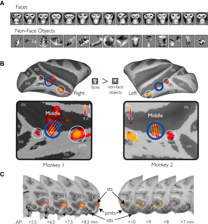
Visual stimuli consisted of images of unfamiliar faces and familiar and unfamiliar everyday objects. In all images, the backgrounds were removed with image editing software and the images were resized to a standard size. In fMRI experiments, the image backgrounds consisted of phase-scrambled noise, whereas in the physiology experiments the background was filled with white noise. Each image exemplar was normalized so that the mean luminance was equal across all images. In fMRI experiments, face-selective regions were identified using a contrast of 15 images of faces and nonface objects (see Fig. 1A). Neurophysiological experiments were conducted using these images in Subject 1, 15 faces and 15 nonface objects, and a subset of these images, 10 faces and 10 nonface objects, in Subject 2. For rank-ordered image analyses in Figure 12, only responses to a fixed subset of 10 exemplars per category were used in Subject 1 for an unbiased comparison to rank-ordered image responses in Subject 2.

Figure 1.

fMRI localization of face-selective patches. A, Conventional images of macaque faces and familiar everyday objects used to localize face-selective regions in the temporal lobe. Subsets of these images were also used in the neurophysiology experiments. B, Three fMRI-identified patches were found on the convexity of the lower bank of the STS. C, The MFP was observed consistently across both animals on the convexity of the STS (e.g., crown of the ITG). Only positive valued signal change to the faces-objects contrast is shown and only for voxels that were more significantly driven by the presentation of object images over scrambled versions of those images.

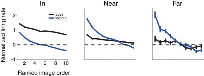
Figure 12.

Selectivity across face and object images inside and outside the pMFP. Site-by-site image responses were normalized by the site's maximum absolute response across all images and then ranked using independent data (within face or nonface image groupings; see Materials and Methods) before averaging over all sites and both monkey subjects in each of the three anatomical regions described previously (“In,” “Near,” and “far”; based on distances of 1 and 2 SDs of the fit isotropic Gaussian model). The responses to all face (black curves) and nonface objects (blue) are shown for sites in the “in,” “near,” and “far” regions. In the pMFP, the best driving face image gave a greater response than the best driving object exemplar; and outside the pMFP (middle and right panels), the response to the best driving face image was far exceeded by the response to the best driving object exemplar. To prevent any bias, images were rank-ordered on a held-out set of trials, and the remaining trials were used for plotting rank-ordered responses.

Awake functional imaging.

A plastic MRI-compatible headpost was attached to the subject's skull under aseptic surgery conditions. Upon recovery, the animal was trained using standard operant conditioning methods to fixate in a 3–4 degree window and to adopt a sphinx position while sitting in an MRI-compatible chair (Vanduffel et al., 2001). The subject was rewarded for constant fixation in the response window as 5 degree images of face and nonface distractors were presented at the center of the screen. Images were randomly jittered on each trial (±0–2 degrees in both azimuth and elevation; uniform distribution). Images were displayed for 250 ms, with an interstimulus interval of 500 ms. Eye movements were monitored with an optical eye tracking system (ISCAN). Time points where the animal broke fixation for >250 ms were excluded from further analysis. Images were shown in blocks of 3–5 stimulus categories (faces, bodies, places, objects, and scrambled faces) with 20 different exemplars in each category displayed in a random order. Analyses of the functional imaging data were conducted using the FS-FAST toolbox (http://surfer.nmr.mgh.harvard.edu/fswiki/FsFast) and custom written scripts in MATLAB (The MathWorks).

MION-enhanced functional imaging was conducted on either a 3T Siemens Tim Trio (M1) at the Athinoula-Martinos Imaging Center at Massachusetts Institute of Technology or a 3T Siemens Allegra imaging system (M2) at the Athinoula-Martinos Imaging Center at Charles Town, MA. Functional data (TR = 3.2 or 3 s, 46 or 45 slices, 1.25 mm isotropic voxels with a 10% slice gap) were collected with a custom-built, single-loop surface coil. Image presentation and water reward were controlled with experimental presentation software: either MWorks http://mworks-project.org (M1) or similar software developed in-house (M2). In brief, functional data were motion-corrected across all sessions and coregistered to the animal's anatomical reconstruction with FMRIB's FLIRT software package. Field scans were taken during each session conducted at the Massachusetts Institute of Technology imaging center and used to correct magnetic field distortions with FSL's FUGUE software package (Jenkinson et al., 2012) in M1. fMRI data from M2 have been reported previously (Op de Beeck et al., 2008; Issa and DiCarlo, 2012, Issa et al., 2013).

Multiunit electrophysiology.

At the conclusion of functional imaging experiments, the animals were prepared for neurophysiological recording by the placement of a plastic, MRI-compatible recording well (18 inch diameter; Crist Instruments) under aseptic conditions. The recording chamber was placed to target the middle face patch as localized with fMRI. M1: Right hemisphere, Horsley-Clarke center anteroposterior coordinates 3 mm, with a 9 degree electrode angle in the coronal plane, beginning at ∼19 mm mediolateral. M2: Left hemisphere, Horsley-Clarke center anteroposterior coordinates 14 mm, with an 8 degree angle beginning at ∼21 mm mediolateral. The animals were trained to sit upright in a standard neurophysiology recording chair and fixate in a 2–3 degree response window while viewing images of faces and nonface objects in a standard rapid sequence (M1: 7–10 images/trial, 200 ms on 100 ms off or M2: 12–15 images/trial, 100 ms on and 100 ms off). Each image was repeated either 12 (M1) or 3–5 (M2) times and presented in pseudorandom order. Eye movement traces were collected and monitored with an optical eye tracking system (EyeLink, SR Research). Trials where the animal broke fixation were aborted, and only images presented before an eye movement were considered. The first image in an RSVP sequence was always disregarded from further analysis.

Multiunit recording was conducted with glass coated tungsten microelectrodes (0.5–0.7 mΩ: Alpha-Omega), amplified with a BAK system (BAK Electronics). Neural signals were sampled at 14 or 8 kHz and bandpass filtered with an online Butterworth filter (Krohn-Hite) between 300 Hz and 7 kHz (M1) or 300 Hz and 4 kHz (M2), before being thresholded to determine the multiunit spike counts. Multiunit detection thresholds were determined in the recording sessions each day by the experimenter and were set to 1–2 SDs above the noise. Experimental stimulus and reward control, as well as data recording and storage, were managed by MWorks software (http://mworks-project.org) on a Mac Pro running OS 10.5–6. Straight (Crist Instruments), and custom-made angular (5 and 7 degree) grids were used in the recording chamber to lower the tip of a 26 gauge stainless steel guide tube ∼5–6 mm from the STS. Microelectrodes were lowered through the guide tube using a hydraulic microdrive (David Kopf Instruments), and while carefully listening for cell transitions, the microelectrode was advanced until the distinct sound of crossing the STS was heard. Sites were then recorded at 200–500 μm intervals in the lower bank of the STS and more laterally along the convexity of the inferior temporal gyrus (ITG). Single-unit data were obtained by sorting the multiunit data from M2 using the wave_clus software toolbox for MATLAB (Quiroga et al., 2004) and accepting units with a ≥5x signal-to-noise ratio (peak-to-peak amplitude vs SD).

fMRI analysis.

Standard univariate methods were used to analyze fMRI data as implemented in FS-FAST. The functional signal was spatially smoothed (Gaussian kernel, 2.5 mm FWHM) in the volume. We only examined visually active voxels (e.g., voxels that had a significant response to visual images over scrambled objects; p < 10e-6) to localize category-selective voxels for neurophysiology experiments. Category-selective voxels were defined as voxels that met both the visually active criteria and had a significant response to faces in a faces-objects contrast. Face-selective regions in central IT were then targeted under the guidance of a custom stereo microfocal x-ray imaging system (Cox et al., 2008). Caret software was used to visualize activations on inflated surfaces of the 2 monkeys (Van Essen et al., 2001).

Neural analysis.

The multiunit response to an image was recorded as the average spike rate in a fixed window 60–160 ms after stimulus onset. Responses to each image exemplar were baseline subtracted using the average firing rate in a window 0–50 ms after stimulus onset across all repetitions of the image exemplar. Although there may be changes in baseline over the course of a trial, the presentation of image exemplars was randomly interleaved; thus, any baseline shifts within trials were counterbalanced across images. The average response to all repetitions of a given category (regardless of the specific image exemplar) was used to estimate the mean and SD of the category-selective response (e.g., faces or nonface objects). A face preference metric for each site was defined and measured as d′ as follows:

where X̄_faces (σ_faces²) is the mean response (variance) across all presentations of face images and X̄_objects (σ_objects²) is the mean response (variance) across all presentations of nonface images (Issa and DiCarlo, 2012; Ohayon et al., 2012). Response variance can also be computed using only the average response to each image (Afraz et al., 2015). Here, we measure response variance across individual image presentations because this metric does not vary in expected value with the number of presentations of each image, an experimental variable that arbitrarily varies across studies. In this context, it is important to note that the d′ values used here, while technically most appropriate as a standard for comparison, are lower than d′ values reported in other studies (e.g., Afraz et al., 2015), which average over repetitions of each image. A final selectivity metric that is commonly used is to compute a face selectivity index (FSI) from the mean responses to faces and nonface objects. To allow direct comparisons to previous reports of face-preferring neurons, we calculated FSI as a second face preference metric (Tsao et al., 2006; Freiwald et al., 2009; Bell et al., 2011) as follows:

Following the conventions of previous studies, we defined FSI at sites as follows: (1) when X_faces < 0 and X_objects > 0, then FSI = −1 (n = 113 sites; 11%); (2) when X_faces > 0 and X_objects < 0, then FSI = 1 (n = 244 sites; 25%); and (3) when X_faces < 0 and X_objects < 0, then FSI = −FSI (i.e., if the sites were inhibited by the presentation of images of faces to a greater extent than to images of nonface objects, then these sites were also considered to be “face-preferring”; n = 117 sites; 12%).

To determine how reliable the face selectivity metric was at each site, we computed the split-half reliability across repeated presentations of the images. Repeated presentations of each image were randomly assigned to two equal pools, and the faces versus objects selectivity measure was calculated for each pool. The random splitting procedure was repeated (n = 1000) for each site. The average correlation between the two sets of measures, across all sites, was corrected for the use of only half the trials in generating the estimate (Spearman, 1910) and taken to be the reliability of the face selectivity measure at each site.

To characterize the variability in category selectivity at nearby, but different spatial positions in IT, we computed the squared difference of selectivity from pairs of sites sampled on the same penetration and within close spatial proximity to each other (<500 μm based on microdrive readings, which have 1 μm resolution, no x-ray measurements used). We averaged the values computed over all such sites and termed this var1. To ask whether this spatial variation was greater than that expected by chance, we compared this to the variability expected from: (var2) “noise” (variability over repeated image presentations) and (var3) variability expected by different choices of specific face and nonface images.

var2.

To estimate the expected variability due to just repetition “noise,” all measured responses at each site were randomly split into two equal halves, where each half contained the responses to all face and nonface images. The squared difference in face selectivity (d′) determined from each split was computed for each site and then averaged across all sites (var2). The variance here reflects only the lack of perfect repeatability to the nominally same stimulus conditions. To eliminate any impact of the random choice of group split, n = 1000 random splits were done, and we report the average var2 value over all such splits.

var3.

To estimate the variability in the measured face selectivity at each site that might result from the fact that we tested only a finite number of images, we followed a similar procedure as above, splitting the data at each site into two groups. But in this case, the split was by images: half of the face and object images used in the experiment were included in one group, and the other half of the images were included in the other group. Because this procedure also includes the former variability source (“noise” in repeated presentations of the same image), var3 is expected to be larger in magnitude than var2. To ensure that all three measures of variability (var1, var2, and var3 above) could be directly compared, we ensured that equal numbers of samples were used to estimate category selectivity. In some cases, this meant subsampling from one source of variability. For example, the same number of images and repetitions went into the estimates of category selectivity for estimating the variance due to image repetitions as went into estimating the variance within penetration as a function of the distance between sites.

Measurements of purity were estimated by counting the proportion of sites that met a “face-selective” threshold criterion (see Results) on the face preference metric (either d′ or FSI, above) as a function of the 2D spatial distance from the center of the MFP. Multiunit sites were binned into nonoverlapping bins with equal counts (M1 = 28 sites/bin; M2 = 31 sites/bin), and the proportion of face-preferring sites in the bin was taken as the estimate of the purity. The location of the bin was the average radial distance of the sites allocated to the bin. The resulting purity function was smoothed over 5 bins for presentation in Figure 8. As the exact position of the center was dependent on the specific spatial model, we estimated the purity relative to the centers computed for each of those models. In Figure 9, we used equal, sliding 1 mm bins (5 site minimum) to perform a direct comparison of single-unit data (SUA) and multiunit data (MUA) purity as a function of spatial distance.

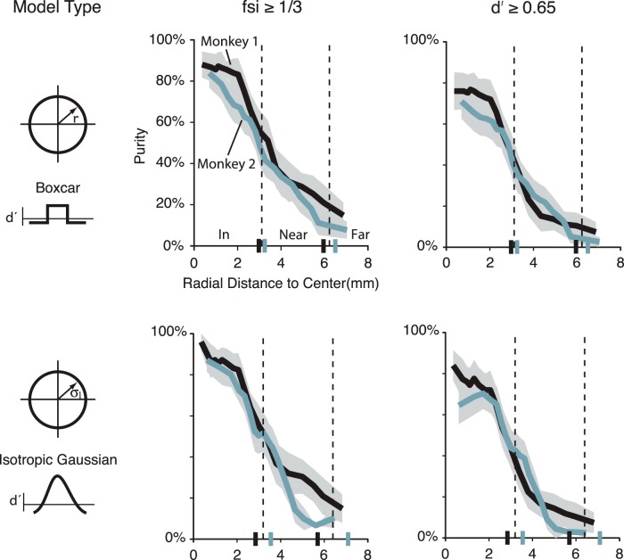
Figure 8.

Functional selectivity and purity estimates in the pMFP as a function of spatial size. Estimates of the fraction of category-selective multiunit sites in the MFP (the purity) could range from 94% to 58% depending on the distance from the center of the patch. These ranges varied due to both the model and metric used to define the patch. Purity estimates based on an FSI > 0.33 led to higher overall purity estimates than those based on a comparable d′. Overall, the purity falls off gradually from the center of the patch to cortical regions outside the patch. Dotted lines indicate the radial average distance from the center, which defines the qualitative distance categories: “in,” “near,” and “far,” where “in” is defined as less than radius value determined in the model fit and “far” is > 2 times the radius value. Small vertical lines on the abscissa indicate 1 and 2 times the radius value for each subject by model type.

Figure 9.

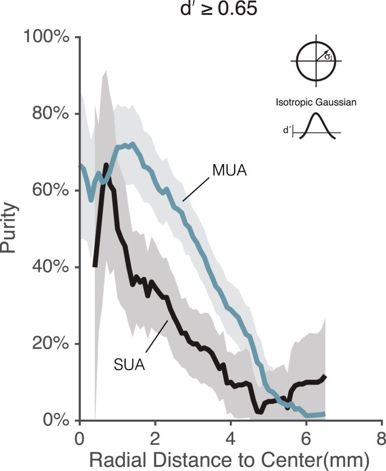
Comparison between single-unit and multiunit purity estimates in the pMFP as a function of spatial size. Spike waveforms from Subject M2 were sorted to provide SUA. Using the center of the isotropic Gaussian model fit to the MUA data, we plotted the fraction of face-selective sites (purity) for both MUA (gray line) and SUA (black line) as a function of distance from the center. In both cases, a site was defined as face-selective if its d′ was ≥0.65. Both MUA and SUA produced a gradual fall-off in purity over a similar spatial range, although MUA data showed slightly higher d′ values and thus slightly higher purity estimates. Gray line indicates Monkey 2 curve in Fig. 8, but using sliding 1-mm-wide spatial bins to exactly match the procedure applied to the SUA. Error bands indicate the SEM of the estimated purity values determined by bootstrap (see Materials and Methods).

We examined the distributional form of the face preference metric (d′) estimated from multiunit sites located in each of the three regions (“in,” “near,” and “far”) around the MFP (defined by the model analysis). Each sample was fit to a generalized extreme value (GEV) function. The GEV function is a distribution that combines the Gumbel, Frechet and Weibull distribution into the same generalized formula. The function has the following form:

Intuitively, the GEV function is primarily used to model a distribution consisting of extreme values. For example, if one were to measure face selectivity for all of the cells in IT, it would be reasonable to assume that this distribution would be normally distributed and that the face selectivity measured for cells in the MFP would have very high selectivity for faces compared with the selectivity measured at sites outside the face patch. These MFP face-selective measurements would be extreme valued relative to the distribution (i.e., significantly different from the distribution of values obtained from sites outside the face patch). Modeling these types of distributions is typically done by extreme value functions in the fields of engineering and mathematics and was used here to provide distributional fits to our data. The face preference metric at each site was collapsed across M1 and M2 according to the isotropic-Gaussian model. We assessed the goodness of fit for our data to the GEV distribution using a two-sample Kolmogorov–Smirnov test. The parameter values for the GEV distribution were used to characterize the form of the face selectivity distributions.

Ranked image analysis by spatial zones.

We examined the rank-ordered response to individual faces and object exemplars at each site, averaged over the “in,” “near,” and “far” spatial zones that we defined for the physiologically defined MFP (pMFP). This analysis was conducted by using a subset of image presentation repetitions (2/3) at each site to determine its rank order (i.e., most preferred to least preferred) over the 10 face images and its rank order over the 10 object images. The data from the remaining repetitions (1/3) were used to estimate that site's response to each of the images. This procedure avoids biasing the rank plot's slope due to variation (noise) in the responses. The estimated responses to all of the images were then normalized by the greatest absolute response across all 20 images. This produces two ranked response plots for each site (one for faces and one for objects). These two ranked response plots were than averaged across all sites in each spatial zone (in, near, or far) to create the population rank-ordered response in each spatial zone.

Cortical surface models.

Anatomical models of the white and pial surfaces were estimated from averages of multiple (6–8) high-resolution anatomical MRI volumes (500 μm isotropic T1-weighted anatomical volumes) taken under anesthesia in an MRI-compatible stereotaxic frame (Crist Instruments). The mid-layer surface model used in our analysis was estimated by taking the midpoint between the estimated white and pial surfaces. The area of the surface to flatten was chosen arbitrarily by centering a point in the fMRI identified MFP and finding a closed boundary of mesh nodes that were a specified distance (radius = 7 mm) from the center. The radius was chosen so that it maximized the cortical surface for the analysis but did not include face-selective activations from anterior, medial, or posterior patches additionally present in IT. Our goal was to characterize the spatial structure in face-selective signal attributed to the MFP, so we sought to minimize spatial interaction with other face-selective regions. High-resolution (i.e., small internode distance) patches were created by upsampling the closed mesh using custom scripts and toolboxes in MATLAB (Wavelet meshes toolbox) (Peyre, 2009). Finally, the manifold was computationally flattened to preserve geometry using the MRtools MATLAB toolbox (Heeger Lab: http://www.cns.nyu.edu/heegerlab/wiki/doku.php?id=mrtools:top).

x-ray localization and registration.

The electrode position for every site sampled was estimated in 3D space using a custom-built stereo microfocal x-ray system (Cox et al., 2008). Briefly, the x-ray system uses two x-ray sources (Oxford Instruments) and digital image capturers (Shad-O-Snap, 1024; Teledyne/Rad-icon Imaging) positioned around the monkey's head in the recording setup. Six brass fiducials (diameter ∼500 μm) were positioned in known locations on a rigid frame attached to the animal's skull. The x-ray system produced images in two known planes that contained both the fiducials in the frame and the electrode tip. Custom software was used to reconstruct the 3D location of the electrode tip, based on the known locations of the fiducials and the inferred geometry of the x-ray sources and detectors. Wells drilled into the fiducial frame at known positions were filled with CuSO₄, and an MRI anatomical volume was used to register the electrode positions to the high-resolution anatomical volume using FMRIBs FLIRT and FNIRT registration tools (Jenkinson et al., 2012).

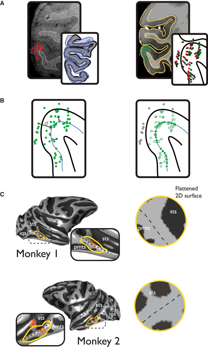
The recorded sites were colocalized to the 3D anatomical volume of each subject. This registration was performed in two steps, a linear affine registration between the 3D anatomical volume and the reference volume coregistered to the x-ray frame (see Fig. 2A, left inset) followed by a nonlinear registration using FMRIB's FNIRT tool. The nonlinear registration process was used to adjust for distortion in the shape between the reference volume used for coregistration with the x-ray system and the computational anatomical model used in the functional imaging studies. These adjustments were applied to the 3D positions of the sampled sites (see Fig. 2A, right, inset), generally resulting in small changes in spatial position relative to the linear registration. Each recording site was then projected to the closest orthogonal node on a surface manifold created from each subject's anatomical volume. We discarded any recorded sites that moved >1250 μm from the original 3D location to the projection site on the mid-layer surface model (∼14% Monkey 1; ∼25% Monkey 2; 53% for putative single units sorted for Monkey 2). Spatial analyses were conducted on high-resolution flattened 2D surfaces of the area around the fMRI-identified MFP. The location of each recording site on the 2D surface was recovered from the position of its corresponding surface node after flattening.

Figure 2.

Spatial registration and analysis methods. The 3D spatial locations of all sampled sites in the MFP region were estimated with a custom-built stereoscopic x-ray imaging system. The 3D locations were registered (A, left) to a high-resolution (500 μm) anatomical MRI. Anatomical variability before (gray cortical ribbon; left, inset) and after neurophysiological recordings (blue cortical ribbon, left inset) can result in subpixel registration error. To improve the overall accuracy of the registration, nonlinear registration using FMRIB's FNIRT registration tool was performed (A, right), and the resulting transform was applied to the estimated positions of the recording sites (A, inset represents the overall spatial movement of sites projected in a 2D slice). The spatial position of each recording site was projected to the closest orthogonal node of a high-resolution mid-layer mesh of the cortical surface (B, left). Sites that moved a distance >1250 μm from their original 3D position to the 2D surface manifold were excluded (B, right, gray dots) from further analysis. The area for analysis was selected by choosing the approximate center of the fMRI MFP activation in each monkey and including all nodes on the cortical mesh within a maximal geodesic radius (7 mm). The radius was chosen to be approximately the greatest distance that would not encroach into face-selective activations at posterior (PL) or anterior (AL) locations.

Fitting models of the spatial distribution of face-preferring IT sites.

We fit a Gaussian and a simple hard-walled circle (boxcar) model by least squares to the 2D spatial profile of face selectivity across recording sites. Evaluation of the models was conducted with custom-written code in MATLAB and modified toolboxes (Mineault, 2011). In brief, each model predicts a selectivity value for each site given its spatial 2D location. The Gaussian and boxcar model are defined by a 2D center position (x₀ and y₀) and a measurement of dispersion (i.e., the SD of the Gaussian or the radius of the boxcar). The latter parameters were taken as the estimate of the radius of the (neurophysiologically determined) MFP under each model. The model parameters and linear weights were estimated by a coarse to fine brute force search of the parameter space, minimizing the error between the estimated selectivity and the observed selectivity of the data. The domain of the spatial parameters was limited by the size of the cortex defined by the flattening procedure (e.g., the radius or center position could not extend to a position outside the flattened mesh; for the relative size of the model to the size of the flattened mesh, see Fig. 5). The SEs of the parameter values were estimated by bootstrap methods.

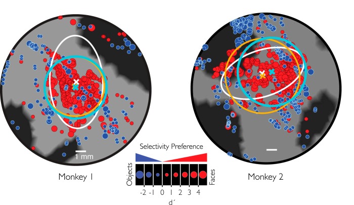
Figure 5.

Low-frequency 2D spatial models of the pMFP are largely consistent. The spatial location and category preference for each recording site are localized on 2D flattened surfaces of the fMRI-identified MFP region. The different best fit models from our analysis are largely consistent in their estimate of the center and the spatial extent of the enriched region. Scale bars represent 1 mm.

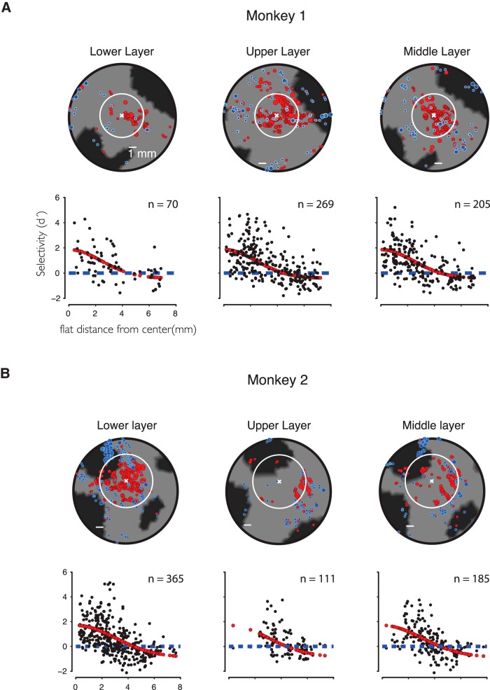
To examine the 3D layer information in our data, we created 3D models of the upper and lower layers of the cortical ribbon. These models were generated following the same procedures described previously for creating our standard 3D models of cortex. The model of the upper portion of the cortical ribbon was created so that it would extend from the outer pial surface to a depth of ∼500 μm below the pial surface. Similarly a model of the “lower” portion of the cortical ribbon was created to extend from the white matter border (or the putative bottom of the cortical ribbon) to a depth of ∼500 μm above the white matter border. To uncover any possible differences between the upper and lower layer sites in our data, we limited our analysis to sites that moved <500 μm from their original 3D position to their projected location on either of these upper or lower layer models (M1: n_upper = 269, n_lower = 70; M2: n_upper = 111, n_lower = 365). This ensured that sites located in the upper layer were not also analyzed in the pool of sites located in the lower layer.

Results

Our goal was to neurophysiologically map and characterize the cortical tissue in and around the fMRI-defined MFP with respect to face selectivity. To functionally localize the MFP in the ventral temporal lobe, we first tested face versus nonface object selectivity using fMRI in two awake, behaving macaque subjects using MION contrast agent (Fig. 1). Conventionally posed and cropped images of unfamiliar conspecific faces and familiar everyday nonface objects were used in both the fMRI and neurophysiology experiments. fMRI maps for all object driven voxels (unthresholded; see Materials and Methods) are shown in Figure 1 for the faces versus nonface objects contrast. In both monkeys, these maps demonstrated three large clusters of voxels along the posterior, middle, and anterior convexity of the STS. Because these results are consistent with previous work (Tsao et al., 2003, 2008), we follow the naming conventions introduced in that work. The “posterior face patch” was located near the inferior occipital sulcus on the gyrus between the posterior middle temporal sulcus and the STS in area posterior inferior temporal cortex. The MFP extended across the lip of the STS, localized near the end of the posterior middle temporal sulcus in central inferior temporal cortex. Finally, the “anterior face patch” was localized to the gyrus between the STS and the anterior medial temporal sulcus in anterior inferior temporal cortex (anterior inferior temporal cortex, central inferior temporal cortex, and posterior inferior temporal cortex are subdivisions of IT based on Felleman and Van Essen, 1991). We also observed a number of other clusters in IT cortex possibly corresponding to MF (middle fundus in the STS), AF (anterior fundus in the STS), or AM (anterior medial IT) as reported in previous fMRI work (Tsao et al., 2008). The MFP was approximately similar in spatial extent under fMRI across the two animals. We observed the most posterior extent of the fMRI activation at AP 5.5 mm in Monkey 1 and AP 7 mm in Monkey 2. In both animals, the fMRI activation extended across ∼5 mm and predominately covered the crown of the ITG.

Neurophysiological experiments were conducted with standard single microelectrode recording methods. We targeted recording sites in and around the location of the MFP using a custom-designed stereo microfocal x-ray imaging system (see Materials and Methods). This system allowed us to reconstruct the 3D position of the recording electrode tip at each site sampled in IT cortex with submillimeter tissue-based accuracy. We then projected the positions of all the sampled sites to a 3D cortical surface model of each subject's brain, which were derived from T1-weighted structural scans. A summary of the steps involved in the registration of the sampled sites to the cortical anatomy is shown in Figure 2 (see Materials and Methods). The spatial extent of the region where sites were sampled was chosen to maximize anatomical coverage without extending so far as to encroach upon the anterior or posterior face patch regions observed with fMRI, which are in subdivisions of IT (posterior inferior temporal cortex and anterior inferior temporal cortex) separate from central inferior temporal cortex. We also sought to avoid the distinct activation that lay medial in the STS, likely corresponding to the fundus patch reported in previous work (Tsao et al., 2003). Under these constraints, a 14-mm-diameter region centered on the MFP in each monkey was chosen for inclusion in this study (Fig. 2C).

The face preference of each recorded site was measured as d′ for faces versus nonface objects using a subset of the images used to identify face-selective patches in the fMRI experiments (see Materials and Methods). All sites were projected from their original 3D x-ray estimated position to a midlayer representation (e.g., 2D surface manifold in 3D space) of the cortical surface for each monkey under the assumption that face selectivity varies transversely along the cortical mantle (this 2D assumption was checked by supplementary 3D analyses; see Discussion; see Figs. 13, 14). The surface was then computationally flattened (from its native 3D space to a near-isometric 2D space) before analyses (see Materials and Methods).

Figure 13.

Upper and lower regions of the cortical ribbon show similar selectivity profiles. Dividing sites that could be reliably (see Materials and Methods) localized in the “upper” or “lower” layers did not reveal additional spatial structure. For comparison, sites localized to within 1 mm of the middle of the cortical ribbon were used to create a “middle layer.” These sites could overlap upper and lower layer sites. A, Monkey 1. B, Monkey 2. Scale bars represent 1 mm.

Figure 14.

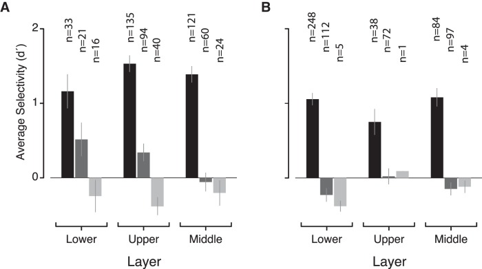
Face selectivity estimates for upper, lower, and middle cortical layers. Separating sites by upper and lower layers produces similar selectivity estimates of the average selectivity in the “in,” “near,” and “far” regions (black, dark gray, and light gray bars, respectively), in either subject (A: Monkey 1; B: Monkey 2).

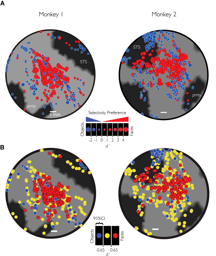
As shown in Figure 3, we found a zone enriched with sites that each demonstrated a response preference for images of faces over nonface objects. This enriched zone was located along the ITG in area central inferior temporal cortex, corresponding to the MFP region localized with fMRI. A similar zone was found in each of the 2 monkeys. Hereafter, we refer to this physiologically measured region of enriched face-preferring sites as the pMFP. In this study, we focus exclusively on characterizing the spatial structure of the pMFP and do not consider its relationship to the fMRI-defined MFP any further (for those comparisons, see Issa et al., 2013).

Figure 3.

pMFP contains an enrichment of face-preferring sites. A, Flattened 2D regions of the temporal lobe highlight category preference. Red represents sites that prefer faces over objects. Blue represents sites that prefer objects over faces. M1, n = 425; M2, n = 565 multiunit sites. The size of each circle represents the strength of selectivity at each site. B, Distribution of highly category-selective sites. Red or blue sites responded preferentially to faces (d′ > 0.65) or objects (d′ < 0.65), respectively. Yellow represents sites where the 95% CI of the site's selectivity metric fell within [−0.65, 0.65] and thus is not significantly above (or below) those two thresholds. Scale bars represent 1 mm.

While there was a clear enrichment for face-preferring sites in the pMFP, it was also evident that there was variation in face selectivity throughout the region. Some sites displayed a stronger preference for faces than other nearby sites (Fig. 3, different sized red circles), and some sites showed face preference that was the inverse of that predicted; they clearly preferred images of nonface objects over images of faces (Fig. 3, large blue circles). This variation in the face preference metric (d′) was not due to physiological noise (e.g., Poisson spiking variability) as our selectivity estimates were reliable across different trial subsamples of the data (the split-half correlation, or reliability, for Monkey 1 was r = 0.98, and r = 0.92 for Monkey 2).

In previous work, sites were considered face “selective” if the response to images of standard faces (averaged over all face images) was at least twice as large as the response to nonface objects (averaged over all nonface object images). Using similar criteria (see Fig. 7 for the estimate of this value), we also found variation in the spatial organization of face selectivity, where nonface object selective sites were near face-selective clusters (Fig. 3B). In summary, the pMFP in each monkey appeared to consist of a single region without large intervening subregions. We also observed significant site-to-site variability in face preference.

Figure 7.

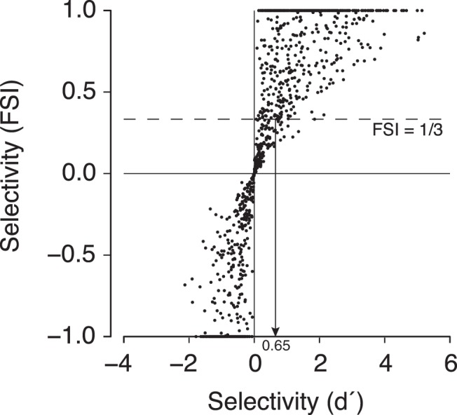
Direct comparison of d′ and FSI contrast metrics. Absolute values of d′ depend critically on how one defines response variance (see Materials and Methods). The FSI metric displays an approximately linear relationship to selectivity measured with d′. In our data, an FSI ∼ 1/3 is equivalent to a range of d′ values with a median of 0.65. Most of these sites with a d′ > 0.65 have a face image preference significantly different from zero (422 of 424 sites with d′ > 0.65 had a bootstrapped 95% CI >0).

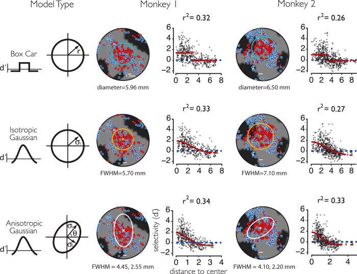
To quantitatively characterize the spatial profile of the pMFP, we fit three different spatial models to the 2D data. These models were based on the observation that the pMFP appeared as approximately a single subregion (Fig. 3) and upon ideas implicit in the fMRI literature: (1) a simple in-versus-out module or boxcar model, (2) a circular (isotropic) Gaussian model, and (3) a three parameter Gaussian model that allowed for a nonisotropic, or an elliptical shape (Fig. 4). All three models were parameterized by a center position (x and y) and a measure of spatial spread. The boxcar model was parametrized by a radius parameter (i.e., in vs out), whereas the isotropic Gaussian model was parameterized by its spatial dispersion (i.e., its SD). The nonisotropic Gaussian model had two parameters of dispersion (reflecting the major and minor axis of the elliptical shape) and an angle parameter to allow rotation on the 2D cortical surface. The model parameters were fit to the data by linear regression: the linear coefficients acted as scale factors to describe the peak selectivity in and out of the patch. In Monkey 1, all three models resulted in an approximately similar fit quality to the data (r² ∼ 0.3), whereas Monkey 2 demonstrated a small but significantly better fit with the higher parameter model (r² = 0.33 vs 0.26, nonoverlapping 95% CIs estimated by bootstrap). In each monkey, the absolute center of each model was relatively consistent across models (Fig. 5), and each model made very similar predictions on the size of the enriched zone of face selectivity (6–7 mm diameter). The radius parameter of Model I was taken to be the estimated size of the patch under a module type hypothesis (e.g., the diameter of the MFP in the 2D flattened space was twice the size of the estimated radius), whereas the FWHM of the Gaussians in Models II and III were taken as an estimate for the size of the patch. It is notable that, whereas the millimeter-scale spatial profile of the pMFP was qualitatively well captured by all models (Fig. 3), the overall fits were low in general in that they each explained only approximately one-third of the variance. For example, examination of the 1D collapsed model plots (Fig. 4) shows that there are often large deviations between the actual face selectivity in the data at a given spatial position and the face selectivity predicted from the model. This suggests that none of the models examined would be able to capture the detailed spatial structure of the pMFP, consistent with prior work showing reliable high spatial frequency information for category selectivity in IT (Issa et al., 2013) (see Discussion).

Figure 4.

2D models of the spatial organization of face selectivity on the pMFP. Three models (rows: box car, isotropic Gaussian, and anisotropic Gaussian) for the spatial structure of the pMFP were used to fit the category selectivity and 2D spatial position over all multiunit samples. Column 1 summarizes each model and their 2D spatial parameters parameters (see Materials and Methods). Column 2 (monkey 1) and column 3 (monkey 2) summarize the results in each subject. The best fit models are displayed as outlines on the flattened 2D cortical maps (left) with the estimated size parameter for each model type underneath. In addition, the collapsed, 1D selectivity profiles (right) as a function of radial distance are shown (black dots represent individual sites), and the collapsed model prediction is overlaid in red. Abscissa units are in millimeters for the box car and isotropic Gaussian models (rows 1–2) and in number of SDs for the anisotropic Gaussian model (row 3) since the isocontours for this model were not radially symmetric. Variance explained was calculated as the correlation of the model predictions (red) with the individual site d' values (black dots) at the corresponding location (values were not corrected for noise in the neural data, but see Fig. 6 for estimates of noise levels). Scale bars represent 1 mm.

The analyses in Figure 3 show that sites neighboring each other in the MFP can differ significantly in their measured preference for images of faces versus images of nonface objects. To determine how much of that variation was due to true differences in the selectivity of nearby sites, we sought to carefully eliminate any extra measurement variation caused by our techniques. First, because those analyses were conducted on a flattened 2D representation of the cortical mantle, some of the apparent variability in face selectivity may result from the small shifts in spatial position induced by projecting sites from 3D space to the 2D sheet. To remove this possibility, we characterized the variance in face selectivity (Δd′) between pairs of nearby sites recorded on the same electrode penetration in native 3D space at small spatial scales (i.e., sites collected within 500 μm of each other on the same penetration in the same recording session; see Materials and Methods). This analysis is more spatially precise because it avoids 3D to 2D projection errors. In addition, by restricting analyses to sites recorded on the same electrode penetration, we could rely on the highly accurate readings of our microdrive (∼1 μm resolution) for estimating the separation between sites. With this analysis, we still found large differences in face selectivity in local pairs of sites (<500 μm separation; average absolute Δd′ was 1.04 for Monkey 1 and 0.75 for Monkey 2, respectively; see Fig. 6). So we then asked: is this true variation in the underlying face selectivity of nearby IT sites, or might it be induced in our measurements by “noise” (i.e., spike count variability in response to the identical image) or by the particular choice of images we tested? To do this, we quantified the expected amount of variability in measured face selectivity (by carefully resampling our own data, see Materials and Methods). This showed that both the expected “noise” variance and expected image sampling variance are far too small to account for the observed variance in face selectivity of nearby IT sites. In sum, our analyses converge to show that the variability in face preferences between sites within the MFP is due to true underlying neural differences in face selectivity. This lack of uniformity argues against simple modular models (see Discussion).

Figure 6.

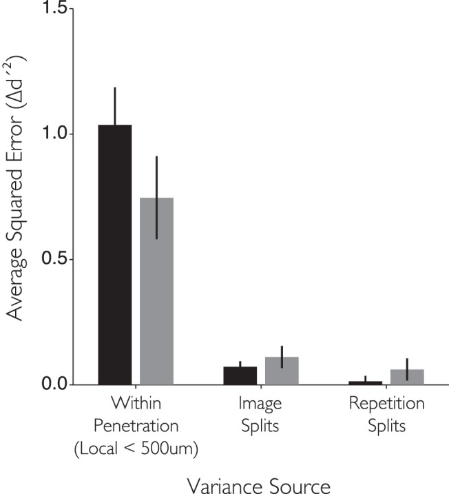
Variance in selectivity estimated at nearby spatial locations in the MFP. Bar graph represents the average squared difference in face selectivity between sites recorded on the same electrode and <500 μm apart from each other. The average difference between sites expected simply from the use of a limited number of image exemplars or trials is also depicted for comparison. Error bars indicate the 95% CI on the estimate. Black and gray bars represent Subjects 1 and 2, respectively.

Previous studies estimating the proportion of face-preferring sites in the MFP, referred to here as “purity,” have reported that the fraction of face-selective units in the MFP was either ultra high (97% in Tsao et al., 2006) or very high (84% Freiwald et al., 2009, 2010; Ohayon et al., 2012), whereas other studies that have sampled the margins of the face patch reported a more modest purity estimate (<50%; Bell et al., 2011). The modest purity rates reported by Bell et al. (2011) could suggest spatial structure (i.e., nonuniform selectivity) in the MFP. To explore the possible spatial structure of purity in the MFP, we used the high spatial resolution of our methods to measure the purity of the MFP as a function of distance from the center of the patch (see Fig. 8). In doing this analysis, we used images and selectivity metrics similar to previous reports, but also used other well-behaved metrics (d′) with the goal of giving a more complete characterization of the MFP (Fig. 7). Because all three of the spatial models we tested produced similar fits to our data, we limited our analysis to the two simplest models: the isotropic Gaussian model and the module or boxcar model. We first defined a neuronal site as face “selective” if it had a face preference index (d′, faces vs objects) > 0.65. We also used a contrast metric (FSI) similar to what has been used in previous studies to estimate face selectivity (Tsao et al., 2006; Freiwald et al., 2009, 2010). The FSI ranges from −1 to 1, and sites that had an FSI >0.33 (response to faces at least twice as strong as response to nonface objects) were considered to be face-selective. We chose a d′ = 0.65 cutoff because it is the median d′ of neurons with FSI near 0.33 (Figure 7, gray region). An additional analysis also confirmed that the vast majority of sites in our data with a d′ >0.65 had selectivity significantly >0 (422 of 424 sites had 95% CI > 0 where CI was estimated by bootstrap resampling). The analyses demonstrated that the purity of the MFP could range from near 96% at its center (M1, FSI metric, and Gaussian model) to <50% for much of its outskirts (i.e., > 3–3.5 mm from its center) but remained at 4%–8% for tissue well outside the MFP.

Not surprisingly, the exact absolute levels of reported purity both in and out of the MFP depended on the exact spatial model and type of face selectivity metric used. However, the spatial profile of the estimated purity displayed a graded fall-off for all metrics and models tested. To quantify how the purity changed over distance relative to the size of the patch, we used the boxcar model to define three distinct spatial zones: “in” (<1 radius from the estimated pMFP center, “far” (region greater than twice the radius from the estimated pMFP center), and “near” (the intervening annular spatial region). Using the boxcar model, the d′-defined purity of the MFP “in” region as a whole averaged 67% across both subjects (d′ purity: M1 = 74%; M2 = 60%; FSI purity: 76%, M1 = 84%, M2 = 68%). The d′-defined purity of the “near” region averaged 16.5% across both subjects (d′ purity: M1 = 16%, M2 = 17%; FSI purity: 28%, M1 = 32%, M2 = 24%), and the d′-defined purity “far” from the MFP averaged 6% (d′ purity: M1 = 8%, M2 = 4%; FSI purity: 12.5%, M1 = 14%, M2 = 11%). Thus, depending on how accurately and frequently the center of the pMFP had been targeted in previous studies, purity estimates could vary dramatically. Furthermore, we were able to sort putative single units from our multiunit data (n = 288) in one subject (M2). As observed in previous studies (Issa and DiCarlo, 2012), we found a strong correlation in the face selectivity (d′) measured between the MUA and SUA (r = 0.78, p < 0.01). Performing the same spatial analysis on the putative single unit data produced a gradual fall-off in SUA measured purity with distance from the center of the pMFP, and this fall-off to baseline purity levels covered a similar spatial range as the MUA purity fall-off; however, SUA had lower d′ values than MUA, resulting in lower overall purity at any given spatial distance (see Fig. 9).

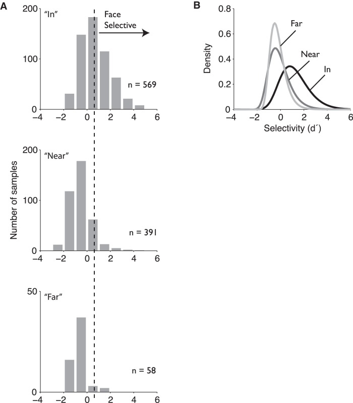
A strong form of the modular hypothesis is that face selectivity is uniformly high across the MFP, but our results (Figs. 8–10) clearly reject that hypothesis. This implies that the IT tissue in and around the MFP may not have any special anatomical boundaries or unique processing mechanisms. We next looked for alternative evidence that might support that idea: we asked whether the distribution of face selectivity for sites inside the pMFP is of a different distributional form than for sites outside the pMFP (e.g., perhaps arising from selectivity-generating mechanisms unique to the MFP tissue). Alternatively, the null hypothesis is that the distribution of face selectivity is the same both inside and outside the pMFP, only differing in their first moment (mean). To examine this issue, we analyzed the face selectivity (d′) distribution in the three regions defined previously: “in,” “near,” and “far” (Fig. 11). The empirical distributions of the face selectivity metric for the neural populations in and around the MFP demonstrate three findings. First, the average face preference index of the population of neuronal sites “in” the MFP is approximately two times higher than the population of sites “far” from the MFP (Fig. 11), consistent with the analyses above (Fig. 4). Second, we found that the selectivity distributions from all three spatial areas were significantly non-normal (Kolmogorov–Smirnov test = [0.41, 0.13, 0.29], in, near, and far, respectively, all p < 0.001). To compare the face selectivity distributions in each spatial region, we fit each distribution to a GEV function. As expected, the mean d′ values of the “in” and “far” distributional fits were different (μ_In = 0.69, μ_Near = −0.48, μ_Far = −0.52). The estimated SD of the distributional fits also differed between the three spatial regions (σ_In = 1.08, σ_Near = 0.78, σ_Far = 0.54, d′ units). The GEV distribution has a third parameter (k) that controls the form of the distribution, this parameter was small over the three distributions (k_In = −0.10, k_Near = −0.03, k_Far = 0.03). Finally, we found that the sites with the highest degree of face selectivity were only found in the pMFP. For example, we found that ∼24% of sites “in” the pMFP (or approximately one-fourth of the sites) had strong face selectivity (d′ > 2). In contrast, we found no such sites in the “far” spatial region. Based on the distributional fits, we would predict that <0.6% (i.e., ∼6 of every 1000 sites) sites in the “far” region would have equally high face selectivity. In other words, sites with a face selectivity metric of d′ > 2 are almost 40 times more likely in the MFP than out. In summary, we observed the expected shift in the mean, in addition to a broader distribution for face selectivity at multiunit sites in the most central portion of the pMFP. Interestingly, those distribution fits allow us to now estimate that the tissue near the center of the pMFP (i.e., “in”) has a nearly 40-fold enrichment in sites that exhibit a high degree of face selectivity (d′ > 2) relative to the tissue just a few millimeters away from the pMFP (i.e., “far”).

Figure 10.

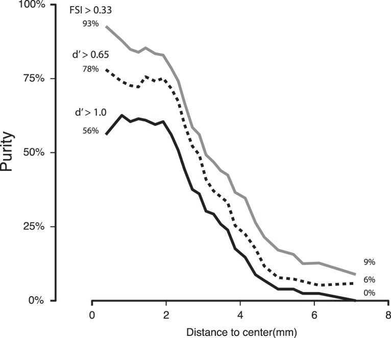
Average spatial profile of the number of face-selective sites in the pMFP. We estimated the purity collapsed across both animals using the estimated center from the isotropic Gaussian spatial model. The empirical purity function across both animals is remarkably consistent in shape across different selectivity estimators. The plot represents the proportion of face-selective sites across both animals under various criteria for face selectivity. Not surprisingly, weaker thresholds resulted in higher estimates of the purity near the center and far outside the pMFP.

Figure 11.

Distributions of face selectivity inside and outside of the pMFP. A, Distributions of the estimated face selectivity from multiunit samples in and out of the pMFP have similar distributional forms but are mean shifted and differ in their variability. B, Units outside the pMFP (light gray) appear to occupy a relatively narrow range of category-selective values (at least for this image set), with the majority of values near zero, whereas sites in the pMFP (black) are characterized by a broad range of selectivity and extreme positive values.

To examine the issue of how tuning across images within face and nonface object groupings varies as one moves away from the center of the pMFP, we plotted the rank-ordered image responses in each grouping for the same three anatomical regions defined above: “in,” “near,” and “far.” To do this, we used independent response data from each neuron to rank the image within each grouping (e.g., most preferred face to least preferred face), normalized responses from the remaining data site by site using each site's maximum absolute response across all images in the analysis, and then averaged those rank plots across all sites in each anatomical region (Fig. 12; see Materials and Methods). One possibility is that the decrease in the mean category selectivity preference for faces as a function of spatial distance from the center of the pMFP (e.g., Fig. 8) is the result of sites becoming more sparse in their image preferences while still maintaining a high response for a small set of face images. However, the data show no evidence for this hypothesis. Instead, for sites further away from the pMFP center (Fig. 12, “near,” “far”), we observed a decrease in the response to all tested face images. In contrast, we do observe a clear increase in the response to the best nonface image, but little to no increase in the response to the worst nonface image (compare Fig. 12 “near” and “far”). This latter observation is consistent with the notion that nonface object shapes are physically much more heterogeneous than face objects (Fig. 1A).

To simplify the geometric analysis involved in characterizing the spatial structure of the MFP, we modeled the cortical tissue as a flat 2D sheet and collapsed across the depth dimension. Neurons in the MFP, however, reside in the 3D volume of the cortical tissue. We thus further explored the issue of laminar differences in our data by comparing the distribution of face selectivity across different subdivisions of the cortical mantle in the MFP region (Fig. 13). Although we found no evidence for differences between lower and upper segments of the cortical ribbon, the depth errors of our x-ray system (in accurately localizing the tip of the electrode; see Cox et al., 2008) and the tissue deformation under electrode forces (Issa et al., 2010) limit our ability to generate perfectly reliable estimates of the cortical layer. Furthermore, sites sampled in the upper and lower layers were not sampled equally in the two animals. Subject 1 was mostly sampled from the upper layers, whereas Subject 2 was mostly sampled from the lower layers (Fig. 13). Despite the spatial sampling bias between the two animals, the distribution of category selectivity was similar across subjects. Separating recorded sites into nonoverlapping samples localized to either the upper or lower 1 mm sections of the cortical thickness revealed no apparent differences in the spatial organization of face preferences from the above analyses (Fig. 14). The average face preference strength of sites localized to either the upper or lower sample was greater in the MFP than in regions near or far, as defined previously. This observation suggests that there is little difference in the laminar spatial organization of face-preferring sites in the MFP between the upper and lower layers in our dataset.

Discussion

In this study, we neurophysiologically characterized the cortical tissue in and around the fMRI-defined MFP in 2 animals. Consistent with previous work (Tsao et al., 2006; Bell et al., 2011), we confirmed that the cortical tissue colocalized to the fMRI-defined MFP contains an enrichment of neural sites that prefer images of faces to images of nonface objects. Unlike previous work, our methods allowed us to provide a much more detailed understanding of the spatial organization of neural sites in and around the MFP. First, we were able to estimate that the enriched category-selective patch has a total extent of 6–7 mm on the cortical surface and determined the exact diameter depending on the definitional cutoff for face selectivity. We found no evidence that an anisotropic Gaussian model explained the data any better than an isotropic Gaussian model. Although the anistropic Gaussian model did perform slightly better than the isotropic Gaussian model in Subject 2, the magnitude of the difference was small given the increase in the parameters of model. Second, our results demonstrate that peak purity estimates can be very high at the putative center of the face patch (>96%), although the number of face-selective sites gradually falls from that peak to a background level that depends on the measure and criterion for “face-selective” that is used (Figs. 8, 10) as well as whether single units or multiunits are tested (Fig. 9). Here, we focused on multiunit data as we could obtain a systematic multiunit sample at regular intervals in the MFP. We found similar spatial organization in our smaller single-unit sample; however, we note that face selectivity and purity measured in multiunits often overestimated the selectivity measured in single units sampled at the same locations (Fig. 9). Our results in multiunits show that, if one prefers to adopt definitions (FSI > 0.33) that give the MFP the highest levels of reported purity (∼95%, Tsao et al., 2006) (compare Fig. 8; purity = 93% for FSI > 0.33), then one must also conclude that ∼10% of cells IT outside of the face patches are also “face cells” and are thus potentially involved in face processing. Overall, using our preferred face preference metric (d′ computed from individual image presentations; see Materials and Methods) and criterion for face selectivity (d′ > 0.65), we report that the peak purity for multiunits in the pMFP is ∼78% (Fig. 10). Third, regardless of selectivity metric, we provide the first demonstration that the face preference distribution of the pMFP has a central peak and a gradual fall-off. In that sense, we find no support for a spatially discrete face-selective region consisting entirely of face-selective cells. Previous reports had observed that neurons sampled near the border of the fMRI identified face-selective region could contain a much lower proportion of category-responsive cells than previously reported (Bell et al., 2011), suggesting some spatial structure or variation in face selectivity across the patch. However, differences in how face-selective cells were identified in previous studies made it difficult to compare these results directly. Additionally, fMRI registration or cell localization techniques could have effectively reduced the ability to observe systematic spatial structure. Our use of a novel stereo microfocal x-ray imaging system allowed us to estimate large-scale spatial structure at a previously unavailable functional resolution.

We also extend previous studies by comparing the distributions of face preference strength inside and outside the MFP using the same methods and images. We found that a common distributional form could describe those distributions. Neural populations “in” the MFP had a much higher incidence of strongly face-selective sites (∼40 times more than “out” regions). Finally, our data provide evidence for the presence of high spatial frequency structure within the MFP, structure not predicted by simple modular (i.e., low spatial frequency) hypotheses for face patches. Considering previous work demonstrating tuning for 3D head pose in face-selective neurons (Desimone et al., 1984; Perrett et al., 1985; Freiwald et al., 2010), one possibility might be that the high spatial frequency structure observed within the MFP in our data represents organization for some obvious real-world image feature, such as head pose, which has been previously observed with optical imaging methods (Tanaka et al., 1991; Wang et al., 1996, 1998; Tanaka, 2003). But, based on recent computational models (Yamins et al., 2014), that variability might also simply reflect the range of different types of units that tend to occur in neural hierarchies optimized to perform tasks, such as face detection and face discrimination. Consistent with distributed coding in these models, neurons were not simply categorical in their response. We observed variability in image-by-image responses across face exemplars such that, even in the center zone of the MFP, the weakest response to a face image in our set was slightly weaker on average than the best object response (Fig. 12; “in” zone, left), similar to observations in prior work (Kiani et al., 2007, their Figs. 7, 8). Moreover, we note that this result was found using a very small image set of full frontal face views (10 face exemplars); had we tested more images, we potentially could have uncovered an even weaker response to the worst face reflecting further apparent “failure” of these MFP face neurons in responding to faces. Although this suggests that even the sites at the center of the MFP are not simply face “detectors” by strict definitions, it is important to go beyond these categorical cell-level definitions and operationally examine how well the distributed coding properties of populations inside and outside the MFP can support read-out for face and nonface object recognition tasks (Majaj et al., 2015; Meyers et al., 2015) as well as any differential causal role of neural populations in behavior (Afraz et al., 2015).

The clustering of category selectivity that we observed was ∼6 mm in diameter, which is larger than previous estimates of physiological clustering in IT for shape-based image features. Previous studies have typically reported clustering <1 mm in spatial extent for objects (Tanaka, 1996, 2003; Kreiman et al., 2006; Sato et al., 2009). Earlier reports have observed that neurons in IT close enough together to be recorded simultaneously on the same electrode (<300 μm) respond maximally to qualitatively similar stimuli (Fujita et al., 1992) but have markedly different stimulus preferences when the lateral distance is >400 μm. Evidence of spatial clustering for faces has been observed with both single-unit electrophysiology and optical imaging. An early study that sampled >1000 neurons across the temporal lobe found that face-preferring cells accounted for ∼20% of the cells in the convexity and upper bank of the STS (areas TEa, TEm, and TPO) (Baylis et al., 1987). Using electrophysiology, Perret et al. (1984) found evidence for small scale clustering of putative face cells by head pose on the order of 1–2 mm. Neurons that were tuned for at least one view of the head were more likely to be observed along a penetration if a neuron with similar tuning had already been recorded from that penetration. Additionally, penetrations that contained large numbers of face-preferring cells were often estimated to be within 2 mm of each other, suggesting spatial clustering laterally along the cortical surface. An optical imaging study also found localized activations to specific views of the head, ranging from profile to frontal faces (Wang et al., 1996, 1998). Critically, the activated spots for each view were adjacent and overlapped each other, forming a systematic map on the cortical surface for head rotation in depth from left to right. Together, these activations suggest that category selectivity organized by image view along the cortex can extend up to 1–1.5 mm. Although we have reported a large (∼6 mm) face-selective region, this could be attributed to a number of methodological differences. We focused on more posterior regions of IT where the MFP has been localized, whereas most of the previously discussed physiological studies have focused on anterior IT where slightly smaller face patches are located (Perret et al., 1994; Wang et al., 1996, 1998). Furthermore, we recorded electrical activity, which, in the weaker regions of the face patch, may not yield a strong intrinsic metabolic signal that crosses optical imaging thresholds. Finally, we used a very general contrast (faces vs nonface objects) that may allow for a wider signal dynamic range than simply comparing a single image with fixation or rest. However, these different datasets using very different techniques should be viewed as complementary. An fMRI-guided approach allowed us to identify a specific region of interest for measuring spatial clustering; and under x-ray guidance, we were able to map with greater specificity regions not exposed to the surface and hence outside the domain of current optical imaging techniques.

Here, we have systematically studied the spatial organization of face-preferring neural responses covering the cortical tissue localized to the fMRI identified MFP. We circumvented the coverage-resolution trade-off by combining neurophysiological recordings (allowing unprecedented coverage) with x-ray imaging (providing high-resolution). Such serial mapping techniques have been successfully used in previous work to provide maps across nearly all of IT (Issa et al., 2013). In the present study, we focused our sampling to a local region of IT but increased the density of sampling to obtain high-fidelity neurophysiological maps within this region (>900 multiunit sites sampled in a 14-mm-diameter region). While these methods revealed the overall structure of the MFP, future work using more extensive image sets and cellular level functional imaging may yet discover more detailed structure within the MFP. Indeed, given the strong local variability in the neural preference for faces versus nonface objects (Fig. 3), our data suggest that these neurons are encoding rich information about faces and perhaps even other objects.

References

- Afraz A, Boyden ES, DiCarlo JJ. Optogenetic and pharmacological suppression of spatial clusters of face neurons reveal their causal role in face gender discrimination. Proc Natl Acad Sci U S A. 2015;112:6730–6735. doi: 10.1073/pnas.1423328112. [DOI] [PMC free article] [PubMed] [Google Scholar]
- Baylis GC, Rolls ET, Leonard CM. Functional subdivisions of the temporal lobe neocortex. J Neurosci. 1987;7:330–342. doi: 10.1523/JNEUROSCI.07-02-00330.1987. [DOI] [PMC free article] [PubMed] [Google Scholar]
- Bell AH, Hadj-Bouziane F, Frihauf JB, Tootell RB, Ungerleider LG. Object representations in the temporal cortex of monkeys and humans as revealed by functional magnetic resonance imaging. J Neurophysiol. 2009;101:688–700. doi: 10.1152/jn.90657.2008. [DOI] [PMC free article] [PubMed] [Google Scholar]
- Bell AH, Malecek NJ, Morin EL, Hadj-Bouziane F, Tootell RB, Ungerleider LG. Relationship between functional magnetic resonance imaging-identified regions and neuronal category selectivity. J Neurosci. 2011;31:12229–12240. doi: 10.1523/JNEUROSCI.5865-10.2011. [DOI] [PMC free article] [PubMed] [Google Scholar]
- Cox DD, Papanastassiou AM, Oreper D, Andken BB, DiCarlo JJ. High-resolution three-dimensional microelectrode brain mapping using stereo microfocal X-ray imaging. J Neurophysiol. 2008;100:2966–2976. doi: 10.1152/jn.90672.2008. [DOI] [PubMed] [Google Scholar]
- Dale AM, Fischl B, Sereno MI. Cortical surface-based analysis: I. Segmentation and surface reconstruction. Neuroimage. 1999;9:179–194. doi: 10.1006/nimg.1998.0395. [DOI] [PubMed] [Google Scholar]
- Desimone R, Albright TD, Gross CG, Bruce C. Stimulus-selective properties of inferior temporal neurons in the macaque. J Neurosci. 1984;4:2051–2062. doi: 10.1523/JNEUROSCI.04-08-02051.1984. [DOI] [PMC free article] [PubMed] [Google Scholar]
- Felleman DJ, Van Essen DC. Distributed hierarchical processing in the primate cerebral cortex. Cereb Cortex. 1991;1:1–47. doi: 10.1093/cercor/1.1.1-a. [DOI] [PubMed] [Google Scholar]
- Fischl B, Sereno MI, Dale AM. Cortical surface-based analysis: II: inflation, flattening, and a surface-based coordinate system. Neuroimage. 1999;9:195–207. doi: 10.1006/nimg.1998.0396. [DOI] [PubMed] [Google Scholar]
- Freiwald WA, Tsao DY, Livingstone MS. A face feature space in the macaque temporal lobe. Nat Neurosci. 2009;12:1187–1196. doi: 10.1038/nn.2363. [DOI] [PMC free article] [PubMed] [Google Scholar]
- Freiwald WA, Tsao DY. Functional compartmentalization and viewpoint generalization within the macaque face-processing system. Science. 2010;330:845–851. doi: 10.1126/science.1194908. [DOI] [PMC free article] [PubMed] [Google Scholar]
- Fujita I, Tanaka K, Ito M, Cheng K. Columns for visual features of objects in monkey inferotemporal cortex. Nature. 1992;360:343–346. doi: 10.1038/360343a0. [DOI] [PubMed] [Google Scholar]
- Haxby JV, Gobbini MI, Furey ML, Ishai A, Schouten JL, Pietrini P. Distributed and overlapping representations of faces and objects in ventral temporal cortex. Science. 2001;293:2425–2430. doi: 10.1126/science.1063736. [DOI] [PubMed] [Google Scholar]
- Issa EB, DiCarlo JJ. Precedence of the eye region in neural processing of faces. J Neurosci. 2012;32:16666–16682. doi: 10.1523/JNEUROSCI.2391-12.2012. [DOI] [PMC free article] [PubMed] [Google Scholar]
- Issa EB, Papanastassiou AM, Andken BB, DiCarlo JJ. Towards large-scale, high-resolution maps of object selectivity in inferior temporal cortex. Frontiers in Neuroscience Conference Abstract: Computational and Systems Neuroscience; Salt Lake City. 2010. [Google Scholar]
- Issa EB, Papanastassiou AM, DiCarlo JJ. Large-scale, high-resolution neurophysiological maps underlying FMRI of macaque temporal lobe. J Neurosci. 2013;33:15207–15219. doi: 10.1523/JNEUROSCI.1248-13.2013. [DOI] [PMC free article] [PubMed] [Google Scholar]
- Jenkinson M, Beckmann CF, Behrens TE, Woolrich MW, Smith SM. FSL. Neuroimage. 2012;62:782–790. doi: 10.1016/j.neuroimage.2011.09.015. [DOI] [PubMed] [Google Scholar]
- Kanwisher N. Domain specificity in face perception. Nat Neurosci. 2000;3:759–763. doi: 10.1038/77664. [DOI] [PubMed] [Google Scholar]
- Kanwisher N, McDermott J, Chun MM. The fusiform face area: a module in human extrastriate cortex specialized for face perception. J Neurosci. 1997;17:4302–4311. doi: 10.1523/JNEUROSCI.17-11-04302.1997. [DOI] [PMC free article] [PubMed] [Google Scholar]
- Kiani R, Esteky H, Mirpour K, Tanaka K. Object category structure in response patterns of neuronal population in monkey inferior temporal cortex. J Neurophysiol. 2007;97:4296–4309. doi: 10.1152/jn.00024.2007. [DOI] [PubMed] [Google Scholar]
- Kreiman G, Hung CP, Kraskov A, Quiroga RQ, Poggio T, DiCarlo JJ. Object selectivity of local field potentials and spikes in the macaque inferior temporal cortex. Neuron. 2006;49:433–445. doi: 10.1016/j.neuron.2005.12.019. [DOI] [PubMed] [Google Scholar]
- Ku SP, Tolias AS, Logothetis NK, Goense J. fMRI of the face-processing network in the ventral temporal lobe of awake and anesthetized macaques. Neuron. 2011;70:352–362. doi: 10.1016/j.neuron.2011.02.048. [DOI] [PubMed] [Google Scholar]
- Logothetis NK, Guggenberger H, Peled S, Pauls J. Functional imaging of the monkey brain. Nat Neurosci. 1999;2:555–562. doi: 10.1038/9210. [DOI] [PubMed] [Google Scholar]
- Majaj NJ, Hong H, Solomon EA, DiCarlo JJ. Simple learned weighted sums of inferior temporal neuronal firing rates accurately predict human core object recognition performance. J Neurosci. 2015;35:13402–13418. doi: 10.1523/JNEUROSCI.5181-14.2015. [DOI] [PMC free article] [PubMed] [Google Scholar]
- Meyers EM, Borzello M, Freiwald WA, Tsao D. Intelligent information loss: the coding of facial identity, head pose, and non-face information in the macaque face patch system. J Neurosci. 2015;35:7069–7081. doi: 10.1523/JNEUROSCI.3086-14.2015. [DOI] [PMC free article] [PubMed] [Google Scholar]
- Mineault P. Auto gaussian and gabor fits. 2011. http://www.mathworks.com/matlabcentral/fileexchange/31485. MATLAB Central File Exchange. Retrieved August 12, 2012.
- Nasr S, Liu N, Devaney KJ, Yue X, Rajimehr R, Ungerleider LG, Tootell RB. Scene-selective cortical regions in human and nonhuman primates. J Neurosci. 2011;31:13771–13785. doi: 10.1523/JNEUROSCI.2792-11.2011. [DOI] [PMC free article] [PubMed] [Google Scholar]
- Ohayon S, Freiwald WA, Tsao DY. What makes a cell face-selective? The importance of contrast. Neuron. 2012;74:567–581. doi: 10.1016/j.neuron.2012.03.024. [DOI] [PMC free article] [PubMed] [Google Scholar]
- Op de Beeck HP, Deutsch JA, Vanduffel W, Kanwisher NG, DiCarlo JJ. A stable topography of selectivity for unfamiliar shape classes in monkey inferior temporal cortex. Cereb Cortex. 2008;18:1676–1694. doi: 10.1093/cercor/bhm196. [DOI] [PMC free article] [PubMed] [Google Scholar]
- Perrett DI, Smith PA, Potter DD, Mistlin AJ, Head AS, Milner AD, Jeeves MA. Neurones responsive to faces in the temporal cortex: studies of functional organization, sensitivity to identity and relation to perception. Hum Neurobiol. 1984;3:197–208. [PubMed] [Google Scholar]
- Perrett DI, Smith PA, Potter DD, Mistlin AJ, Head AS, Milner AD, Jeeves MA. Visual cells in the temporal cortex sensitive to face view and gaze direction. Proc R Soc Lond B Biol Sci. 1985;223:293–317. doi: 10.1098/rspb.1985.0003. [DOI] [PubMed] [Google Scholar]
- Peyre G. Toolbox wavelets on meshes. 2009. http://www.mathworks.com/matlabcentral/fileexchange/17577-toolbox-wavelets-on-meshes. MATLAB Central File Exchange. Retrieved March 10, 2012.
- Pinsk MA, Arcaro M, Weiner KS, Kalkus JF, Inati SJ, Gross C, Kastner S. Neural representations of faces and body parts in macaque and human cortex: a comparative fMRI study. J Neurophysiol. 2009;101:2581–2600. doi: 10.1152/jn.91198.2008. [DOI] [PMC free article] [PubMed] [Google Scholar]
- Pinsk MA, DeSimone K, Moore T, Gross CG, Kastner S. Representations of faces and body parts in macaque temporal cortex: a functional MRI study. Proc Natl Acad Sci U S A. 2005;102:6996–7001. doi: 10.1073/pnas.0502605102. [DOI] [PMC free article] [PubMed] [Google Scholar]
- Quiroga RQ, Nadasdy Z, Ben-Shaul Y. Unsupervised spike detection and sorting with wavelets and superparamagnetic clustering. Neural Comput. 2004;16:1661–1687. doi: 10.1162/089976604774201631. [DOI] [PubMed] [Google Scholar]
- Rajimehr R, Young JC, Tootell RB. An anterior temporal face patch in human cortex, predicted by macaque maps. Proc Natl Acad Sci U S A. 2009;106:1995–2000. doi: 10.1073/pnas.0807304106. [DOI] [PMC free article] [PubMed] [Google Scholar]
- Sato T, Uchida G, Tanifuji M. Cortical columnar organization is reconsidered in inferior temporal cortex. Cereb Cortex. 2009;19:1870–1888. doi: 10.1093/cercor/bhn218. [DOI] [PMC free article] [PubMed] [Google Scholar]
- Spearman C. Correlation calculated from faulty data. Br J Psychol. 1910;3:271–295. [Google Scholar]
- Tanaka K. Inferotemporal cortex and object vision. Annu Rev Neurosci. 1996;19:109–139. doi: 10.1146/annurev.ne.19.030196.000545. [DOI] [PubMed] [Google Scholar]
- Tanaka K. Columns for complex visual object features in the inferotemporal cortex: clustering of cells with similar but slightly different stimulus selectivities. Cereb Cortex. 2003;13:90–99. doi: 10.1093/cercor/13.1.90. [DOI] [PubMed] [Google Scholar]
- Tanaka K, Saito H, Fukada Y, Moriya M. Coding visual images of objects in the inferotemporal cortex of the macaque monkey. J Neurophysiol. 1991;66:170–189. doi: 10.1152/jn.1991.66.1.170. [DOI] [PubMed] [Google Scholar]
- Tsao DY, Livingstone MS. Mechanisms of face perception. Annu Rev Neurosci. 2008;31:411–437. doi: 10.1146/annurev.neuro.30.051606.094238. [DOI] [PMC free article] [PubMed] [Google Scholar]
- Tsao DY, Freiwald WA, Knutsen TA, Mandeville JB, Tootell RB. Faces and objects in macaque cerebral cortex. Nat Neurosci. 2003;6:989–995. doi: 10.1038/nn1111. [DOI] [PMC free article] [PubMed] [Google Scholar]
- Tsao DY, Freiwald WA, Tootell RB, Livingstone MS. A cortical region consisting entirely of face-selective cells. Science. 2006;311:670–674. doi: 10.1126/science.1119983. [DOI] [PMC free article] [PubMed] [Google Scholar]
- Tsao DY, Moeller S, Freiwald WA. Comparing face patch systems in macaques and humans. Proc Natl Acad Sci U S A. 2008;105:19514–19519. doi: 10.1073/pnas.0809662105. [DOI] [PMC free article] [PubMed] [Google Scholar]
- Vanduffel W, Fize D, Mandeville JB, Nelissen K, Van Hecke P, Rosen BR, Tootell RB, Orban GA. Visual motion processing investigated using contrast agent-enhanced fMRI in awake behaving monkeys. Neuron. 2001;32:565–577. doi: 10.1016/S0896-6273(01)00502-5. [DOI] [PubMed] [Google Scholar]
- Van Essen DC, Dickson J, Harwell J, Hanlon D, Anderson CH, Drury HA. An integrated software system for surface-based analyses of cerebral cortex. J Am Med Informatics Assoc. 2001;8:443–459. doi: 10.1136/jamia.2001.0080443. [DOI] [PMC free article] [PubMed] [Google Scholar]
- Wang G, Tanaka K, Tanifuji M. Optical imaging of functional organization in the monkey inferotemporal cortex. Science. 1996;272:1665–1668. doi: 10.1126/science.272.5268.1665. [DOI] [PubMed] [Google Scholar]
- Wang G, Tanifuji M, Tanaka K. Functional architecture in monkey inferotemporal cortex revealed by in vivo optical imaging. Neurosci Res. 1998;32:33–46. doi: 10.1016/S0168-0102(98)00062-5. [DOI] [PubMed] [Google Scholar]
- Yamins DL, Hong H, Cadieu CF, Solomon EA, Seibert D, DiCarlo JJ. Performance-optimized hierarchical models predict neural responses in higher visual cortex. Proc Natl Acad Sci U S A. 2014;111:8619–8624. doi: 10.1073/pnas.1403112111. [DOI] [PMC free article] [PubMed] [Google Scholar]
- Yovel G, Freiwald WA. Face recognition system in monkey and human: are they the same thing? F1000Prime Rep. 2013;5:10. doi: 10.12703/P5-10. [DOI] [PMC free article] [PubMed] [Google Scholar]