Quantile Regression Models for Current Status Data

Abstract

Current status data arise frequently in demography, epidemiology, and econometrics where the exact failure time cannot be determined but is only known to have occurred before or after a known observation time. We propose a quantile regression model to analyze current status data, because it does not require distributional assumptions and the coefficients can be interpreted as direct regression effects on the distribution of failure time in the original time scale. Our model assumes that the conditional quantile of failure time is a linear function of covariates. We assume conditional independence between the failure time and observation time. An M-estimator is developed for parameter estimation which is computed using the concave-convex procedure and its confidence intervals are constructed using a subsampling method. Asymptotic properties for the estimator are derived and proven using modern empirical process theory. The small sample performance of the proposed method is demonstrated via simulation studies. Finally, we apply the proposed method to analyze data from the Mayo Clinic Study of Aging.

1. Introduction

Quantile regression (Koenker and Bassett 1978) is a robust estimation method for regression models which offers a powerful and natural approach to examine how covariates influence the location, scale, and shape of a response distribution. Unlike linear regression analysis, which focuses on the relationship between the conditional mean of the response variable and explanatory variables, quantile regression specifies changes in the conditional quantile as a parametric function of the explanatory variables. It has been applied in a wide range of fields including ecology, biology, economics, finance, and public health (Cade and Noon 2003; Koenker and Hallock 2001). Quantile regression for censored data was first introduced by Powell (Powell 1984, 1986), where the censored values for the dependent variable were assumed to be known for all observations (also known as the “Tobit” model). While this approach established an ingenious way to correct for censoring, the objective function was not convex over parameter values making global minimization difficult. Several methods have been proposed to mitigate related computational issues (Buchinsky and Hahn 1998; Chernozhukov and Hong 2002).

In most survival analysis, however, censoring time is not always observed. To accommodate a random censoring time, several methods were proposed over the past few decades. Early methods (Ying et al. 1995; Yang 1999; Honore et al. 2002) required stringent assumptions on the censoring time, i.e. the censoring time must be independent of covariates. Under the conditional independence assumption where failure time and censoring time are independent conditional on covariates, Portnoy (2003) proposed a recursively reweighted estimator. Unfortunately, the quantile cannot be computed until the entire lower quantile regression process was computed first. The recursive scheme also complicated asymptotic inference. To overcome inferential difficulties, Peng and Huang (2008) and Peng (2012) developed a quantile regression method for survival data subject to conditionally independent censoring and used a martingale-based procedure which made asymptotic inference more tractable. However, the method developed by Peng and Huang (2008) still has the same drawback as in Portnoy (2003), namely, the entire lower quantile regression process must be computed first. Huang (2010) developed a new concept of quantile calculus while allowing for zero-density intervals and discontinuities in a distribution. The grid-free estimation procedure introduced by Huang (2010) circumvented grid dependency as in Portnoy (2003) and Peng and Huang (2008). To avoid the necessity of assuming that all lower quantiles were linear, Wang and Wang (2009) proposed a locally weighted method. Their approach assumed linearity at one prespecified quantile level of interest and thus relaxed the assumption of Portnoy (2003); however, their method suffered the curse of dimensionality and hence can only handle a small number of covariates.

Current status data arise extensively in epidemiological studies and clinical trials, especially in large-scale longitudinal studies where the event of interest, such as disease contraction, is not observed exactly but is only known to happen before or after an examination time. Many likelihood-based methods have been developed for current status data, such as proportional hazards models, proportional odds models, and additive hazards models (see Sun (2007) for a survey of different methods). Despite the fact that the development for censored quantile regression flourishes, the aforementioned methods were developed for right-censoring and are not suitable for current status data. To the best of our knowledge, the only method available for quantile regression models on interval-censored data was proposed by Kim et al. (2010) which was a generalization of the method proposed by McKeague et al. (2001). The proposed method can only be applied when the covariates took on a finite number of values since the method required estimation of the survival function conditional on covariates. The proposed method performed well in simulation studies, yet no theoretical justifications were offered. In this paper, we develop a new method for the conditional quantile regression model for current status data while allowing the censoring time to depend on the covariates.

The remaining paper is organized as follows. In Section 2, the proposed model is introduced and we establish estimation and inference procedures. Consistency and the asymptotic distribution are established in Section 3 with technical details deferred to the Appendix. In Section 4, the small-sample performance is demonstrated via simulation studies and the application to data from the Mayo Clinic Study of Aging (MCSA) is given. Section 5 summarizes the method presented herein and avenues of further research.

2. THE METHOD

2.1. Model and Data

Let T denote failure time and X a k × 1 covariate vector with the first component set to one. We consider a quantile regression model for the failure time,

$$Q_T\left(\tau \mid X\right)=X^{\prime }\beta \left(\tau \right),\tau \in \left(0,1\right),$$ (1)

where Q_T (τ ∣ X) is the conditional quantile defined as Q_T (τ ∣ X) = inf{t : pr(T ≤ t ∣ X) ≥ τ} and the vector of unknown regression coefficients, β(τ), represents the covariate effects on the τth quantile of T which may depend on τ. Each element of β(τ) can be interpreted as an estimated difference in τth quantile by one unit change of the corresponding covariate while other variables in the model are held constant. Our interest lies in the estimation and inference on β(τ).

Let C denote the observation time and define δ ≡ I(T ≤ C) where I(·) is the indicator function. For current status data, T is not observed and the observed data consist of n independent replicates of (C, X, δ), denoted by {(C_i, X_i, δ_i)_{i=1,⋯ ,n}}. It is assumed that T is conditionally independent of C given X. Since T is unobserved, we cannot directly estimate the conditional quantile function Q_T (τ ∣ X) in Equation (1) making a standard quantile regression unsuitable for our problem.

The τth conditional quantile of a random variable Y conditional on X can be characterized as the solution to the expected loss minimization problem,

$$Z\left(\beta \right)=E\left\{E\right[{\rho }_{\tau }\left(T-X^{\prime }\beta \left(\tau \right)\right)\mid X\left]\right\},$$ (2)

where ρ_τ(u) = u[τ − I(u < 0)]. Quantiles possess “equivariance to monotone transformations” (Koenker 2005) which means that we may analyze a transformation h(T) since the conditional quantile of h(T) is h(X′ β(τ)) if h(·) is nondecreasing (Powell 1994). In current status data, we observe realizations of the transformed variable δ ≡ I(T ≤ C) or, equivalently, (1−δ) ≡ I(T > C) where the transformation is h(T ∣ C) = I(T > C) which is nondecreasing. We apply the same transformation to the conditional quantile, X′β(τ), and use the transformed conditional quantile, I(X′β(τ) > C), in the subsequent analysis. Since the objective function in (2) is well-defined and is sufficient to identify the parameters of interests (Powell 1994), we can substitute (1 − δ) and I(X′β > C) in Equation (2) to get

$$Z\left(\beta \right)=E\left[E\right\{{\rho }_{\tau }[\left(1-\delta \right)-I\left(X^{\prime }\beta \left(\tau \right)>C\right)]\mid X,C\left\}\right].$$ (3)

Equation (3) may now be used to identify β(τ) since it contains only the observable variables (C, X, δ). We can show that the derivative of Z(β) with respect to β is zero at the true β (see Appendix for details). Due to censoring, it is possible that not all β(τ) can be estimated using the observed data. We provide a sufficient condition to guarantee the identifiability for a fixed quantile in Section 3.1.

2.2. Parameter Estimation and Algorithm

To simplify notation, we use β instead of β(τ) henceforth. Assuming the formulation from Equation (3), the regression quantile estimator ${\widehat{\beta }}_n$ (Koenker and Bassett 1978) is the minimizer of the objective function

$$\begin{array}{cc}\hfill Z_n\left(\beta \right)& =\sum _{i=1}^n{\rho }_{\tau }[\left(1-{\delta }_i\right)-I\left(X_i^{\prime }\beta >C_i\right)]\hfill \\ \hfill & =\sum _{i=1}^n[\tau I\left({\delta }_i=0\right)I\left(X_i^{\prime }\beta -C_i\le 0\right)+\left(1-\tau \right)I\left({\delta }_i=1\right)I\left(X_i^{\prime }\beta -C_i>0\right)]\hfill \\ \hfill & =\sum _{i=1}^n{w}_{i}I[y_i\left(X_i^{\prime }\beta -C_i\right)\le 0],\hfill \end{array}$$ (4)

where

$$y_i=\{\begin{array}{cc}\hfill 1& \hfill \text{if}{\delta }_i=0\hfill \\ \hfill -1& \hfill \text{if}{\delta }_i=1\hfill \end{array}\phantom{\}},w_i=\{\begin{array}{cc}\hfill \tau & \hfill \text{if}{\delta }_i=0\hfill \\ \hfill 1-\tau & \hfill \text{if}{\delta }_i=1\hfill \end{array}\phantom{\}}.$$

The regression quantile estimator, ${\widehat{\beta }}_n$, which minimizes Equation(4) is difficult to obtain by direct minimization since Z_n(β) is neither convex nor continuous. To overcome this difficulty, we approximate Z_n(β) as a difference of two hinge functions, where the approximation is controlled via a small constant, ϵ.

$$\begin{array}{cc}\hfill Z_{n,ϵ}\left(\beta \right)& =\sum _{i=1}^n{w}_i\left\{\frac{1}{ϵ}{\left[\frac{ϵ}{2}-y_i\left(X_i^{\prime }\beta -C_i\right)\right]}_{+}-\frac{1}{ϵ}{\left[-\frac{ϵ}{2}-y_i\left(X_i^{\prime }\beta -C_i\right)\right]}_{+}\right\}\hfill \\ \hfill & =\sum _{i=1}^n{w}_i{\left[\frac{1}{2}-\frac{1}{ϵ}{y}_i\left(X_i^{\prime }\beta -C_i\right)\right]}_{+}+\sum _{i=1}^n\left(-w_i\right){\left[-\frac{1}{2}-\frac{1}{ϵ}{y}_i\left(X_i^{\prime }\beta -C_i\right)\right]}_{+},\hfill \end{array}$$ (5)

where ϵ > 0 and [·]₊ denotes the positive part of the argument. We illustrate the approximation of a 0/1 loss by the difference between these two hinge functions in Figure 1.

Figure 1.

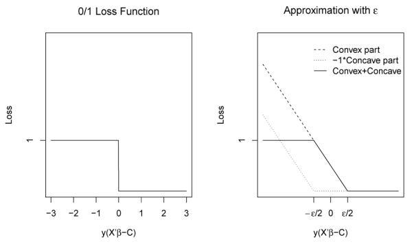
An illustration of using the difference between two hinge loss functions to approximate a 0/1 loss. A smaller ϵ provides a closer approximation.

The optimization is then performed by the concave-convex procedure proposed by Yuille and Rangarajan (2003). The concave-convex procedure relies on decomposing an objective function, f(x), into a convex part, f_∪(x), and a concave part, f_∩(x) such that

$$f\left(x\right)=f_{\cup }\left(x\right)+f_{\cap }\left(x\right).$$

Optimization is carried out with an iterative procedure in which f_∩(x) is linearized at the current solution x^(t),

$$x^{\left(t+1\right)}=\underset{x}{\arg \min }\left[f_{\cup }\left(x\right)+(x-x^{\left(t\right)})f_{\cap }^{\prime }\left(x^{\left(t\right)}\right)\right],$$

making each iteration a convex optimization problem. The first value x⁽⁰⁾ can be initialized with any reasonable guess.

To apply the concave-convex procedure to our optimization problem, we define the first term in Equation (5) as f_∪(β) and the second term as f_∩(β). The gradient of the concave part, f_∩(β), is

$$\frac{\partial f_{\cap }\left(\beta \right)}{\partial \beta }=\{\begin{array}{cc}\sum _{i=1}^n{w}_i\left(\frac{1}{ϵ}{y}_i{X}_i^{\prime }\right)\hfill & \text{if}\frac{1}{2}+\frac{1}{ϵ}{y}_i\left(X_i^{\prime }\beta -C_i\right)<0\hfill \\ 0\hfill & \text{if}\frac{1}{2}+\frac{1}{ϵ}{y}_i\left(X_i^{\prime }\beta -C_i\right)>0\hfill \end{array}\phantom{\}}$$

Applying the concave-convex procedure to the above decomposition, we obtain

$$\begin{array}{cc}\hfill {\beta }^{\left(r+1\right)}& =\underset{\beta }{\arg \min }\{\sum _{i=1}^n{w}_i{\left[\frac{1}{2}-\frac{1}{ϵ}{y}_i\left(X_i^{\prime }\beta -C_i\right)\right]}_{+}\phantom{\}}\hfill \\ \hfill & \phantom{\{}+\sum _{i=1}^n{w}_i\frac{1}{ϵ}{y}_i{X}_i^{\prime }\left(\beta -{\beta }^{\left(r\right)}\right)\cdot I\left[\frac{1}{2}+\frac{1}{ϵ}{y}_i(X_i^{\prime }{\beta }^{\left(r\right)}-C_i)<0\right]\},\hfill \end{array}$$ (6)

where β^(r) denotes the estimated β at the rth iteration. The final form can be solved with a standard convex optimization algorithm with a decreasing sequence of ϵ = {2⁰, 2⁻¹, ⋯}. Specifically, the initial values for both the simulation studies and the real data example were generated using a coarse grid search. Given the initial value, we solve Equation (6) with ϵ = 2⁰. The solution with ϵ = 2⁰ is then used as the initial value to solve Equation (6) with ϵ = 2⁻¹. This is repeated until the maximum relative change over all covariates is less than one percent. In this study, the fminsearch function from the optimization toolbox in MATLAB was used to solve for β. The fminsearch function performs unconstrained nonlinear optimization to find the minimum of a scalar function of several variables.

2.3. Inference

The confidence intervals for parameter estimates are obtained using a subsampling method since the bootstrap does not consistently estimate the asymptotic distribution for estimators with cube-root convergence (Abrevaya and Huang 2005). The subsampling method described below is from Politis et al. (1999). Subsampling can produce consistent estimated sampling distributions under extremely weak assumptions even when the bootstrap fails and it can be used to obtain confidence intervals for parameter estimates. It should not be used to obtain standard errors; however, since our estimators are not normally distributed, even asymptotically (Section 3.3); therefore, there is no simple relation between the distribution of the estimators and standard errors (Horowitz 2010, page 108). The justification for using the subsampling method in our study is discussed further in Section 3.3.

To obtain confidence intervals for the minimizer of Equation (5), ${\widehat{\beta }}_{n,ϵ}$, we produce subsamples K₁, K₂, ⋯ ,K_Nn where K_j’s are the $N_n\equiv \left(\begin{array}{c}\hfill n\hfill \\ \hfill b\hfill \end{array}\right)$ distinct subsets of {(C_i, X_i, δ_i)_{i=1,⋯ ,n}} of size b. Let β_τ denote the true parameter values and ${\widehat{\beta }}_{n,ϵ,b,j}$ denote the estimated value produced by solving Equation (6) using the K_jth dataset.

Define

$$L_{n,b}\left(x\right)=N_n^{-1}\sum _{j=1}^{N_n}I[b^{1∕3}\left({\widehat{\beta }}_{n,ϵ,b,j}-{\widehat{\beta }}_{n,ϵ}\right)\le x]\text{and}{c}_{n,b}\left(\gamma \right)=\inf \{x:L_{n,b}\left(x\right)\ge \gamma \}.$$

From Theorem 2.2.1 of Politis et al. (1999), for any 0 < γ < 1,

$$P\left[n^{1∕3}\left({\widehat{\beta }}_{n,ϵ}-{\beta }_{\tau }\right)\le c_{n,b}\left(\gamma \right)\right]\to \gamma ,$$

under the condition that b → ∞ as n → ∞ and b/n → 0. It follows that for any 0 < α < 1 ,

$$P\left[c_{n,b}\left(\frac{\alpha }{2}\right)<n^{1∕3}\left({\widehat{\beta }}_{n,ϵ}-{\beta }_{\tau }\right)\le c_{n,b}\left(1-\frac{\alpha }{2}\right)\right]\to 1-\alpha$$

thus an asymptotic 1 − α level confidence interval for β_τ can be constructed with

$$\left[{\widehat{\beta }}_{n,ϵ}-n^{-1∕3}{c}_{n,b}\left(1-\frac{\alpha }{2}\right),{\widehat{\beta }}_{n,ϵ}-n^{-1∕3}{c}_{n,b}\left(\frac{\alpha }{2}\right)\right].$$

Symmetric confidence intervals can be obtained by modifying the above approach slightly. Define

$${\tilde{L}}_{n,b}\left(x\right)=N_n^{-1}\sum _{j=1}^{N_n}I[b^{1∕3}\mid {\widehat{\beta }}_{n,ϵ,b,j}-{\widehat{\beta }}_{n,ϵ}\mid \le x]\text{and}{\tilde{c}}_{n,b}\left(\gamma \right)=\inf \{x:{\tilde{L}}_{n,b}\left(x\right)\ge \gamma \}.$$

Again, if b → ∞ as n → ∞ and at the same time b/n → 0, a symmetric confidence interval for β_τ can be constructed as

$$\left[{\widehat{\beta }}_{n,ϵ}-n^{-1∕3}{\tilde{c}}_{n,b}\left(1-\alpha \right),{\widehat{\beta }}_{n,ϵ}+n^{-1∕3}{\tilde{c}}_{n,b}\left(1-\alpha \right)\right].$$ (7)

Symmetric confidence intervals are desirable because they often have nicer properties than the nonsymmetric version in finite samples (Banerjee and Wellner 2005). This fact was also observed in our simulation studies; hence, symmetric confidence intervals are recommended and used in this paper.

To avoid large scale computation issues, a stochastic approximation from Politis et al. (1999) is employed where B randomly chosen datasets from {1, 2, ⋯ ,N_n} are used in the above calculation. Furthermore, the block size is chosen using the method implemented in Delgado et al. (2001) and Banerjee and Wellner (2005). Briefly, the algorithm for choosing block size is described below.

Step 1

Fix a selection of reasonable block sizes b between limits b_low and b_up.

Step 2

Draw M bootstrap samples from the actual dataset.

Step 3

For each bootstrap sample, construct a subsampling symmetric confidence interval with asymptotic coverage 1 − α for each block size b. Let R_m,b be one if ${\widehat{\beta }}_{n,ϵ}$ was within the mth interval based on block size b and zero otherwise.

Step 4

Compute $\widehat{h}\left(b\right)=M^{-1}{\sum }_{m=1}^M{R}_{m,b}$.

Step 5

Find the value $\tilde{b}$ that minimizes $\mid \widehat{h}\left(b\right)-\alpha \mid$ and use $\tilde{b}$ as the block size when constructing confidence interval for the original data.

3. ASYMPTOTIC PROPERTIES

3.1. Identifiability

Prior to deriving the asymptotic properties of the proposed estimator, we will discuss a set of sufficient conditions for identifiability. For a fixed quantile τ, let

$$Z_n\left(\beta \right)=\frac{1}{n}\sum _{i=1}^n\left[\tau I\left({\delta }_i=0\right)I\right(X_i^{\prime }\beta -C_i\le 0)+\left(1-\tau \right)I\left({\delta }_i=1\right)I(X_i^{\prime }\beta -C_i>0\left)\right],$$

and

$$Z\left(\beta \right)=E[\tau I\left(\delta =0\right)I\left(X^{\prime }\beta -C\le 0\right)+\left(1-\tau \right)I\left(\delta =1\right)I\left(X^{\prime }\beta -C>0\right)].$$

Let β_τ denote a minimizer of Z(·). The following conditions will be used in subsequent theorems.

Condition 1

The support of f_X is not contained in any proper linear subspace of ${\Re }^k$.

Condition 2

f_T∣X(t) and f_C∣X(t) are continuous and positive in a neighborhood of X′β_τ with probability 1, where f_T∣X and f_C∣X are the conditional densities of T and C given X.

Condition 1 is the typical full-rank condition. Conditions 1 and 2 are sufficient for β_τ to be identifiable, as shown in the following lemma. Intuitively, the positivity of f_T∣X and f_C∣X in a neighborhood of t = X′β_τ ensures that the conditional probability of P(T ≤ t∣X) is estimable for t around its τ-quantile using current status data. In other words, the conditions make it possible to differentiate between Q_T(τ∣X) and Q_T(τ ± ϵ∣X) for a sufficiently small ϵ over a full ranked set of X.

Lemma 1

Under Conditions 1 and 2, β_τ is identifiable, i.e. β_τ is the unique minimizer of Z(·).

We prove Lemma 1 by showing Z(β)−Z(β_τ) > 0, ∀β ≠ β_τ. A detailed proof is provided in the Appendix.

3.2. Consistency

For a fixed quantile τ, let

$$\begin{array}{cc}\hfill Z_{n,ϵ}\left(\beta \right)=& \sum _{i=1}^n(\tau I\left({\delta }_i=0\right)\left\{I(X_i^{\prime }\beta -C_i\le -\frac{ϵ}{2})+I(\mid X_i^{\prime }\beta -C_i\mid <\frac{ϵ}{2})\left[-\frac{1}{ϵ}(X_i^{\prime }\beta -C_i-\frac{ϵ}{2})\right]\right\}\phantom{)}\hfill \\ \hfill & +\phantom{(}\left(1-\tau \right)I\left({\delta }_i=1\right)\left\{I(X^{\prime }\beta -C_i>\frac{ϵ}{2})+I(\mid X_i^{\prime }\beta -C_i\mid \le \frac{ϵ}{2})\left[\frac{1}{ϵ}(X_i^{\prime }\beta -C_i+\frac{ϵ}{2})\right]\right\})\hfill \end{array}$$

We assume the following conditions for the consistency theorem.

Condition 3

Let β_τ ∊ $\mathcal{B}$ where $\mathcal{B}$ is a compact subset of ${\Re }^k$ which contains β_τ as an interior point.

Condition 4

M_T ≡ sup_T,X f_T∣X(T ∣ X) < ∞ and M_C ≡ sup_C,X f_C∣X(C ∣ X) < ∞.

Let ${\widehat{\beta }}_{n,ϵ}$ be the minimizer of Z_n,ϵ(·) in $\mathcal{B}$.

Theorem 1

Under Conditions 1−4, ${\widehat{\beta }}_{n,ϵ}$ converges to β_τ in probability as n → ∞ and ϵ → 0.

The proof follows by first showing that the collection of functions in Z_n(β) is a VC-subgraph class and hence Z_n(β) converge almost surely uniformly to Z(β). In addition, Z_n,ϵ(β) converges almost surely uniformly to Z_n(β) as n → ∞ and ϵ → 0; thus we can conclude that Z_n,ϵ(β) converges almost surely uniformly to Z(β). Next, we prove that Z(·) is continuous. Conditions 1 and 2 provide sufficient conditions for identifiability and hence, β_τ is the unique minimizer of Z(·). Since we assumed $\mathcal{B}$ is compact, we can then conclude that ${\widehat{\beta }}_{n,ϵ}$ converges to β_τ in probability by a standard argument for M-estimators (Theorem 2.1 of Newey and McFadden (1994)). A detailed proof is provided in the Appendix.

3.3. Asymptotic Distribution

This section shows that $n^{1∕3}\left({\widehat{\beta }}_{n,ϵ}-{\beta }_{\tau }\right)$ converges to a nondegenerate distribution. The convergence rate is atypical because our objective function (4) is non-smooth and not everywhere differentiable; this is sometimes called the “sharp-edge effect” (Kim and Pollard 1990). We will need the following conditions in Theorem 2 to guarantee that the asymptotic distribution will be nondegenerate, namely

Condition 5

The ϵ of Equation (5) is o(n^−2/3).

Condition 6

The distribution C, T and X is absolutely continuous with respect to Lebesgue measure.

Condition 7

X is bounded.

Condition 8

Let V (β_τ)_i,j = P_x [X_iX_jf_C∣X(X′β_τ ∣ X)f_T∣X(X′β_τ ∣ X)] and V(β_τ) is positive definite where X_i and X_j are elements of X.

Theorem 2

Under Conditions 1−8, the process $\left\{n^{2∕3}[Z_n\left({\beta }_{\tau }+{\mathit{sn}}^{-1∕3}\right)-Z_n\left({\beta }_{\tau }\right)]:s\in {\Re }^k\right\}$ converges in distribution to a Gaussian process $\left\{\Gamma \left(s\right):s\in {\Re }^k\right\}$ with continuous sample paths, mean s′V (β_τ)s/2, and covariance H, where V is the second order expansion of Z(β) at β_τ, and

$$\begin{array}{cc}\hfill H\left(s,r\right)=& \underset{\alpha \to \infty }{\lim }\alpha P_{C,X}\{{[\tau -F_{T\mid X}\left(C\mid X\right)]}^2\phantom{\}}\hfill \\ \hfill & \phantom{\{}\left[I\left(\frac{X^{\prime }r\vee X^{\prime }s}{\alpha }<C-X^{\prime }{\beta }_{\tau }\le 0\right)+I\left(0<C-X^{\prime }{\beta }_{\tau }<\frac{X^{\prime }r\wedge X^{\prime }s}{\alpha }\right)\right]\}\hfill \end{array}$$

when it exists. Furthermore, $n^{1∕3}({\widehat{\beta }}_{n,ϵ}-{\beta }_{\tau }){\to }_d\arg \inf \Gamma \left(s\right)$.

Theorem 2 follows by verifying the conditions of the main theorem from Kim and Pollard (1990). Provided that V is positive definite, we can conclude that $n^{1∕3}({\widehat{\beta }}_{n,ϵ}-{\beta }_{\tau })$ converges to a nondegenerate distribution. A detailed proof is provided in Appendix.

Subsampling can produce consistent estimated sampling distributions for our estimator and it is an immediate consequence of Theorem 2.2.1 from Politis et al. (1999). In our study, we choose block size b = N^γ where γ = {1/3, 1/2, 2/3, 3/4, 0.8, 5/6, 6/7, 0.9, 12/13, 0.95} thus b → ∞ and b/N → 0 as N → ∞. $n^{1∕3}({\widehat{\beta }}_{n,ϵ}-{\beta }_{\tau })$ converges to a nondegenerate continuous distribution. All conditions in Theorem 2.2.1 from Politis et al. (1999) are met thus we can construct confidence intervals as stated in Section 2.3.

4. NUMERICAL STUDIES

4.1. Simulation

Two simulation studies were carried out to test the finite sample performance of our estimator. We used conditional quantile functions which were linear in the covariate for each study. In the first scenario, Simulation 1, the conditional quantile functions had identical linear coefficients and differed only in intercept. In the second scenario, Simulation 2, both the intercepts and covariate effects varied over the quantiles. Simulation 1 represents a situation where the errors are independent and identically distributed and Simulation 2 represents a situation where the errors are heteroscedastic.

In Simulation 1, the covariate is X ≡ (1, X₁, X₂)′ where X₁ ~ Uniform [0, 2] and X₂ ~ Bernoulli(0.5). The unobserved failure times, T, were generated from the linear model, T = 2 + 3X₁ + X₂ + 0.3 U. The observation times, C, were generated from the linear model, C = 1.9 + 3.2X₁ + 0.8 V when X₂ = 0 and C = 3.1 + 2.8X₁ + 0.8 V when X₂ = 1. Both U and V were generated from N(0, 1). The proportion of events occurring prior to the observation time (δ = 1) was about 50%. The underlying 0.25 quantile is Q_T (0.25∣X) = 1.798 + 3X₁ + X₂, the underlying 0.50 quantile is Q_T (0.50∣X) = 2 + 3X₁ + X₂, and the underlying 0.75 quantile is Q_T(0.75∣X) = 2.202 + 3X₁ + X₂. Since it is possible that T and/or C are negative, in a survival analysis context, we can treat T and C as the logarithm of survival time and logarithm of observation time, respectively.

In Simulation 2, the covariate setup is the same as in Simulation 1. Unobserved failure times were generated from the linear model, T = 2+3X₁ + X₂ +(0.2+0.5X₁) U and the observation times, C, were generated from the linear model C = 1.8 + 3.2X₁ + 0.8X₂ + 0.8 V . Both U and V were generated from exponential distribution with rate equal to one. The proportion of events occurring prior to the observation time (δ = 1) was about 50%. The underlying 0.25 quantile is Q_T(0.25∣X) = 2.058 + 3.144X₁ + X₂, the underlying 0.50 quantile is Q_T(0.50∣X) = 2.139 + 3.347X₁ + X₂, and the underlying 0.75 quantile is Q_T(0.75∣X) = 2.277 + 3.693X₁ + X₂.

We are interested in estimation of the 0.25 quantile, median, and 0.75 quantile. For each scenario, we reported the mean bias, mean squared error, and median absolute deviation based on 1000 simulations. Sample sizes were chosen to be n = 200, 400, and 800 for each simulation setup. Since the unobserved event time, T, and the observation time, C, were generated as a function of covariates and the error terms were generated from distributions which had positive density in the neighborhood of quantiles of interests, our simulation setup satisfy the identifiability conditions in Lemma 1.

For each simulated dataset, the procedure described at the end of Section 2.2 was used to estimate β. Symmetric confidence intervals as in Equation (7) were calculated based on a stochastic approximation with 500 subsamples. To decrease computational burdens, the block size was determined via a pilot simulation in the same fashion as described in Banerjee and McKeague (2007). In a small scale simulation study, we examined the block size chosen by the algorithm described in Section 2.3 and by the pilot simulation method described in Banerjee and McKeague (2007). The block sizes chosen by either method produced similar average coverage which indicated the coverage presented in this section is a good representation of the coverage when confidence intervals are constructed using the algorithm described in Section 2.3. The optimal subsampling block size was determined from the following selected block sizes: {n^1/3, n^1/2, n^2/3, n^3/4, n^0.8, n^5/6, n^6/7, n^0.9, n^12/13, n^0.95}.

Table 1 and Table 2 summarize the results for Simulation 1 and Simulation 2 with sample size equal to 200, 400, and 800 at the 0.25, median, and 0.75 quantiles. In the tables, “Truth” is the true parameter value; “Bias” is the mean bias of the estimates from all replicates; “MSE” is the mean squared error; “MAD” is the median absolute deviation of the estimates; “CP” is the average coverage from subsampling symmetric confidence intervals; and “Length” is the average confidence interval length. The tables show that the regression coefficient estimators have negligible bias.

Table 1.

Simulation results for Simulation 1, based on 1000 simulation replicates.

N	τ	Parameter	Truth	Bias	MSE	MAD	CP	Length
200	0.25	β 0	1.798	0.026	0.036	0.117	0.921	0.679
		β 1	3.000	−0.010	0.022	0.097	0.941	0.542
		β 2	1.000	0.020	0.028	0.110	0.923	0.604
	0.50	β 0	2.000	0.002	0.032	0.120	0.931	0.633
		β 1	3.000	−0.006	0.018	0.088	0.946	0.500
		β 2	1.000	0.012	0.025	0.106	0.935	0.547
	0.75	β 0	2.202	−0.011	0.039	0.138	0.925	0.695
		β 1	3.000	−0.010	0.023	0.100	0.931	0.544
		β 2	1.000	0.010	0.029	0.109	0.927	0.602
400	0.25	β 0	1.798	0.007	0.020	0.097	0.942	0.530
		β 1	3.000	−0.002	0.012	0.074	0.958	0.415
		β 2	1.000	0.009	0.018	0.094	0.943	0.476
	0.50	β 0	2.000	−0.004	0.017	0.083	0.940	0.472
		β 1	3.000	0.002	0.010	0.066	0.944	0.372
		β 2	1.000	0.006	0.014	0.074	0.938	0.423
	0.75	β 0	2.202	−0.005	0.020	0.098	0.945	0.527
		β 1	3.000	−0.001	0.012	0.074	0.950	0.411
		β 2	1.000	−0.002	0.016	0.087	0.939	0.473
800	0.25	β 0	1.798	0.006	0.012	0.074	0.942	0.403
		β 1	3.000	−0.001	0.007	0.057	0.946	0.315
		β 2	1.000	0.002	0.010	0.068	0.941	0.365
	0.50	β 0	2.000	−0.003	0.010	0.065	0.939	0.367
		β 1	3.000	0.001	0.006	0.049	0.958	0.288
		β 2	1.000	0.004	0.009	0.062	0.944	0.338
	0.75	β 0	2.202	−0.005	0.012	0.073	0.937	0.406
		β 1	3.000	0.003	0.007	0.054	0.950	0.319
		β 2	1.000	−0.001	0.010	0.065	0.950	0.365

Truth is the true parameter value; Bias is mean of bias from 1000 replicates; MSE is mean squared error; MAD is median absolute deviation of the estimates; CP is the empirical coverage probabilities with a nominal level of 0.95 from subsampling symmetric confidence intervals with 500 subsamples; and Length is mean confidence interval length.

Table 2.

Simulation results for Simulation 2, based on 1000 simulation replicates.

N	τ	Parameter	Truth	Bias	MSE	MAD	CP	Length
200	0.25	β 0	2.058	0.003	0.039	0.073	0.934	0.759
		β 1	3.144	0.010	0.020	0.087	0.956	0.563
		β 2	1.000	0.042	0.038	0.090	0.942	0.749
	0.50	β 0	2.139	0.027	0.030	0.109	0.938	0.662
		β 1	3.347	0.014	0.035	0.123	0.930	0.657
		β 2	1.000	0.021	0.040	0.126	0.937	0.745
	0.75	β 0	2.277	0.059	0.082	0.166	0.931	0.973
		β 1	3.693	−0.031	0.099	0.203	0.908	1.037
		β 2	1.000	0.006	0.110	0.209	0.939	1.284
400	0.25	β 0	2.058	0.020	0.012	0.053	0.953	0.439
		β 1	3.144	0.001	0.008	0.059	0.955	0.358
		β 2	1.000	0.003	0.013	0.063	0.957	0.457
	0.50	β 0	2.139	0.025	0.016	0.079	0.949	0.480
		β 1	3.347	0.011	0.019	0.096	0.935	0.495
		β 2	1.000	0.006	0.022	0.094	0.940	0.550
	0.75	β 0	2.277	0.039	0.045	0.128	0.952	0.768
		β 1	3.693	−0.016	0.059	0.158	0.934	0.843
		β 2	1.000	0.012	0.062	0.160	0.950	0.924
800	0.25	β 0	2.058	0.014	0.004	0.040	0.957	0.272
		β 1	3.144	0.001	0.004	0.041	0.954	0.253
		β 2	1.000	0.001	0.006	0.050	0.955	0.299
	0.50	β 0	2.139	0.017	0.009	0.059	0.954	0.350
		β 1	3.347	0.000	0.010	0.068	0.940	0.373
		β 2	1.000	0.003	0.012	0.070	0.950	0.414
	0.75	β 0	2.277	0.026	0.024	0.103	0.968	0.595
		β 1	3.693	−0.002	0.036	0.126	0.942	0.676
		β 2	1.000	0.009	0.037	0.124	0.948	0.707

Truth is the true parameter value; Bias is mean of bias from 1000 replicates; MSE is mean squared error; MAD is median absolute deviation of the estimates; CP is the empirical coverage probabilities with a nominal level of 0.95 from subsampling symmetric confidence intervals with 500 subsamples; and Length is mean confidence interval length.

In Simulation 1, the bias has a decreasing trend as the sample size increases for all quantiles and parameters. The mean squared errors and median absolute deviations decrease as the sample size increases for all quantiles and parameters. The subsampling confidence interval coverage is slightly lower than the nominal 95% level in smallest sample size (N=200) but the empirical coverage probability is close to 95% as the sample size increases. In Simulation 2, the bias for all quantiles is small for all sample sizes. There is a general decreasing trend for bias when the sample size increases. The mean squared errors and median absolute deviations decrease as the sample size increases for all quantiles and parameters. The average 95% confidence interval coverage rate is a bit low for the smallest sample size (N=200) but gets closer to the nominal 0.95 level as the sample size increases. In both scenarios, the median absolute deviations for sample size 800 is roughly 63% of the median absolute deviation for sample size 200 which is consistent with the cube-root rate.

The algorithm seems to converge in all of our simulation studies. Nonconvergence of the algorithm would be an indication that the data might not have sufficient information to support the estimation at the specified quantile. The computation time to estimate one quantile for each of the 100 simulated dataset ranged from 30 to 42 seconds for sample sizes 200 to 800 using a computer equipped with an Intel(R) Core(TM) i5-2500 CPU @3.30GHz 3.60 GHz CPU and 4.00 GB RAM. The computation times are similar for the second simulation scenario.

To illustrate the strengths and limitations of the proposed method, an accelerated failure time (AFT) model with normally distributed errors was fit to the simulated datasets. Table 3 shows the results from the AFT models. In Table 3, the ‘truth’ column is the true parameter values for Simulation 1, and the mean from the accelerated failure time model with exponentially distributed errors for Simulation 2. When the error distribution in the AFT model is correctly specified, as in Simulation 1, the estimates have negligible bias. The true parameter values of the AFT model is the same as the true parameter value at the median because the Normal distribution is symmetric; therefore, the conditional mean is the same as the conditional median. Since the error terms are correctly specified, the parametric method has higher efficiency than the proposed method which can be seen from the much smaller confidence interval length. When the error distribution is incorrectly specified, as in Simulation 2, the estimates are alarmingly biased. The coverage percentage is low for β₂ and is extremely low for both β₀ and β₁ even though the confidence intervals are narrow. Our method has a lower efficiency than the parametric method when the error distribution can be correctly specified in the parametric method. On the other hand, when the error distribution is incorrectly specified in the parametric method, our proposed method clearly outperforms the parametric method in terms of unbiased estimation and retaining proper coverage levels. The strength of our proposed method lies in the fact that it is a semiparametric method thus we do not need to know the true underlying distribution of the error terms in the AFT model.

Table 3.

Results from accelerated failure time models with normal error, based on 1000 simulation replicates.

Simulation	N	Parameter	Truth	Bias	MSE	MAD	CP	Length
1	200	β 0	2.000	0.009	0.010	0.069	0.935	0.371
		β 1	3.000	−0.007	0.006	0.052	0.945	0.290
		β 2	1.000	0.001	0.008	0.057	0.933	0.332
	400	β 0	2.000	0.002	0.005	0.046	0.951	0.263
		β 1	3.000	−0.001	0.003	0.035	0.955	0.205
		β 2	1.000	−0.001	0.004	0.040	0.948	0.236
	800	β 0	2.000	−0.0004	0.002	0.033	0.954	0.187
		β 1	3.000	0.0001	0.001	0.024	0.948	0.146
		β 2	1.000	0.001	0.002	0.020	0.946	0.167
2	200	β 0	2.200	0.269	0.090	0.268	0.497	0.550
		β 1	3.500	0.326	0.119	0.323	0.149	0.426
		β 2	1.000	0.061	0.021	0.095	0.928	0.496
	400	β 0	2.200	0.281	0.088	0.283	0.185	0.389
		β 1	3.500	0.317	0.107	0.315	0.016	0.301
		β 2	1.000	0.056	0.011	0.071	0.913	0.351
	800	β 0	2.200	0.275	0.080	0.276	0.027	0.274
		β 1	3.500	0.318	0.105	0.318	0	0.212
		β 2	1.000	0.061	0.008	0.065	0.833	0.247

Truth is the true parameter value, in Simulation 1. Truth is the mean of an accelerated failure time with exponential distributed error, in Simulation 2 ; Bias is mean of bias from 1000 replicates; MSE is mean squared error; MAD is median absolute deviation of the estimates; CP is the empirical coverage probabilities with a nominal level of 0.95; and Length is mean confidence interval length.

4.2. Application

We applied the proposed method to analysis of the “Mayo Clinic Study of Aging” (MCSA) data. The detailed study design is described in Roberts et al. (2008). The results from a cross-sectional analysis (Jack et al. 2014) and a longitudinal analysis (Jack et al. 2016) have been published elsewhere. The MCSA is a longitudinal population-based study of cognitive aging in residents of Olmsted County, Minnesota, USA (Roberts et al. 2008). Four thousands and forty nine participants were enrolled and the follow-up visits occurred approximately every 15 months.

To understand the time to incidence of cognitive impairment, participants with clinically normal cognitive function and who had at least one follow-up visit (N=3388) were included in our analysis. The study was originally designed to understand the change of biomarkers for amyloidosis and neurodegeneration over time; thus, the follow-up visits occur regularly. To change the data structure into current status data, and to allow sufficient time for participants to develop cognitive impairment, we used the first available follow-up which was more than 2 years from the original observation to assess a patient’s current cognitive impairment status. In doing so, 759 participants who did not have a follow-up more than 2 years from their baseline observation were excluded. Additionally, 154 participants who had missing glucose levels at their baseline were also excluded since we are using it as one of the covariates in the model. The final analysis included 2,475 participants from the MCSA dataset aged 51-91 (median=74) of which 50.8% (N=1,258) were male.

Since we would like to understand the age of incidence for cognitive impairment, a participants’ age at the first follow-up more than 2 years from baseline was used as the response variable. Participants were between 53.4 and 94.2 years old (median=76.9 years old) at the first follow-up more than 2 years from baseline. Histograms for the age at the first follow-up more than 2 years from baseline for males and females are shown in Figure 2. There does not appear to be a difference in age between males and females at the first follow-up more than 2 years from baseline. In our analysis, the outcome “cognitive impairment” is defined as clinical diagnosis of either mild cognitive impairment or dementia at the follow-up visit. Among 2,475 participants, 240 (9.7%) were diagnosed with cognitive impairment by the first follow-up visit at least 2 years from baseline (136 males and 104 females). The (unobserved) failure time of interest was the age of incident cognitive impairment. The analysis examined the effect of gender and glucose level at baseline on the quantiles of age to cognitive impairment.

Figure 2.

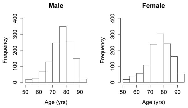
Age at first follow-up more than 2 years from baseline for 2,475 participants in MCSA.

Before applying our proposed method on the data, we need to determine for which quantiles the regression coefficients are estimable. Following the remark in Section 3.1, it was sufficient to examine which quantiles of T can be estimated well using current status data over all covariate values. Thus, a nonparametric maximum likelihood estimator (NPMLE) of the (unobserved) failure time distribution function was fit to the data stratified by the covariates (Wellner and Zhan 1997; Gentleman and Vandal 2011). The NPMLE can tell us whether data provides enough information for estimation of a certain quantile. Moreover, Turnbull (1976) noted that the NPMLE was not unique within certain intervals. The shady areas in the NPMLE figure represent the non-unique areas. A large shaded area is an indication that the data might not contain enough information for estimation; thus, we should avoid estimating quantiles within a large non-unique area. Specifically, the distribution estimator in Figure 3 suggests that the data may provide enough information for estimation for quantiles less than 0.3 for males since the cumulative probability for incidence of cognitive impairment does not rise above 0.3. Therefore, we focused only on 0.10 to 0.25 quantiles with increments of 0.05 when performing data analysis. We centered the glucose level at 96 mg/dL (median) then divided it by 10. Our proposed model was fitted for the lower quantiles and symmetric confidence intervals were constructed by subsampling where the block size was chosen based on the algorithm presented in Section 2.3. The results are summarized in Table 4 and Figure 4.

Figure 3.

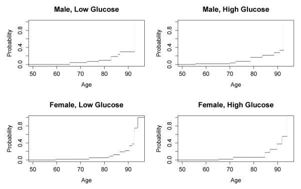
Nonparametric maximum likelihood estimator (NPMLE) of the (unobserved) failure time distribution function stratified by gender and glucose level (below or above median).

Table 4.

Results of analyzing “Mayo Clinic Study of Aging” data, effect on age of incident cognitive impairment.

Quantile	Parameter	Estimate	Lower C.I.	Upper C.I.
0.10	Intercept	83.350	81.083	85.617
	Male vs. Female	−4.045	−6.938	−1.151
	(Glucose – 96)/10	−0.926	−2.245	0.392
0.15	Intercept	87.331	84.474	90.188
	Male vs. Female	−3.123	−6.162	−0.084
	(Glucose – 96)/10	−1.599	−3.195	−0.003
0.20	Intercept	88.244	85.856	90.632
	Male vs. Female	−2.673	−5.680	0.334
	(Glucose – 96)/10	−0.532	−1.872	0.808
0.25	Intercept	90.148	87.097	93.198
	Male vs. Female	−2.494	−6.376	1.388
	(Glucose – 96)/10	−0.210	−2.021	1.601

Figure 4.

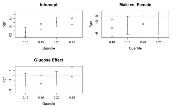
MCSA data: effect on age of incident cognitive impairment. The vertical bars are symmetric confidence interval constructed using a subsampling method.

The results indicate that the 0.10, 0.15, 0.20, and 0.25 quantiles for the incidence of cognitive impairment for a female with a glucose level of 96 mg/dL would be 83.4, 87.3, 88.2, and 90.1 years old, respectively. Compared to females, the onset of cognitive impairment for male participants is 4 years earlier at the 0.10 quantile and the effect diminishes in magnitude at higher quantiles. The negative effect of male is statistically significant at 0.10 and 0.15 quantiles but became insignificant at the higher quantiles. Elevated glucose levels also had a negative effect on age of incidence for cognitive impairment. The magnitude of glucose effects are similar at all quantiles examined. Each 10 mg/dL increase in glucose level is associated with around 1 ~ 2 years earlier onset of cognitive impairment for the 0.1 and 0.15 quantiles and around 0.5 year earlier onset for 0.20 and 0.25 quantiles. The effect of glucose level is statistically significant only at the 0.15 quantile.

Quantile regression models provided additional insights toward risk factors associated with incidence cognitive impairment. The gender differences in mild cognitive impairment and dementia have been documented in the literatures (Roberts et al. 2012; Ruitenberg et al. 2001). Using quantile regression, we can describe the differential gender effect over different quantiles in a quantitative manner. Male participants have earlier onset at lower quantiles (i.e. younger age) but the effect dissipates at higher quantiles (i.e. older age). The association between glucose level and dementia is also recognized (Crane et al. 2013). The similar point estimates for glucose levels across quantiles suggest that the glucose effect may be a simple shift in the distribution for the age of incidence for cognitive impairment.

5. DISCUSSION

To solve the non-convex objective function in Equation (4), we used the difference between two convex hinge functions Equation (5) to approximate the objective function. One practical issue is how to choose a good initial value, since a good initial value is critical to prevent the algorithm from stalling at an unsuitable local minimum. Currently, we used a coarse grid search to generate the initial value. A grid search can be done in low dimensional data but it is not practical when the data is high dimensional. Further work is needed to investigate a practical method to produce reasonable initial values for high dimensional data.

In real data analysis, it may be the case that not all quantiles are estimable. It is not due to the estimation procedure but the sparse data structure. Consider a situation where a disease requires a long incubation period, if the observation times are all concentrated in a short period, most subjects would not have developed any symptoms yet. We will have most people with δ = 0 at the end of the observation period. In this case, the higher tail quantiles will not be estimable because we simply do not have enough information. We recommend to obtain a NPMLE of the cumulative density function stratified by covariates as we did for the MCSA data. The NPMLE results can provide useful information about which quantiles can be reasonably estimated.

The method proposed in this paper can be easily extended to Case 2 interval-censored data. For example, suppose the event occurred in interval (L,R], we can simply treat this as 2 records in the current status data format. The first record would have C = L, and δ = 0 and the second record would have C = R, and δ = 1 then the same optimization routine can be carried out for estimation. In the interval (L,R], either L may be 0 or R may be ∞ (having both L = 0 and R = ∞ would mean that no information was supplied by the observation). Extension to right censored data may be possible. Intuitively, the non-censored observations can be treated as the event occurred within a very small interval and right-censored observation can be treated as current status with C equal to the censoring time and δ = 0. This extension will not require the “global linearity assumption” which is commonly assumed in existing quantile regression models for rightcensoring data (Portnoy 2003; Peng and Huang 2008). The validity of this extension will need careful examination and analytic appraisal before trusting. Furthermore, models with varying coefficients or nonparametric quantile regression models may be useful for practical purposes which warrant future investigation.

Appendix A. Appendix

Proof of lemma and theorems

Proof of Lemma 1.

$$\begin{array}{cc}\hfill Z\left(\beta \right)& -Z\left({\beta }_{\tau }\right)=P_{C,X}[\left\{\tau I\left(\delta =0\right)I\left(X^{\prime }\beta \le C\right)+\left(1-\tau \right)I\left(\delta =1\right)I\left(X^{\prime }\beta >C\right)\right\}\phantom{]}\hfill \\ \hfill & -\phantom{[}\left\{\tau I\left(\delta =0\right)I\left(X^{\prime }{\beta }_{\tau }\le C\right)+\left(1-\tau \right)I\left(\delta =1\right)I\left(X^{\prime }{\beta }_{\tau }>C\right)\right\}]\hfill \\ \hfill & =P_{C,X}\left[\{\tau I\left(\delta =0\right)-\left(1-\tau \right)I\left(\delta =1\right)\}\left\{I\left(X^{\prime }\beta \le C<X^{\prime }{\beta }_{\tau }\right)-I\left(X^{\prime }{\beta }_{\tau }\le C<X^{\prime }\beta \right)\right\}\right]\hfill \\ \hfill & =P_{C,X}\left[\{\tau -I\left(\delta =1\right)\}\left\{I\left(X^{\prime }\beta \le C<X^{\prime }{\beta }_{\tau }\right)-\left(X^{\prime }{\beta }_{\tau }\le C<X^{\prime }\beta \right)\right\}\right]\hfill \\ \hfill & =P_{C,X}\left[\{\tau -F_{T\mid X}\left(C\mid X\right)\}\left\{I\left(X^{\prime }\beta \le C<X^{\prime }{\beta }_{\tau }\right)-I\left(X^{\prime }{\beta }_{\tau }\le C<X^{\prime }\beta \right)\right\}\right]\hfill \\ \hfill & ={\int }_X{\int }_{C\mid X}\{\tau -F_{T\mid X}\left(C\mid X\right)\}\left\{I\left(X^{\prime }\beta \le C<X^{\prime }{\beta }_{\tau }\right)-I\left(X^{\prime }{\beta }_{\tau }\le C<X^{\prime }\beta \right)\right\}{\mathit{dP}}_{C\mid X}{\mathit{dP}}_X\hfill \\ \hfill & ={\int }_X{\int }_{\left(X^{\prime }\beta \le c<X^{\prime }{\beta }_{\tau }\right)\bigcup \left(X^{\prime }{\beta }_{\tau }\le c<X^{\prime }\beta \right)}\mid {\int }_{X^{\prime }{\beta }_{\tau }}^c{f}_{T\mid X}\left(t\right)f_{C\mid X}\left(c\right)\mathit{dt}\mid \mathit{dc}{\mathit{dP}}_X\hfill \end{array}$$

When β ≠ β_τ, there is a positive probability that the set {(X′β ≤ c < X′β_τ)⋃(X′β_τ ≤ c < X′β) is not empty. Furthermore, Condition 2 ensures that f_T∣X and f_C∣X are positive for c near X′β_τ. Thus, there is a positive probability that the inner most integral is positive. We then conclude that, Z(β) − Z(β_τ) > 0 for all β ≠ β_τ and hence, β_τ is identifiable.

Remark

It is true that the derivative of Z(β) with respect to β is zero at the true β. Z(β) is defined as

$$\begin{array}{cc}\hfill Z\left(\beta \right)& =E\left\{\tau I\left(\delta =0\right)I\left(X^{\prime }\beta -C\le 0\right)+\left(1-\tau \right)I\left(\delta =1\right)I\left(X^{\prime }\beta -C>0\right)\right\}\hfill \\ \hfill & ={\int }_X\left({\int }_{X^{\prime }\beta }^{\infty }\tau {\mathit{dF}}_{C\mid X}+{\int }_0^{X^{\prime }\beta }{F}_{T\mid X}\left(c\right){\mathit{dF}}_{C\mid X}-\tau {\int }_0^{\infty }{F}_{T\mid X}\left(c\right){\mathit{dF}}_{C\mid X}\right){\mathit{dF}}_X.\hfill \end{array}$$

We can take the derivative of Z(β) with respect to β as,

$$\frac{\partial }{\partial \beta }Z\left(\beta \right)={\int }_X\{-\tau f_{C\mid X}\left(X^{\prime }\beta \right)X+F_{T\mid X}\left(X^{\prime }\beta \right)f_{C\mid X}\left(X^{\prime }\beta \right)X\}{\mathit{dF}}_X.$$

By definition, F_T∣X(X′β_τ) = τ , so it is immediate that $\frac{\partial }{\partial \beta }Z\left(\beta \right){\mid }_{\beta ={\beta }_{\tau }}=0$.

Proof of Theorem 1

We shall prove this theorem by showing

$$\underset{\beta \in \mathcal{B}}{\sup }\mid Z_{n,ϵ}\left(\beta \right)-Z\left(\beta \right)\mid \to 0\text{almost surely}$$ (A.1)

and then showing Z(β) is continuous. By Lemma 1, β_τ is the unique minimizer of Z(·) and since $\mathcal{B}$ is assumed, we can use Theorem 2.1 of Newey and McFadden (1994) to conclude that ${\widehat{\beta }}_{n,ϵ}\to {\beta }_{\tau }$ in probability.

We can show Equation (A.1) is true by proving

$$\underset{\beta \in \mathcal{B}}{\sup }\mid Z_n\left(\beta \right)-Z\left(\beta \right)\mid \to 0\text{almost surely},\underset{\beta \in \mathcal{B}}{\sup }\mid Z_{n,ϵ}\left(\beta \right)-Z_n\left(\beta \right)\mid \to 0\text{almost surely}$$

since

$$\underset{\beta \in \mathcal{B}}{\sup }\mid Z_{n,ϵ}\left(\beta \right)-Z\left(\beta \right)\mid \le \underset{\beta \in \mathcal{B}}{\sup }\mid Z_{n,ϵ}\left(\beta \right)-Z_n\left(\beta \right)\mid +\underset{\beta \in \mathcal{B}}{\sup }\mid Z_n\left(\beta \right)-Z\left(\beta \right)\mid$$ (A.2)

The class of indicator functions I(δ = 0), I(δ = 1), ${\mathcal{I}}_1\equiv \{I\left(X^{\prime }\beta -C\le 0\right):\beta \in \mathcal{B}\}$, and ${\mathcal{I}}_2\equiv \{I\left(X^{\prime }\beta -C>0\right):\beta \in \mathcal{B}\}$ are examples of Vapnik-C̆ervonenkis (VC)-subgraph classes. τ and 1−τ are fixed functions and thus by Lemma 2.6.18 (i) and (vi) of van der Vaart and Wellner (1996), the classes $\tau I\left(\delta =0\right){\mathcal{I}}_1$ and $\left(1-\tau \right)I\left(\delta =1\right){\mathcal{I}}_2$ are also VC-subgraph classes. Finally, (v) of the same lemma gives that $\mathcal{Z}\equiv \{Z_n\left(\beta \right):\beta \in \mathcal{B}\}$ is a VC-subgraph class. Since $\mathcal{Z}$ is a VC-subgraph class, it is also a Glivenko-Cantelli class; hence, ${\sup }_{\beta \in \mathcal{B}}\mid Z_n\left(\beta \right)-Z\left(\beta \right)\mid \to 0$ almost surely.

Since $I(\mid X_i^{\prime }\beta -C_i\mid \le ϵ∕2)$ is a VC class of functions, ${\mathbf{P}}_n\left\{I\right(\mid X_i^{\prime }\beta -C_i\mid \le ϵ∕2\left)\right\}$ converges to $P\left\{I\right(\mid X_i^{\prime }\beta -C_i\mid \le ϵ∕2\left)\right\}$ uniformly over $\mathcal{B}$ where P_n is the empirical measure and P is the true underlying measure. Thus, we have

$$\begin{array}{cc}\hfill \underset{\beta \in \mathcal{B}}{\sup }\mid Z_{n,ϵ}\left(\beta \right)-Z_n\left(\beta \right)\mid & \le \underset{\beta \in \mathcal{B}}{\sup }{\mathbf{P}}_n\left\{I\right(\mid X_i^{\prime }\beta -C_i\mid \le ϵ∕2\left)\right\}\hfill \\ \hfill & \underset{n\uparrow \infty }{\to }\underset{\beta \in \mathcal{B}}{\sup }P\left\{I\left(\mid X^{\prime }\beta -C\mid \le ϵ∕2\right)\right\}\hfill \\ \hfill & =\underset{\beta \in \mathcal{B}}{\sup }{P}_X{P}_{C\mid X}\left(\mid X^{\prime }\beta -C\mid \le ϵ∕2\mid X\right)\hfill \\ \hfill & \le P_X\left(ϵM_C\mid X\right)=ϵM_C\hfill \end{array}$$ (A.3)

By Condition 4, Equation (A.3) is bounded and converges to 0 as ϵ → 0, thus we can conclude that ${\sup }_{\beta \in \mathcal{B}}\mid Z_{n,ϵ}\left(\beta \right)-Z_n\left(\beta \right)\mid \to 0$ almost surely as n → ∞ and ϵ → 0.

Since each term on the right hand side of Equation (A.2) converges to 0 almost surely, we can conclude that ${\sup }_{\beta \in \mathcal{B}}\mid Z_{n,ϵ}\left(\beta \right)-Z\left(\beta \right)\mid \to 0$ almost surely as n → ∞ and ϵ → 0.

To show that Z(·) is continuous, we re-express Z(·) as

$$\begin{array}{cc}\hfill Z\left(\beta \right)& =E\left\{\tau I\left(\delta =0\right)I\left(X^{\prime }\beta -C\le 0\right)+\left(1-\tau \right)I\left(\delta =1\right)I\left(X^{\prime }\beta -C>0\right)\right\}\hfill \\ \hfill & ={\int }_X\left[\tau {\int }_{X^{\prime }\beta }^{\infty }\{1-F_{T\mid X}\left(c\right)\}{\mathit{dF}}_{C\mid X}+\left(1-\tau \right){\int }_0^{X^{\prime }\beta }{F}_{T\mid X}\left(c\right){\mathit{dF}}_{C\mid X}\right]{\mathit{dF}}_X\hfill \\ \hfill & ={\int }_X\left({\int }_{X^{\prime }\beta }^{\infty }\tau {\mathit{dF}}_{C\mid X}+{\int }_0^{X^{\prime }\beta }{F}_{T\mid X}\left(c\right){\mathit{dF}}_{C\mid X}-\tau {\int }_0^{\infty }{F}_{T\mid X}\left(c\right){\mathit{dF}}_{C\mid X}\right){\mathit{dF}}_X.\hfill \end{array}$$ (A.4)

Only the first two inner integrals are functions of β. Under Condition 4, both of these inner integrals are bounded and continuous with respect to β; therefore, Z(·) is continuous.

Proof of Theorem 2

Before proceeding with the proof, we will state the main theorem from Kim and Pollard (1990). The theorem concerns estimators defined by minimization of process ${\mathbf{P}}_{n}g\left(\cdot ,\theta \right)=\frac{1}{n}{\sum }_{i\le n}g\left({\xi }_i,\theta \right)$, where {ξ_i} is a sequence of independent observations taken from a distribution P and {g(·, θ) : θ ∊ Θ} is a class of functions indexed by a subset Θ of ${\Re }^d$. P_n denotes the expectation with respect to the empirical process. The envelope G_R(·) is defined as the supremum of ∣g(·, θ)∣ over the class g_R = {g(·, θ) : ∣θ − θ_o∣ ≤ R} .

Kim and Pollard (1990)

Let {θ_n} be a sequence of estimators for which (i) P_ng(· , θ_n) ≤ inf_θ∊Θ P_ng(·, θ) + o_p(n^−2/3).

Suppose

(ii) θ_n converges in probability to the unique θ₀ that minimizes Pg(·, θ);

(iii) θ₀ is an interior point of Θ.

Let the functions be standardized so that g(·, θ₀) ≡ 0. If the classes g_R, for R near 0, are uniformly manageable for the envelopes G_R and satisfy

(iv) Pg(·, θ) is twice differentiable with second derivative matrix V at θ₀;

(v) H(s, t) = lim_α→∞ αPg(·, θ₀ + s/α)g(·, θ₀ + t/α) exists for each s, t in ${\Re }^d$ and

$$\underset{\alpha \to \infty }{\lim }\alpha \mathit{Pg}{(\cdot ,{\theta }_0+t∕\alpha )}^{2}I\{\mid g\left(\cdot ,{\theta }_0+t∕\alpha \right)\mid >ϵ\alpha \}=0$$

for each ϵ > 0 and t in ${\Re }^d$;

(vi) ${\mathit{PG}}_R^2=O\left(R\right)$ as R → 0 and for each ϵ > 0 there is a constant K such that ${\mathit{PG}}_R^{2}I\{G_R>K\}<ϵR$ for R near 0;

(vii) P∣g(·, θ₁) − g(·, θ₂)∣ = O(∣θ₁ − θ₂∣) near θ₀; then the process n^2/3P_ng(·, θ₀ + tn^−1/3) converges in distribution to a Gaussian process Z(t) with continuous sample paths, expected value t′V t/2 and covariance kernel H.

If V is positive definite and if Z has nondegenerate increments, then n^1/3(θ_n − θ₀) converges in distribution to the (almost surely unique) random vector that minimizes Z(t).

Now we proceed with our proof of theorem 2. It will be convenient to define a version of the original objective function centered at the true value β_τ ,

$$\begin{array}{cc}\hfill g\left(\beta \right)& =\left\{\tau I\left(\delta =0\right)I\left(X^{\prime }\beta \le C\right)+\left(1-\tau \right)I\left(\delta =1\right)I\left(X^{\prime }\beta >C\right)\right\}\hfill \\ \hfill & -\left\{\tau I\left(\delta =0\right)I\left(X^{\prime }{\beta }_{\tau }\le C\right)+\left(1-\tau \right)I\left(\delta =1\right)I\left(X^{\prime }{\beta }_{\tau }>C\right)\right\}\hfill \\ \hfill & =\{\tau I\left(\delta =0\right)-\left(1-\tau \right)I\left(\delta =1\right)\}\left\{I\left(X^{\prime }\beta \le C<X^{\prime }{\beta }_{\tau }\right)-I\left(X^{\prime }{\beta }_{\tau }\le C<X^{\prime }\beta \right)\right\}\hfill \\ \hfill & =\{\tau -I\left(\delta =1\right)\}\left\{I\left(X^{\prime }\beta \le C<X^{\prime }{\beta }_{\tau }\right)-I\left(X^{\prime }{\beta }_{\tau }\le C<X^{\prime }\beta \right)\right\}.\hfill \end{array}$$

Under the true distribution P, we haveP(g(β)) = Z(β) − Z(β_τ). The minimum value of P(g(·)) is then obtained at the arg min of Z(·) and P(g(β_τ)) = 0. The estimator we use here is ${\widehat{\beta }}_{n,ϵ}$ which is the minimizer of Z_n,ϵ(·) defined as in (5).

The first condition of the main theorem from Kim and Pollard (1990) is satisfied under Condition 5. By the definition of ${\widehat{\beta }}_{n,ϵ}$, we have $Z_{n,ϵ}\left({\widehat{\beta }}_{n,ϵ}\right)\le \underset{\beta }{\inf }{Z}_{n,ϵ}\left(\beta \right)+o_p\left(n^{-2∕3}\right)$. We also have $Z_n\left({\widehat{\beta }}_{n,ϵ}\right)-{\inf }_{\beta }{Z}_n\left(\beta \right)\ge 0$ by definition.

$$\begin{array}{cc}\hfill Z_n\left({\widehat{\beta }}_{n,ϵ}\right)-\underset{\beta }{\inf }{Z}_n\left(\beta \right)& \le Z_{n,ϵ}\left({\widehat{\beta }}_{n,ϵ}\right)+{\mathbf{P}}_n\left\{I\left(\mid C-X^{\prime }{\beta }_{n,ϵ}\mid <ϵ∕2\right)\right\}\hfill \\ \hfill & -\underset{\beta \in \beta }{\inf }\left[Z_{n,ϵ}\left(\beta \right)-{\mathbf{P}}_n\left\{I\left(\mid C-X^{\prime }\beta \mid <ϵ∕2\right)\right\}\right]\hfill \\ \hfill & \le Z_{n,ϵ}\left({\widehat{\beta }}_{n,ϵ}\right)-\underset{\beta }{\inf }{Z}_{n,ϵ}\left(\beta \right)+2\underset{\beta }{\sup }{\mathbf{P}}_n\left\{I\left(\mid C-X^{\prime }\beta \mid <ϵ∕2\right)\right\}\hfill \\ \hfill & \le Z_{n,ϵ}\left({\widehat{\beta }}_{n,ϵ}\right)-\underset{\beta }{\inf }{Z}_{n,ϵ}\left(\beta \right)+2\underset{\beta }{\sup }P\left(\mid C-X^{\prime }\beta \mid <ϵ∕2\right)+o_p\left(ϵn^{-1∕2}\right)\hfill \\ \hfill & \le Z_{n,ϵ}\left({\widehat{\beta }}_{n,ϵ}\right)-\underset{\beta }{\inf }{Z}_{n,ϵ}\left(\beta \right)+2ϵM_C+o_p\left(n^{-7∕6}\right)=o_p\left(n^{-2∕3}\right)\hfill \end{array}$$

Therefore, $Z_n\left({\widehat{\beta }}_{n,ϵ}\right)\le {\inf }_{\beta }{Z}_n\left(\beta \right)+o_p\left(n^{-2∕3}\right)$ which satisfied the first condition. The second condition, ${\widehat{\beta }}_{n,ϵ}\to {\beta }_{\tau }$ in probability, has been verified in Theorem 1. The third condition is satisfied by assuming Condition 2.

The remaining four conditions of the theorem deal with the nature of expectation of g under the measure P. P(g) may be expressed as

$$\begin{array}{cc}\hfill P\left(g\left(\beta \right)\right)& =P\left[\{\tau -I\left(\delta =1\right)\}\left\{I\left(X^{\prime }\beta \le C<X^{\prime }{\beta }_{\tau }\right)-I\left(X^{\prime }{\beta }_{\tau }\le C<X^{\prime }\beta \right)\right\}\right]\hfill \\ \hfill & =P_{C,X}\left\{P\left[\right\{\tau -I\left(\delta =1\right)\}\mid C,X]\left\{I\left(X^{\prime }\beta \le C<X^{\prime }{\beta }_{\tau }\right)-I\left(X^{\prime }{\beta }_{\tau }\le C<X^{\prime }\beta \right)\right\}\right\}\hfill \\ \hfill & =P_{C,X}\left[\{\tau -F_{T\mid X}\left(C\mid X\right)\}\left\{I\left(X^{\prime }\beta \le C<X^{\prime }{\beta }_{\tau }\right)-I\left(X^{\prime }{\beta }_{\tau }\le C<X^{\prime }\beta \right)\right\}\right]\hfill \end{array}$$

where F_T∣X(· ∣ ·) is the conditional distribution of T given X. This expectation is dominated by:

$$\begin{array}{cc}\hfill P\mid g\left(\beta \right)\mid & =P\mid \{\tau -F_{T\mid X}\left(C\mid X\right)\}\left\{I\left(X^{\prime }\beta \le C<X^{\prime }{\beta }_{\tau }\right)-I\left(X^{\prime }{\beta }_{\tau }\le C<X^{\prime }\beta \right)\right\}\mid \hfill \\ \hfill & \le P\left\{I\left(X^{\prime }\beta \le C<X^{\prime }{\beta }_{\tau }\right)+I\left(X^{\prime }{\beta }_{\tau }\le C<X^{\prime }\beta \right)\right\}\le 1.\hfill \end{array}$$

Since P is absolutely continuous with respect to Lebesgue measure, for any sequence d_n → 0, the dominated convergence theorem tells us P(g(β+d_n)) → P(g(β)). In other words, P(g(β)) is continuous with respect to β.

We may expand P(g(β)) with a Taylor expansion. The first derivative is found by interchanging integration (expectation) and differentiation to find

$$\begin{gathered} \frac{\partial }{\partial {\beta }_i}P\left(g\left(\beta \right)\right) \\ ={\int }_X\left\{\tau -F_{T\mid X}\left(X^{\prime }\beta \mid X\right)\right\}{X}_i{f}_{C\mid X}\left(X^{\prime }\beta \mid X\right)\{-I\left(X^{\prime }\beta <X^{\prime }{\beta }_{\tau }\right)-I\left(X^{\prime }{\beta }_{\tau }<X^{\prime }\beta \right)\}\mathit{dP} \\ ={\int }_X\left\{F_{T\mid X}\left(X^{\prime }\beta \mid X\right)-\tau \right\}{X}_i{f}_{C\mid X}\left(X^{\prime }\beta \mid X\right){\mathit{dP}}_X, \end{gathered}$$

where f_C∣X is the density of the observation time C conditioned on X and X_i is an element of X_i. Evaluated at β_τ, the term F_T∣X(β_τX ∣ X) − τ equal to zero by definition of the τth quantile, making the derivative equal zero as would be expected for an extrema. Taking one step further, the second derivative would be

$$\begin{gathered} V{(\beta )}_{i,j}=\frac{{\partial }^2}{\partial {\beta }_i\partial {\beta }_j}P\left(g(\beta )\right) \\ ={\int }_X\left(F_{T\mid X}\left(X^{\prime }\beta \mid X\right)-\tau \right)X_i{X}_j\frac{\partial }{\partial C}{f}_{C\mid X}\left(X^{\prime }\beta \mid X\right){\mathit{dP}}_X \\ +{\int }_X{X}_i{X}_j{f}_{C\mid X}\left(X^{\prime }\beta \mid X\right)f_{T\mid X}\left(X^{\prime }\beta \mid X\right){\mathit{dP}}_X. \end{gathered}$$

At β_τ , the first integral vanishes and only the second remains taking the form

$$V{\left({\beta }_{\tau }\right)}_{i,j}={\int }_X\left\{X_i{X}_j{f}_{C\mid X}\left(X^{\prime }{\beta }_{\tau }\mid X\right)f_{T\mid X}\left(X^{\prime }{\beta }_{\tau }\mid X\right)\right\}{\mathit{dP}}_X$$

As the entries are dominated by

$$\mid V{\left({\beta }_{\tau }\right)}_{i,j}\mid \le M_C{M}_T{M}_{\mid X\mid }^2,$$

where M_∣X∣ is the bound over all ∣X_i∣ and M_C and M_T are defined in Condition 4. V (β_τ)_i,j will be well defined verifying the fourth condition of the theorem. Writing

$$V\left({\beta }_{\tau }\right)=P_X\left({\mathit{XX}}^{\prime }h\left(X\right)\right),\text{with}h\left(X\right)=f_{C\mid X}\left(X^{\prime }\beta \mid X\right)f_{T\mid X}\left(X^{\prime }\beta \mid X\right)\ge 0,$$

show that V (β_τ) would be a symmetric positive semi-definite matrix since it is a positive mixture of the positive semi-definite terms XX′. A sufficient condition for V (β_τ) to be positive definite is that the Lebesgue measure of the set {X : f_C∣X(X′β_τ ∣ X)f_T∣X(X′β_τ ∣ X)f_X(X) > 0} is greater than zero.

To able control asymptotic covariance of Z(s), let

$$\begin{gathered} H\left(s,r\right)=\underset{\alpha \to \infty }{\lim }\alpha P\left\{g\left({\beta }_{\tau }+r∕\alpha \right)g\left({\beta }_{\tau }+s∕\alpha \right)\right\} \\ =\underset{\alpha \to \infty }{\lim }\alpha P_{C,X}\{{\{\tau -F_{T\mid X}\left(C\mid X\right)\}}^2\phantom{\}} \\ \left[I\{X^{\prime }\left({\beta }_{\tau }+r∕\alpha \right)\le C<X^{\prime }{\beta }_{\tau }\}-I\{X^{\prime }{\beta }_{\tau }\le C<X^{\prime }\left({\beta }_{\tau }+r∕\alpha \right)\}\right] \\ \left[I\{X^{\prime }\left({\beta }_{\tau }+s∕\alpha \right)\le C<X^{\prime }{\beta }_{\tau }\}-I\{X^{\prime }{\beta }_{\tau }\le C<X^{\prime }\left({\beta }_{\tau }+s∕\alpha \right)\}\right] \\ =\underset{\alpha \to \infty }{\lim }\alpha P_{C,X}[{\{\tau -F_{T\mid X}\left(C\mid X\right)\}}^2\phantom{]} \\ \phantom{[}\left\{I\left(\frac{X^{\prime }r\vee X^{\prime }s}{\alpha }\le C-X^{\prime }{\beta }_{\tau }<0\right)+I\left(0\le C-X^{\prime }{\beta }_{\tau }<\frac{X^{\prime }r\wedge X^{\prime }s}{\alpha }\right)\right\}], \end{gathered}$$

where ⋁ and ⋀ denote maximum and minimum, respectively. Using Condition 4 and 7, we have

$$\begin{gathered} P_{C,X} \\ [{\{\tau -F_{T\mid X}\left(C\mid X\right)\}}^2\left\{I\left(\frac{X^{\prime }r\vee X^{\prime }s}{\alpha }\le C-X^{\prime }{\beta }_{\tau }<0\right)+I\left(0\le C-X^{\prime }{\beta }_{\tau }<\frac{X^{\prime }r\wedge X^{\prime }s}{\alpha }\right)\right\}\phantom{]} \\ \le {\int }_X{M}_C\frac{\mid X^{\prime }r\mid \wedge \mid X^{\prime }s\mid }{\alpha }{\mathit{dP}}_X\le M_C\frac{\left({\Vert s\Vert }_1+{\Vert r\Vert }_1\right)M_{\mid X\mid }}{\alpha }=O\left({\alpha }^{-1}\right), \end{gathered}$$

hence, along with Condition 6, H(s, r) is well defined by the dominated convergence theorem satisfying the fifth condition.

Let G_R be the envelope of ${\mathbf{g}}_R\equiv \{g\left(\beta \right):{\Vert \beta -{\beta }_{\tau }\Vert }_{\infty }<R\le \widetilde{ϵ}\}$, i.e.,

$$G_R=\mid \tau -I\left(\delta =1\right)\mid I\left(\mid C-X^{\prime }{\beta }_{\tau }\mid <R\max \mid X_j\mid \right)\le I\left(\mid C-X^{\prime }{\beta }_{\tau }\mid <R\max \mid X_j\mid \right)$$

A sufficient condition for the class g_R to be uniformly manageable is that its envelope function G_R is uniformly square integrable given that {g(β)} is VC-subgraph (Mohammadi and Van De Geer 2005). Since G_R is bounded by one, it is uniformly square integrable for R close to zero. Together with the fact that {g(β)} is VC-subgraph, we conclude that g_R is uniformly manageable.

Then

$$\begin{gathered} P\left(G_R^2\right)\le {\int }_X{\int }_{\Re }I\left(\mid C-X^{\prime }{\beta }_{\tau }\mid <R\max \mid X_j\mid \right){\mathit{dP}}_{C\mid X}{\mathit{dP}}_X \\ \le {\int }_{X}2M_{C}R\max \left(\mid X_j\mid \right){\mathit{dP}}_X\le R\left(2M_C{M}_{\mid X\mid }\right)=O\left(R\right). \end{gathered}$$

For any ϵ > 0, we can use K = 2, then $E\left\{G_R^{2}I\left(G_R>K\right)\right\}=0<ϵR$ since G_R is less than K everywhere. Combining these two traits satisfying the sixth condition of the theorem.

The final condition is verified by letting G_R,β be the envelope of $\{g\left(\tilde{\beta }\right)-g\left(\beta \right):{\Vert \tilde{\beta }-\beta \Vert }_{\infty }<R\}$, i.e.,

$$G_{R,\beta }=\mid \tau -I\left(\delta =1\right)\mid I\left(\mid C-X^{\prime }\beta \mid <R\max \mid X_j\mid \right)\le I\left(\mid C-X^{\prime }\beta \mid <R\max \mid X_j\mid \right).$$

Using the same integration inequalities as used in the preceding for G_R we find that $P\mid g\left(\tilde{\beta }\right)-g\left(\beta \right)\mid =O\left({\Vert \tilde{\beta }-\beta \Vert }_{\infty }\right)=O\left({\Vert \tilde{\beta }-\beta \Vert }_1\right)$ over all β, $\tilde{\beta }$ in an $\widetilde{ϵ}$ neighborhood of β_τ since ∥ · ∥_∞ and ∥ · ∥₁ are equivalent metrics.

As the seven conditions are satisfied, the conclusion of the main theorem in Kim and Pollard (1990) follows which in turn proved Theorem 2.

References

- Abrevaya J, Huang J. On the bootstrap of the maximum score estimator. Econometrica. 2005;73(4):1175–1204. [Google Scholar]
- Banerjee M, McKeague IW. Confidence sets for split points in decision trees. The Annals of Statistics. 2007;35(2):543–574. [Google Scholar]
- Banerjee M, Wellner JA. Confidence intervals for current status data. Scandinavian Journal of Statistics. 2005;32(3):405–424. [Google Scholar]
- Buchinsky M, Hahn J. An alternative estimator for the censored quantile regression model. Econometrica. 1998;66(3):653–671. [Google Scholar]
- Cade BS, Noon BR. A gentle introduction to quantile regression for ecologists. Frontiers in Ecology and the Environment. 2003;1(8):412–420. [Google Scholar]
- Chernozhukov V, Hong H. Three-step censored quantile regression and extramarital affairs. Journal of the American Statistical Association. 2002;97(459):872–882. [Google Scholar]
- Crane PK, Walker R, Hubbard RA, Li G, Nathan DM, Zheng H, Haneuse S, Craft S, Montine TJ, Kahn SE, et al. Glucose levels and risk of dementia. New England Journal of Medicine. 2013;369(6):540–548. doi: 10.1056/NEJMoa1215740. [DOI] [PMC free article] [PubMed] [Google Scholar]
- Delgado MA, Rodriguez-Poo JM, Wolf M. Subsampling inference in cube root asymptotics with an application to manskis maximum score estimator. Economics Letters. 2001;73(2):241–250. [Google Scholar]
- Gentleman R, Vandal A. Icens: NPMLE for Censored and Truncated Data. R package version 1.24.0 2011. [Google Scholar]
- Honore B, Khan S, Powell JL. Quantile regression under random censoring. Journal of Econometrics. 2002;109(1):67–105. [Google Scholar]
- Horowitz J. Springer Series in Statistics. Springer; New York: 2010. Semiparametric and Nonparametric Methods in Econometrics. [Google Scholar]
- Huang Y. Quantile calculus and censored regression. Annals of Statistics. 2010;38(3):1607–1637. doi: 10.1214/09-aos771. [DOI] [PMC free article] [PubMed] [Google Scholar]
- Jack CR, Therneau TM, Wiste HJ, Weigand SD, Knopman DS, Lowe VJ, Mielke MM, Vemuri P, Roberts RO, Machulda MM, et al. Transition rates between amyloid and neurodegeneration biomarker states and to dementia: a population-based, longitudinal cohort study. The Lancet Neurology. 2016;15(1):56–64. doi: 10.1016/S1474-4422(15)00323-3. [DOI] [PMC free article] [PubMed] [Google Scholar]
- Jack CR, Wiste HJ, Weigand SD, Rocca WA, Knopman DS, Mielke MM, Lowe VJ, Senjem ML, Gunter JL, Preboske GM, et al. Age-specific population frequencies of cerebral β-amyloidosis and neurodegeneration among people with normal cognitive function aged 50–89 years: a cross-sectional study. The Lancet Neurology. 2014;13(10):997–1005. doi: 10.1016/S1474-4422(14)70194-2. [DOI] [PMC free article] [PubMed] [Google Scholar]
- Kim J, Pollard D. Cube root asymptotics. The Annals of Statistics. 1990;18(1):191–219. [Google Scholar]
- Kim Y-J, Cho H, Kim J, Jhun M. Median regression model with interval censored data. Biometrical Journal. 2010;52(2):201–208. doi: 10.1002/bimj.200900111. [DOI] [PubMed] [Google Scholar]
- Koenker R. Econometric Society Monographs. Cambridge University Press; 2005. Quantile Regression. [Google Scholar]
- Koenker R, Bassett, Gilbert J. Regression quantiles. Econometrica. 1978;46(1):33–50. [Google Scholar]
- Koenker R, Hallock KF. Quantile regression. Journal of Economic Perspectives. 2001;15(4):143–156. [Google Scholar]
- McKeague IW, Subramanian S, Sun Y. Median regression and the missing information principle. Journal of nonparametric statistics. 2001;13(5):709–727. [Google Scholar]
- Mohammadi L, Van De Geer S. Asymptotics in empirical risk minimization. The Journal of Machine Learning Research. 2005;6:2027–2047. [Google Scholar]
- Newey WK, McFadden D. Chapter 36 large sample estimation and hypothesis testing. In: Engle RF, McFadden DL, editors. Handbook of Econometrics. Vol. 4 of Handbook of Econometrics. Elsevier; 1994. pp. 2111–2245. [Google Scholar]
- Peng L. Self-consistent estimation of censored quantile regression. Journal of Multivariate Analysis. 2012;105(1):368–379. [Google Scholar]
- Peng L, Huang Y. Survival analysis with quantile regression models. Journal of the American Statistical Association. 2008;103(482):637–649. doi: 10.1198/016214508000000184. [DOI] [PMC free article] [PubMed] [Google Scholar]
- Politis D, Romano J, Wolf M. Springer series in statistics. Springer; 1999. Subsampling. [Google Scholar]
- Portnoy S. Censored regression quantiles. Journal of the American Statistical Association. 2003;98(464):1001–1012. doi: 10.1198/01622145030000001007. [DOI] [PMC free article] [PubMed] [Google Scholar]
- Powell JL. Least absolute deviations estimation for the censored regression model. Journal of Econometrics. 1984;25(3):303–325. [Google Scholar]
- Powell JL. Censored regression quantiles. Journal of Econometrics. 1986;32(1):143–155. [Google Scholar]
- Powell JL. Estimation of semiparametric models. Handbook of econometrics. 1994;4:2443–2521. [Google Scholar]
- Roberts R, Geda Y, Knopman D, Cha R, Pankratz V, Boeve B, Tangalos E, Ivnik R, Rocca W, Petersen R. The incidence of mci differs by subtype and is higher in men the mayo clinic study of aging. Neurology. 2012 doi: 10.1212/WNL.0b013e3182452862. WNL–0b013e3182452862. [DOI] [PMC free article] [PubMed] [Google Scholar]
- Roberts RO, Geda YE, Knopman DS, Cha RH, Pankratz VS, Boeve BF, Ivnik RJ, Tangalos EG, Petersen RC, Rocca WA. The mayo clinic study of aging: design and sampling, participation, baseline measures and sample characteristics. Neuroepidemiology. 2008;30(1):58–69. doi: 10.1159/000115751. [DOI] [PMC free article] [PubMed] [Google Scholar]
- Ruitenberg A, Ott A, van Swieten JC, Hofman A, Breteler MM. Incidence of dementia: does gender make a difference? Neurobiology of aging. 2001;22(4):575–580. doi: 10.1016/s0197-4580(01)00231-7. [DOI] [PubMed] [Google Scholar]
- Sun J. Statistics for Biology and Health. Springer; 2007. The Statistical Analysis of Interval-censored Failure Time Data. [Google Scholar]
- Turnbull BW. The empirical distribution function with arbitrarily grouped, censored and truncated data. Journal of the Royal Statistical Society. Series B (Methodological) 1976:290–295. [Google Scholar]
- van der Vaart A, Wellner J. Springer Series in Statistics. Springer; 1996. Weak Convergence and Empirical Processes: With Applications to Statistics. [Google Scholar]
- Wang HJ, Wang L. Locally weighted censored quantile regression. Journal of the American Statistical Association. 2009;104(487):1117–1128. [Google Scholar]
- Wellner JA, Zhan Y. A hybrid algorithm for computation of the nonparametric maximum likelihood estimator from censored data. Journal of the American Statistical Association. 1997;92(439):945–959. [Google Scholar]
- Yang S. Censored median regression using weighted empirical survival and hazard functions. Journal of the American Statistical Association. 1999;94(445):137–145. [Google Scholar]
- Ying Z, Jung SH, Wei LJ. Survival analysis with median regression models. Journal of the American Statistical Association. 1995;90(429):178–184. [Google Scholar]
- Yuille AL, Rangarajan A. The concave-convex procedure. Neural Comput. 2003 Apr.15(4):915–936. doi: 10.1162/08997660360581958. [DOI] [PubMed] [Google Scholar]