Semi-automated, single-band peak-fitting analysis of hydroxyl radical nucleic acid footprint autoradiograms for the quantitative analysis of transitions

Abstract

Hydroxyl radical footprinting can probe the solvent accessibility of the ribose moiety of the individual nucleotides of DNA and RNA. Semi-automated analytical tools are presented for the quantitative analyses of nucleic acid footprint transitions in which processes such as folding or ligand binding are followed as a function of time or ligand concentration. Efficient quantitation of the intensities of the electrophoretic bands comprising the footprinting reaction products is achieved by fitting a series of Lorentzian curves to line profiles obtained from gels utilizing sequentially relaxed constraints consistent with electrophoretic mobility. An automated process of data ‘standardization’ has been developed that corrects for differences in the loading amounts in the electrophoresis. This process enhances the accuracy of the derived transitions and makes generating them easier. Together with visualization of the processed footprinting in false-color two-dimensional maps, DNA and RNA footprinting data can be accurately, precisely and efficiently processed allowing transitions to be objectively and comprehensively analyzed. The utility of this new analysis approach is illustrated by its application to the ion-meditated folding of a large RNA molecule.

INTRODUCTION

‘Footprinting’ refers to assays in which either cleavage of the backbone or modification of the base or side-chain of a macromolecular polymer by a solution probe detects local differences in solvent accessibility (1). Many nucleic acid footprinting techniques utilize cleavage of the phosphodiester backbone with the reaction products detected by acrylamide gel electrophoretic separation and autoradiography. While visual inspection of resultant autoradiograms can yield much qualitative insight into the structure or ligand binding of a DNA or RNA molecule, accurate quantitation of ‘footprints’ can yield a wealth of information about equilibrium and kinetic transitions [reviewed in (2)].

Protocols were developed for the analysis of quantitative DNase I footprint titration autoradiograms that involved enveloping a band or series of bands on a gel within a contour (a ‘block’), integrating the optical density within the contour and correcting for the background of the autoradiogram. Transformations termed ‘standardization’ and ‘normalization’, respectively, are conducted for a series of lanes that comprise a titration experiment that correct for lane-to-lane density variation and convert density changes to apparent saturation (1,3,4).

Footprinting with hydroxyl radicals is a proven probe of the structure and function of DNA and RNA (5–8). Advantages of the hydroxyl radical as a nucleic acid footprinting probe include (i) sequence-independent intrinsic cleavage at each nucleotide, (ii) equivalent intrinsic reactivity towards single- and double-stranded structures and (iii) fine structural resolution due to the small size of the probe. The available evidence indicates that the hydroxyl radical cleaves the carbon backbone of the deoxyribose and ribose sugars, respectively, by hydrogen abstraction and subsequent ring opening as a function of the solvent accessibility of ring carbons (9,10). The autoradiograms of the hydroxyl radical reaction products are characterized by a ladder of bands corresponding to the products of n, n + 1, n + 2, n + 3, … nucleotides (Figures 1A and 9A) that place great demands on quantitative analysis protocols. While the ‘block’ approach to autoradiogram quantitation is effective for quantitating groups of bands or discontinuous cleavage patterns, it is both time-consuming to conduct and of limited precision for a band-by-band analysis.

Figure 1.

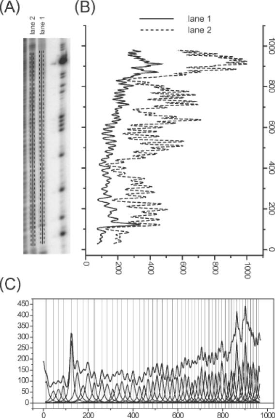
An overview of the peak-fitting procedure. (A) A portion of the phosphor storage image of a hydroxyl radical footprint of RNA. The ImageQuant software was used to draw the lines that define the line density profiles shown in (B). The dashed lines on either side of the solid one denote the horizontal boundaries of each line; the software averages the pixel density values of pixels between these boundaries for each vertical increment in the line profile. Lanes 1 and 2 differ by the presence of MgCl₂ in lane 2 to fold the RNA into a discrete tertiary structure. (B) The line profiles showing the average density for each row of pixels up the line from the bottom to the top of the gel. (C) The fit of the line profile for lane 1 to a family of Lorentzian curves as described in the text. Each Lorentzian peak corresponds to an individual band.

Figure 9.

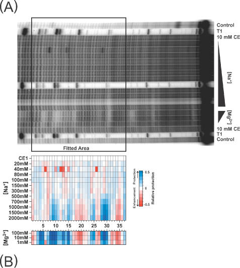
(A) An autoradiogram of part of a hydroxyl radical footprinting 8% gel of ³²P-labeled Tetrahymena group I ribozyme P4–P6 domain equilibrated under different NaCl concentrations and the native folded form equilibrated in Mg²⁺. The peak profiles were obtained and processed within the boxed area. (B) False-color representation of the resultant map generated using the protocols described in this paper.

A variety of ‘peak fitting’ protocols have been published that deconvolute a line scan of the banding pattern into a family of Gaussian or Lorentzian curves [e.g. (11–14)]. The combination of ‘peak fitting’ band density determinations with ‘standardization’ and ‘normalization’ data transformations in a semi-automated protocol is driven by the need to objectively extract high-resolution structural information at the single band level from transitions monitored by hydroxyl radical footprinting including new approaches that report time-dependent transitions on millisecond (15–18) or longer (19–21) timescales. An integrated peak-fitting approach is described in this paper that was developed for the analysis of the monovalent-ion-induced equilibrium folding of the ribozyme derived from the group 1 intron of Tetrahymena thermophila (22). The software that has been developed to implement this approach will be available for download on the corresponding author's webpage (http://www.aecom.yu.edu/mbrenowitz/).

MATERIALS AND METHODS

Biochemical protocols

Hydroxyl radical footprinting

The L-21 Sca1 ribozyme derived from the group 1 intron of T.thermophila was made by in vitro transcription, purified and then end labeled at either the 3′ or 5′ end with ³²P as described (15,23). RNA samples were annealed in the indicated buffer and exposed to hydroxyl radicals generated using either Fe-EDTA (7,8,24,25) or synchrotron radiation (16,26) as indicated in the text for a duration sufficient to achieve ‘single hit’ backbone cleavage kinetics. The samples were processed and separated by electrophoresis on 8% polyacrylamide, 5% bis-acrylamide gels using the TBE/Urea buffer system (6,27). The dried gels were imaged by exposure to a phosphor storage screen that was scanned with 16 bit image depth at 200 μm spatial resolutions with a Storm 820 imager (Molecular Dynamics™).

Computational protocols

Commercial software often contains useful graphical interfaces and powerful features that are difficult and expensive to duplicate. For this reason, our protocols use commercially available software when feasible and make use of scripting languages to implement special applications and tools. Processes that do not require a graphical interface can be implemented as command line C language programs to maximize the speed of their execution.

Acquisition of ‘lane profiles’

A profile of each lane of a gel (Figure 1A) is obtained from the digital autoradiogram using the ImageQuant software as has been described previously (14). Line profile generation is readily implemented in other software packages. Because of the high signal-to-noise of the phosphor storage plate image, the background density of the digital image is usually negligible (<0.5% of the peak band densities) and thus requires no processing. If the background is significant relative to the band densities, a baseline can be set at the averaged background level in the peak-fitting session.

In this procedure, a line (or ‘polyline’ if the lane is not straight) is drawn down the middle of a lane. The ‘width’ of the line is increased to ∼50% of the average width of the bands. This procedure averages the density across the relatively constant portion of the bands (Figure 1B). The data are exported to a spreadsheet as a two-dimensional array in the format of pixel intensity (arbitrary units) versus pixel number.

Peak fitting

The two-dimensional array of pixel intensity versus number is copied into the Origin v6.1 software equipped with the Peak Fitting Module v6.0 (OriginLab®). The peak-fitting operations are CPU intensive so that a fast processor and generous system and memory are desirable. A Windows 2000 workstation equipped with 1.5 GHz Pentium 4 processor and 384 MB RDRAM was used for the calculations presented in this article. In general, fitting 80–90 peaks requires 5–10 min on this system. The Lorentzian peak function is used since it adequately represents the shape of electrophoresis bands (12). The Lorentzian peak function is expressed as

where w_n is the peak width, A_n the peak area, xc_n the peak center position, n the peak number and (2A_n)/(πw_n) the peak height. Deconvolution of the lane profile is accomplished by nonlinear least-squares fitting to an array of Lorentzian peak functions (12,28) (Figure 1C). Portions of this procedure are automated as described in Results using the scripting language LabTalk™ within Origin. An outline of the procedure is as follows:

1. The initial guess for the peak center positions are manually assigned using the Peak Fitting Module Graphical Interface.

2. A LabTalk™ script performs several initialization operations. First, it selects a linear base line (consistent with uniform background of the phosphor storage screens). Second, the manually assigned peak center positions xc_n are improved by running a single iteration of the Peak Fitting Module's fitting routine. Third, the default values of w_n are discarded and new initial values that are proportional to the inter-peak distances are assigned (see Results, Equation 6).

3. The script then improves the quality of the initial guesses with the following iterative procedure. A single iteration of the nonlinear least-squares routine is performed with xc_n and w_n fixed (A_n only is floated) and the correlation coefficient recorded. Values of w_n are then increased by 1% (i.e. values of w_n are multiplied by 1.01) and the constrained fitting routine repeated. If the correlation coefficient improves, this operation is repeated until the correlation coefficient ceases to improve. If the correlation coefficient becomes worse, the values of w_n are decreased by 0.5% and the constrained fitting is repeated. This cycle of uniformly incrementing or decrementing the values of w_n is repeated ten times or until no improvement in the correlation coefficient is observed. This operation optimizes w_n within the model relating relative widths of the peaks encapsulated in Equation 6 (see Results). Its importance is that it minimizes excursions into local minima when the less constrained fitting in the next step is performed.

4. Following a review by the investigator of the fitting parameters assigned by the script in the preceding three steps, full fitting of the lane profile to a family of Lorentzian peaks is initiated. All of the peak parameters are floated (xc_n, A_n and w_n) with the constraints on w_n initially set to ±15% for first fitting session and then to ±5% for the subsequent fitting sessions (see next step). As discussed in the Results, the constraints on w_n required to achieve a physically meaningful fit of the model to the data depends upon the degree of peak separation.

5. The best-fit parameters of the first lane analyzed are saved as a template and imported as the initialization values for fitting the next lane. This procedure is effective since the peak parameters xc_n and w_n are well conserved across the lanes of a high-quality gel; only A_n will (incrementally) change during the course of a typical transition.

6. Steps (iii) and (iv) are repeated for the remainder of the lanes that constitute the transition curve being analyzed. The quantity sought in a line profile analysis, peak area, is expressed as

   

   where the parameters are as defined in Equation 1. The fitted peak areas (row i) determined for each lane of a gel (column j) are entered into the two-dimensional Peak Area Matrix A using a spreadsheet program (Figure 2A).

Figure 2.

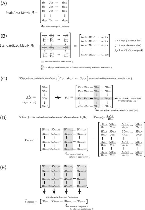
This figure outlines the matrices and transformations used to ‘standardize’ the data. (A) The ‘peak area matrix’ into which the results of the Lorentzian peak areas are transferred. (B) Within a peak area matrix, each row is divided by reference row a_k,j in order to convert to relative values independent of differences in the total intensity. This transformation, termed ‘standardization’, is repeated for each row resulting in a family of standardized matrices, A_k, for k = 1 → N where N is the total number of bands analyzed. (C) The standard deviation of each row for each matrix A_k and the values entered into the vector (k = 1 → N). The resultant vectors are assembled into the ‘standard deviation matrix’, V_i,k. Each row of this matrix presents the standard deviations of peak i standardized by each reference peak. (D) To compensate for the difference in standard deviations due to the original peak area, each column in matrix V_i,k is divided by the reference peak area that was used to calculate the standard deviations. The resultant is entered into the vectors that are assembled into the ‘normalized’ matrix V_norm,i,k. (E) The global standard deviation for each matrix A_k is calculated from the each column of V_norm,i,k and the resultant entered into the vector whose values are global measures of the quality of reference row k in A_k.

Automated data ‘standardization’

The first of two data transformations used to generate the equilibrium or time-dependent transitions monitored by footprinting (4) is ‘standardization’. The purpose of this transformation is to correct for variations in the amount of nucleic acid loaded onto each lane of a gel. Standardization ratios the fitted peak areas to a selected peak or peaks within the same lane. Ideally, a standard peak does not systematically vary with the transition being followed. In the context of RNA structure, optimum standard peaks are those whose solvent accessibility minimally changes throughout the transition being followed. The automated software iteratively tests each peak within a dataset as a candidate standard and presents the results in terms of the preferred rows in rank order for inspection by the investigator. The investigator then chooses the standard(s) to be used in the subsequent analysis of the data. The operations underlying this protocol will be considered in Results. The steps in this process are summarized below:

1. Peak Area Matrix A from step (v) above (Figure 2A) is the input into a program that calculates all of the possible Standardized Matrices A_k (k = 1 → N), where k is a candidate standard row and N is the total number of rows in the dataset, by dividing each element in Peak Area Matrix A by the corresponding element of row k (Figure 2B). This operation performs an unbiased testing of each row as a valid standard and avoids the assignment of standards based upon preconceptions about the structure of the nucleic acid or the behavior of a peak during the observed transition.

2. The standard deviation of each row of a Standardized Matrix A_k is calculated for the k = 1 → N family of matrices by

   

   where i and k are as defined above and r denotes the reference lane chosen for the transition. The results of this calculation are assembled into the Standard Deviation Matrix V_i,k (Figure 2C). This operation quantifies the variance of peaks in each row in Standardized Matrix A_k following its division by a candidate reference peak k.

3. Each column k in matrix V_i,k is divided by a designated element in reference lane r of the corresponding matrix A_k in order to normalize the values and the quotient entered into the Normalized standard deviation matrix V_norm,i,k where i and k are as defined above (Figure 2D). This operation corrects for differences in the relative peak areas among the columns in Standardized peak area matrix. For example, a row with large peaks might have a larger uncorrected standard deviation than a row with smaller ones despite having less variation (see Supplementary Material).

4. Each column in matrix V_norm,i,k is the standard deviation calculated for each row of Standardized Matrices A_k (Figure 2C). These data are collected into a Global standard deviation vector by calculation of the standard deviation of each of the columns in V_norm,i,k for k = 1 → N (Figure 2E). This operation provides a single measure of the overall variability of the rows of the Standardized Matrices A_k.

5. A score, Sc_k, is calculated for each candidate standard k that ranks the quality of each peak as a ‘standard’ by

   

   where 〈SD_norm,k〉 is the mean value of column k of the normalized standard deviation matrix V_norm,i,k. The rationale for this calculation and the use of this parameter is discussed in Results.

6. The investigator selects the standardized matrices A_k with the top five ‘scores’ for completion of the data reduction, visualization and analysis protocols describe below.

Calculation of relative protection

Visualization of the standardized data on a common scale is either the final step in their analysis or as a prelude to further quantitative analysis. ‘Normalization’ of the data to ‘apparent saturation’, , scales the relative peak areas to a reference condition that is defined as zero and represents one of the transition endpoints (3). The expression used is

where a_k,i,j is target element, a_k,i,n,r is the element of reference lane r in the row i. The reference lane is typically either the initial or final state of the transition being followed. This procedure converts units that are specific to a detection method (such as peak area) to a scale that is intuitive with respect to the biological system under investigation. Decreases in the reactivity of the footprinting probe relative to the reference (i.e. ‘protection’) yield values ranging from zero to one. Increases in the reactivity of the footprinting probe (i.e. ‘enhancement’) relative to the reference results in negative numbers. The normalization protocol is conducted on the Standardized Matrices A_k as follows:

1. All of the elements in the selected matrices are normalized to the elements in the reference lane using Equation 5 (Figure 3B).

2. The resultant normalized matrices A_k1 to A_k5 are then averaged to yield a single normalized averaged matrix A_norm (Figure 3C) that is output as a tab-delimited text file to ease importation into a spreadsheet application for subsequent visualization and analysis of the data. This matrix is the final result of the peak-fitting analysis and is the basis for data visualization or subsequent analysis of footprinting transitions.

Figure 3.

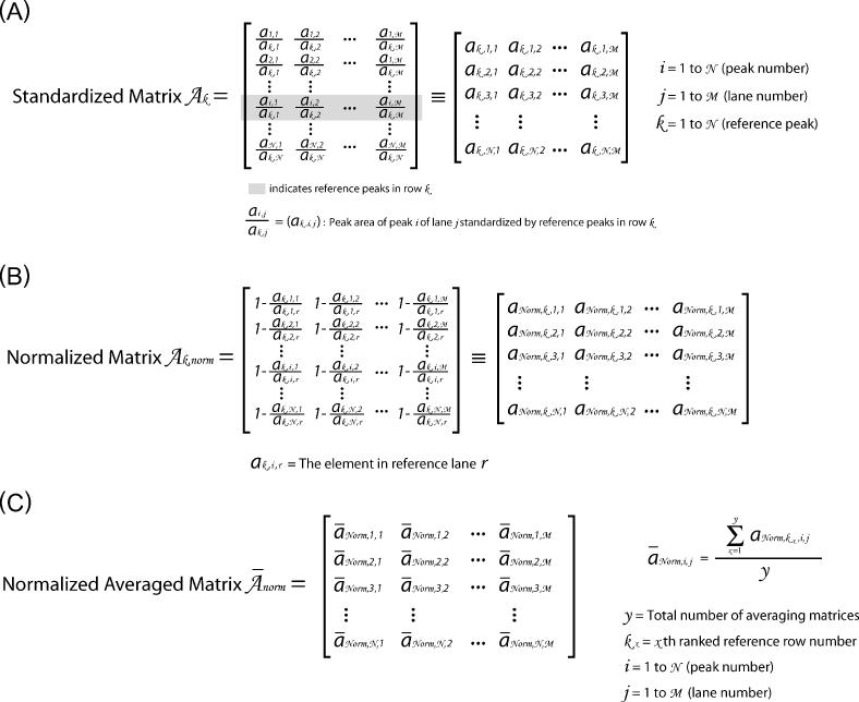
An outline of the transformation of the ‘standardized’ data to ‘relative protection’ values that range from zero to one where one denotes complete protection and negative numbers denote enhancements in •OH reactivity. (A) The standardized matrices A_k are ranked based on the quality calculation described in the text. (B) Each element in matrices A_k is divided by the element in the reference lane (in same row) and then subtracted from 1. (C) The top-ranked standardized matrices (typically five) are averaged to generate the normalized averaged matrix (Ā_norm) that is then plotted for inspection or subject to further analysis.

Data visualization

The peak-fitting approach to the quantitative analysis of footprinting experiments yields a plethora of titration data potentially encompassing tens to hundreds of nucleotides. In contrast to generating tens to hundreds of titration curves, we have found it useful to display the entire dataset as a false-color, two-dimensional map (often referred to as ‘thermograms’) that permits easy visualization of the changes in hydroxyl radical reactivity (22). Manipulation of the color-mapping palette and arithmetic interpolation of the peak area data enhances visualization of the transitions. From this complete representation of the data, the nucleotide or nucleotides whose transition is to be further analyzed can be chosen. Since a standard implementation of commercial software has been used to generate color maps (KyPlot v2 by Koichi Yoshioka), it will not be further described.

RESULTS

Generation of a line profile

Storage phosphor imaging of footprinting gels virtually eliminates the need to correct for background density and provides enhanced dynamic range when sufficient radioactivity and/or exposure time takes advantage of the 16 bit density sampling. Drawing ‘line profiles’ down lanes and averaging across the middle 50% is computationally efficient [compared with separating, analyzing then averaging a series of single pixel wide lines (12)], and minimizes error due to the broadening or narrowing characteristics of the ends of the electrophoretic bands. In the absence of a significant skew, bending or smiling in the band shapes, this approach generates good peak shapes that can be well fit by the Lorentzian peak function. We note that automation of the generation of line profiles would accelerate the analysis of footprinting gels and that such operations are included in some contemporary software packages.

Peak fitting

The accuracy and precision of a peak-fitting operation is critically dependent upon both the constraints used in the analysis and the attentiveness of the investigator conducting the analysis. The Lorentzian function has been shown to provide the best description of an electrophoretic band line profile (12) and will be used in our analyses. The Lorentzian function (Equation 1) has two parameters that affect the peak area, w_n and A_n (Equation 2), whose correlation is a key consideration when fitting a line profile due to overlap of the electrophoretic bands. This correlation can be limited experimentally by higher resolution electrophoretic separation and/or limiting the number of bands being analyzed, or, computationally, by setting constraints during peak fitting as described below.

For example, peak fitting a line profile without constraints (other than a fixed baseline) can leads to the results that are grossly in error (Figure 4A, arrow). Such a misfit peak will dominate and thus invalidate a fit. This pitfall can be circumvented by considering that the electrophoretic mobility of bands is a function of fragment length (data not shown). The broadening of bands are also a function of their distance of electrophoretic migration (29,30). Thus, the widths of neighboring bands are empirically calculated as the function of inter-peak distance and peak number (the latter roughly proportional to the logarithm of electrophoretic mobility). That this relationship holds true is seen by the ratio of peak width to average inter-peak distance [w/(xc_n+1 − xc_n), w/(xc_n − xc_n−1)] linearly increasing with the distance a peak travels down the gel (Figure 4B).

Figure 4.

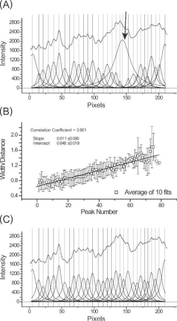
An overview of constrained peak fitting. (A) Shown are the results of an unconstrained peak-fitting session in which uniform peak widths were initially assigned. Note the variability of the peak widths far beyond the physically appropriate value in particular, the peak highlighted by the arrow. (B) The results of a calibration carried out using Equation 6 showing the linear relationship between peak number and peak width/inter-peak distances (). (C) The improvement resulting from the application of Equation 6 together with the peak width constraints that are described in the text. While correlation coefficients for panels A and C are 0.99981 and 0.99967, respectively, panel C accurately reflects the properties of the electrophoretic band separation.

This relationship is implemented in the ‘peak width assignment’ routine [Peak Fitting step (ii)] by

where P_n is the target peak number, w_n is peak width to be calculated for P_n, is the average inter-peak distance at peak P_n, m is the slope and b the intercept. is calculated automatically by the distance of peak P₂ from adjacent P₁ and P₃, P₃ from adjacent P₂ and P₄, etc., and used for the calculation of each peak width w_n. The coefficients m = 0.65 and b = 0.011 were empirically determined from the linear fit of the data of Figure 4B. (These coefficients need to be determined for a particular gel electrophoresis protocol since the inter-peak distance and the dispersion of the bands may be dependent of the particular gel system being used.) Equation 6 and the empirically determined coefficients are then used to assign initial values of w_n for any set of peaks derived from electrophoretograms obtained using the calibrated gel system.

Figure 5 demonstrates the value of this procedure on a lane profile that was difficult to fit due to changes in peak widths down the lane. Panels A and B compare results obtained without assigning the peak width as described in step (ii) while panel B shows the results obtained following peak width assignment. The improved residuals of panel B show that the process significantly improves the quality of the fitted peaks. The absence of systematic error in the fitted peaks highlights the consistency of electrophoretic data with the simple linear model for peak width.

Figure 5.

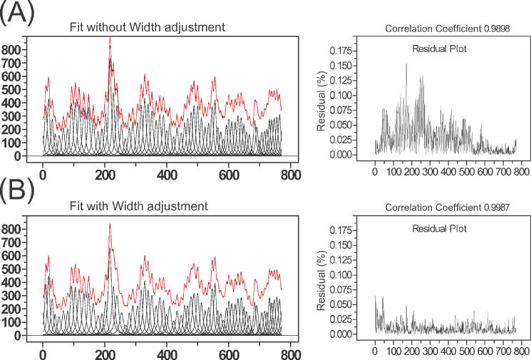
(A) The left panel shows the results obtained following fitting without peak width assignment prior to the chi-square minimization routine. The initial peak widths are uniform and the peak width boundaries are constrained to ±15% of initial value. The residual plot (right panel) shows substantial error. Since the peak width was not adjusted prior to minimization, some peak widths that reached the boundaries could not converge to their minimum and are thus trapped at values that are narrower or wider than they should be. (B) The left panel shows the results obtained following assignment of the initial peak widths using Equation 6 followed by adjustments as described in the text using the same fitting conditions as in (A). The significant improvement in the residuals is seen in the right panel. Since the peak widths are assigned prior to chi-square minimization routine, the values can be optimized within the 15% of boundaries.

Peak fitting step (iii) further refines the initial peak parameters prior to the full fitting of the data through an iterative refinement of the peak width model implemented by Equation 6 in step (ii) in order to guarantee that a global minimum can be achieved within the constraints.

Peak fitting step (iv) is the nonlinear least-squares minimization of the lane profile to Equation 1. If well-separated peaks characterize the lane profile, constraints on the fitted parameters (xc_n, A_n and w_n) are not required and the fit is iterated until the correlation coefficient ceases to increase. However, since it is desirable to extract as much information from electrophoretograms as possible, investigators will (and indeed should) always try to ‘push the limit’ of resolution of their analysis. In such cases, physically meaningless fits such as those shown in Figure 4A may result. We have empirically determined that such excursions of individual values of w_n can be prevented by serial fits in which w_n is constrained within 15% initially (in order to generate a ‘template’) and 5% for the subsequent analyses of the other lanes in the transition (data not shown). The 15% tolerance is necessary to accommodate the deviations in w_n predicted from Equation 6. Iterating until the correlation coefficient cease to decrease (<0.0005%) typically yields overall correlation coefficients of 0.999 to 0.9999 for average quality electrophoretograms.

When a series of replicates, a titration or a time course have been generated, each lane of an experiment must be fit using the same protocol and constraints. It is advantageous with regard to accuracy, precision and efficiency to utilize the results of the initial fit as a template for the analysis of subsequent lanes. This use of a template takes advantage of the incremental nature of the analysis of a transition since typically there are only incremental differences of peak intensity between sequential lanes of an isotherm or time course. In particular, accurate and precise quantitation of ‘protected’ peaks whose amplitudes will be small is enhanced by the determination of xc_n for lanes where the amplitude of these peaks is large.

Standardization/normalization

The choice of the peak(s) to be used as a standard is critical to the accuracy of the resolved transition. The key characteristic of a good standard is that it does not systematically change over the course of the transition being analyzed. The impact of standardization can be readily seen in the protection patterns calculated for the Mg²⁺-mediated folding of RNA (Figure 6A); different standard peaks yield different footprinting patterns. A bad standard can yield either meaningless or, worse, misleading results.

Figure 6.

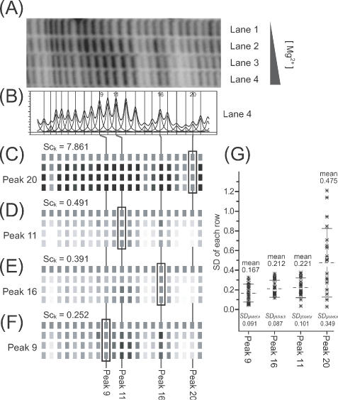
(A) A section of a gel image of a titration of the Tetrahymena ribozyme with increasing concentrations of Mg²⁺ to induce folding. Bands protected from ·OH cleavage as the concentration of Mg²⁺ increases (bands 2, 14–15, 18–20) are readily recognizable. (B) The band density profile and fitted peaks obtained for lane 4. (C–F) Reconstructions of gel images generated from ‘standardized’ and ‘normalized’ data derived from the gel image of (A) using the indicated peak as the standard. (G) The distribution of standard deviation values of each row (residues 1–21 in the profile), their mean values and SD_global,k values.

Choosing a standard row in the case of sequence-specific protein binding to a well characterized set of a few nucleotides within the gel is often trivial, while making the best choice is often not obvious in the case of complex transitions such as those typically observed for the folding of large RNA molecules. Indeed, even for the ‘trivial’ case cited above, long-range interactions or conformational changes propagated along the DNA might make choosing the appropriate standard non-trivial. Thus, even for simple systems it is desirable to have an unbiased selection of standard peaks.

The method that we have developed for automated standard selection is implemented through the calculation of the ‘score’, Sc_k (Equation 4). While SD_global,k values reflect the variance within a column of the matrix ν_norm,i,k, this parameter does not provide information about the magnitude of the values. Including the term 〈SD_norm,k〉² in the score calculation (Equation 4) allows consistent comparisons among the scores to be made since the area of the peak does not bias the ranking of peaks as standards.

Figure 6 shows the calculation of footprint titration protection patterns utilizing each of the four different standard peaks. The results of these calculations demonstrates that SD_global,k and its corresponding mean value is a less accurate measure of standard peak quality than the score, Sc_k. Panel A shows the electrophoretogram of an RNA folding titration as a function of increasing [MgCl₂] in with regions of •OH protection clearly evident at high [MgCl₂]. This example was chosen because the changes in •OH reactivity are visible in the electrophoretogram allowing direct comparison with the •OH reactivity profiles reconstructed from the standardized peak areas. Panel B is a line profile for lane 4 and its fitted peaks.

Peak 20 is obviously a poor standard since its •OH reactivity titrates with [MgCl₂] (panel A). This is evident by comparing panels C and A; the calculated •OH reactivity pattern does not match the electrophoretogram. The measures SD_global,k and Sc_k both reflect the poor quality of this peak as a standard. Peak 11 is clearly a better standard than peak 20 by the numerical as well as visual criteria (panel D). While peaks 16 and 9 are both better standards than peak 11, differences between SD_global,k and Sc_k as quality evaluators can be discerned (Panels E & F). While SD_global,k is slightly smaller for peak 16 compared to peak 9, its mean value is greater, reflecting a greater systematic deviation. In contrast, Sc_k is lowest for peak 9, reflecting the absence of systematic error in the data standardized using this peak. Figure 7 illustrates this relationship by viewing the distribution of peak area values within the individual electrophoretic lanes (Figure 6A). The values of the ‘good’ standard peak 9 cluster around the median value reflecting their random distribution. In contrast, the broad asymmetric distribution of the values of peak 20 illustrates that it is a very poor standard.

Figure 7.

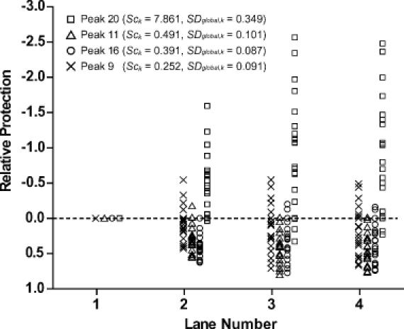
The distribution of relative protection values after standardization by different reference peaks. The relative protection values of the peaks in the lanes are plotted for each lane after standardization. The systematic deviations can be easily seen for the data standardized by inappropriate reference bands. The data standardized by peak 20 show significant deviations toward the enhancement while the data standardized by peak 11 show opposite, indicating protection in peak 20 and enhancement in peak 11. The difference between the data standardized by peak 16 and 9 are not as obvious as the others in Figure 6E and F (and SD_global) but the systematic deviation from the center can be seen clearly for the data standardized by peak 16. The standardization by peak 9 is clearly optimal.

Sensitivity to noise in the data

A series of simulations were performed on a model footprinting reactivity titration to test the effect of noise on the resolution of peak area values. Random noise of 5, 10 and 20% was introduced to the simulated peak area matrix (Figure 8A, top to bottom). Experimental data typically yields overall errors of 5–10%. With 10% noise, the original reactivity pattern can be easily recognized including subtle reactivity changes such as those seen at positions 18–19. Although the original reactivity pattern is recognizable with 20% noise, artifacts are now evident and subtle reactivity changes are no longer recognizable. As discussed above, 5% variance in peak width results in up to 10% variance in peak area. Therefore, peak width variance should be kept within 5% from template parameters when analyzing subtle changes in the reactivity.

Figure 8.

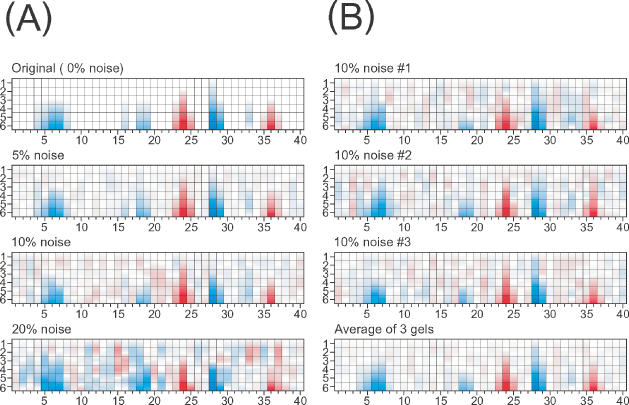
(A) The top panel is a simulated ‘perfect’ footprint pattern. The lower panels have increasing amounts of random error introduced into the simulated peak area matrices demonstrating the degradation of standardization when ≥10% noise is present in the data. (B) However, data quality can be improved by averaging multiple gels. The top three panes represent simulations into which the 10% noise was independently introduced. The bottom panel shows that averaging these three simulations recovers the simulated protection pattern at a level of 5% error.

A straightforward way to circumvent the limitations of noise on resolution of footprint reactivity patterns is to average the data from multiple gels. This will reduce statistical (so-called ‘white’) noise in the data, but will not reduce systematic errors. The white noise error reduction is , where N is the number of gels averaged. Figure 8B shows three simulated gels derived from the same original (Figure 8A, top) into which 10% error was independently introduced. Averaging of the gels (Figure 8B, bottom) reduces the apparent error in the averaged composite. This type of error reduction can be experimentally implemented in two ways. The first way is for complete transitions to be determined experimentally two or more times independently. Alternatively, replicates of each abscissa value being analyzed can be done within a single experiment. Whether, such additional measurements are necessary depends upon the overall quality of the data as well as the subtlety of reactivity changes being probed.

Following RNA folding nucleotide by nucleotide

The protocol described in this paper was developed in order to study the folding of a large RNA molecule, the T.thermophila group I intron ribozyme (22). Manual methods proved impractical for the analysis of the hydroxyl radical reactivity of each of the almost 400 nucleotides of this RNA as a function of salt concentration. The P4–P6 domain of the RNA was equilibrated in the presence of various concentrations of Na⁺ and the hydroxyl radical reactivity determined (Figure 9). A lane of ribozyme equilibrated with Mg²⁺ (the native catalytically active conformation) is included as a reference (Figure 9A, Mg²⁺ lanes and; Figure 9B, lower panel). A characteristic of Na⁺ titrations of the Tetrahymena ribozyme is the subtlety of hydroxyl reactivity changes, typically 20–50% of the difference between unfolded and folded RNA. These subtle transitions can be readily discerned on the false-color representation of the peak-fitting results (Figure 9B). Since each and every band on the gel was analyzed, a completely objective picture of the folding transition was obtained (22). Inspection and interpretation of these and related data have yielded new insights into RNA folding including revealing the presence of misfolded intermediates whose stability is transient with increasing ion concentration (22).

DISCUSSION

A robust approach for the nucleotide-by-nucleotide analysis of footprinting transition curves has been developed that allows large amounts of data to be accurately processed. Automated multiple peak-fitting procedures are more easily accomplished when absolute band assignments are available, such as in calibrated spectroscopy measurements (31), that are absent in footprint autoradiograms. Three distinct elements contribute to this approach to footprint titration analysis. First, the linear relationship between peak position (a function of electrophoretic mobility) and peak width is utilized to create initial parameter values and reduce the computation time. The constraints created reduce the probability that the fit will be trapped in a local minimum during the chi-square minimization.

Second, since a transition curve incrementally changes over its course, the results of fitting the first lane are used as ‘template’ for fitting the second lane and so on. In addition to minimizing trapping in local minima, use of a template reduces the analysis time considerably as the template sets all peak parameters at once, eliminating time-consuming peak parameter adjustment. Fitting sequential lanes is virtually a ‘single-click’ process using the template with high-quality gels.

Third, standardization of the transition curve [a procedure that corrects for uneven loading of sample onto a gel (3)] is automatically and objectively accomplished without user intervention. This feature of the protocols is perhaps the most important advancement in the analysis of complex footprint patterns. The approach used to identify ‘good standards’, i.e. identify peaks that do not change its relative intensity across the transition being probed, assumes that peaks whose •OH reactivity either decreases or increases do not heavily dominate the population. In the case of a large RNA molecule the variety of structural elements provides a wide range of •OH reactivity and thus, there is no serious problem of dominant protections/enhancements biasing the standardization result. For an analysis of protein–DNA interactions, the use of sufficiently long DNA molecules provides the appropriate context. Although this limitation has not been reached in our analyses of experimental data, investigators should remain aware and carefully compare their results for other relevant biological information.

SUPPLEMENTARY MATERIAL

Supplementary Material is available at NAR Online.

Supplementary Material is available at NAR Online.

REFERENCES

- 1.Takamoto K. and Chance,M. (2004) Footprinting methods to examine the structure and dynamics of nucleic acids. In Myers,R.A. (ed.), Encyclopedia of Molecular Cell Biology and Molecular Medicine, 2nd edn. Wiley VCH, Weinheim, Germany, pp. 569–578. [Google Scholar]
- 2.Petri V. and Brenowitz,M. (1997) Quantitative nucleic acids footprinting: thermodynamic and kinetic approaches. Curr. Opin. Biotechnol., 8, 36–44. [DOI] [PubMed] [Google Scholar]
- 3.Brenowitz M., Senear,D.F., Shea,M.A. and Ackers,G.K. (1986) ‘Footprint’ titrations yield valid thermodynamic isotherms. Proc. Natl Acad. Sci. USA, 83, 8462–8466. [DOI] [PMC free article] [PubMed] [Google Scholar]
- 4.Brenowitz M., Senear,D.F., Shea,M.A. and Ackers,G.K. (1986) Quantitative DNase footprint titration: a method for studying protein–DNA interactions. Methods Enzymol., 130, 132–181. [DOI] [PubMed] [Google Scholar]
- 5.Tullius T.D. and Dombroski,B.A. (1985) Iron(II) EDTA used to measure the helical twist along any DNA molecule. Science, 230, 679–681. [DOI] [PubMed] [Google Scholar]
- 6.Tullius T.D. and Dombroski,B.A. (1986) Hydroxyl radical ‘footprinting’: high-resolution information about DNA–protein contacts and application to lambda repressor and Cro protein. Proc. Natl Acad. Sci. USA, 83, 5469–5473. [DOI] [PMC free article] [PubMed] [Google Scholar]
- 7.Celander D.W. and Cech,T.R. (1991) Visualizing the higher order folding of a catalytic RNA molecule. Science, 251, 401–407. [DOI] [PubMed] [Google Scholar]
- 8.Latham J.A. and Cech,T.R. (1989) Defining the inside and outside of a catalytic RNA molecule. Science, 245, 276–282. [DOI] [PubMed] [Google Scholar]
- 9.Aydogan B., Marshall,D.T., Swarts,S.G., Turner,J.E., Boone,A.J., Richards,N.G. and Bolch,W.E. (2002) Site-specific OH attack to the sugar moiety of DNA: a comparison of experimental data and computational simulation. Radiat. Res., 157, 38–44. [DOI] [PubMed] [Google Scholar]
- 10.Balasubramanian B., Pogozelski,W.K. and Tullius,T.D. (1998) DNA strand breaking by the hydroxyl radical is governed by the accessible surface areas of the hydrogen atoms of the DNA backbone. Proc. Natl Acad. Sci. USA, 95, 9738–9743. [DOI] [PMC free article] [PubMed] [Google Scholar]
- 11.Strahs D. and Brenowitz,M. (1994) DNA conformational changes associated with the cooperative binding of cI-repressor of bacteriophage lambda to OR. J. Mol. Biol., 244, 494–510. [DOI] [PubMed] [Google Scholar]
- 12.Shadle S.E., Allen,D.F., Guo,H., Pogozelski,W.K., Bashkin,J.S. and Tullius,T.D. (1997) Quantitative analysis of electrophoresis data: novel curve fitting methodology and its application to the determination of a protein–DNA binding constant. Nucleic Acids Res., 25, 850–860. [DOI] [PMC free article] [PubMed] [Google Scholar]
- 13.Smith J. and Singh,M. (1996) System for accurate one-dimensional gel analysis including high-resolution quantitative footprinting. Biotechniques, 20, 1082–1087. [DOI] [PubMed] [Google Scholar]
- 14.Pastor N., Weinstein,H., Jamison,E. and Brenowitz,M. (2000) A detailed interpretation of OH radical footprints in a TBP–DNA complex reveals the role of dynamics in the mechanism of sequence-specific binding. J. Mol. Biol., 304, 55–68. [DOI] [PubMed] [Google Scholar]
- 15.Sclavi B., Sullivan,M., Chance,M.R., Brenowitz,M. and Woodson,S.A. (1998) RNA folding at millisecond intervals by synchrotron hydroxyl radical footprinting. Science, 279, 1940–1943. [DOI] [PubMed] [Google Scholar]
- 16.Sclavi B., Woodson,S., Sullivan,M., Chance,M. and Brenowitz,M. (1998) Following the folding of RNA with time-resolved synchrotron X-ray footprinting. Methods Enzymol., 295, 379–402. [DOI] [PubMed] [Google Scholar]
- 17.Sclavi B., Woodson,S., Sullivan,M., Chance,M.R. and Brenowitz,M. (1997) Time-resolved synchrotron X-ray ‘footprinting’, a new approach to the study of nucleic acid structure and function: application to protein–DNA interactions and RNA folding. J. Mol. Biol., 266, 144–159. [DOI] [PubMed] [Google Scholar]
- 18.Dhavan G.M., Crothers,D.M., Chance,M.R. and Brenowitz,M. (2002) Concerted binding and bending of DNA by Escherichia coli integration host factor. J. Mol. Biol., 315, 1027–1037. [DOI] [PubMed] [Google Scholar]
- 19.King P.A., Jamison,E., Strahs,D., Anderson,V.E. and Brenowitz,M. (1993) ‘Footprinting’ proteins on DNA with peroxonitrous acid. Nucleic Acids Res., 21, 2473–2478. [DOI] [PMC free article] [PubMed] [Google Scholar]
- 20.Swisher J.F., Su,L.J., Brenowitz,M., Anderson,V.E. and Pyle,A.M. (2002) Productive Folding to the native state by a Group II intron ribozyme. J. Mol. Biol., 315, 297–310. [DOI] [PubMed] [Google Scholar]
- 21.Chaulk S.G. and MacMillan,A.M. (2000) Characterization of the Tetrahymena ribozyme folding pathway using the kinetic footprinting reagent peroxynitrous acid. Biochemistry, 39, 2–8. [DOI] [PubMed] [Google Scholar]
- 22.Takamoto K., He,Q., Morris,S., Chance,M.R. and Brenowitz,M. (2002) Monovalent cations mediate formation of native tertiary structure of the Tetrahymena thermophila ribozyme. Nature Struct. Biol., 9, 928–933. [DOI] [PubMed] [Google Scholar]
- 23.Uchida T., He,Q., Ralston,C.Y., Brenowitz,M. and Chance,M.R. (2002) Linkage of monovalent and divalent ion binding in the folding of the P4–P6 domain of the Tetrahymena thermophila ribozyme. Biochemistry, 41, 5799–5806. [DOI] [PubMed] [Google Scholar]
- 24.Dixon W.J., Hayes,J.J., Levin,J.R., Weidner,M.F., Dombroski,B.A. and Tullius,T.D. (1991) Hydroxyl radical footprinting. Methods Enzymol., 208, 380–413. [DOI] [PubMed] [Google Scholar]
- 25.Tullius T.D. (1988) DNA footprinting with hydroxyl radical. Nature, 332, 663–664. [DOI] [PubMed] [Google Scholar]
- 26.Ralston C.Y., Sclavi,B., Sullivan,M., Deras,M.L., Woodson,S.A., Chance,M.R. and Brenowitz,M. (2000) Time-resolved synchrotron X-ray footprinting and its application to RNA folding. Methods Enzymol., 317, 353–368. [DOI] [PubMed] [Google Scholar]
- 27.Celander D.W. and Cech,T.R. (1990) Iron(II)-ethylenediaminetetraacetic acid catalyzed cleavage of RNA and DNA oligonucleotides: similar reactivity toward single- and double-stranded forms. Biochemistry, 29, 1355–1361. [DOI] [PubMed] [Google Scholar]
- 28.Di Marco V.B. and Giorgio Bombi,G. (2001) Mathematical functions for the representation of chromatographic peaks. J. Chromatgr. A, 931, 1–30. [DOI] [PubMed] [Google Scholar]
- 29.Brahmasandra S.N., Burke,D.T., Mastrangelo,C.H. and Burns,M.A. (2001) Mobility, diffusion and dispersion of single-stranded DNA in sequencing gels. Electrophoresis, 22, 1046–1062. [DOI] [PubMed] [Google Scholar]
- 30.Meistermann L. and Tinland,B. (1998) Band broadening in gel electrophoresis of DNA: measurements of longitudinal and transverse dispersion coefficients. Phys. Rev. E, 58, 4801–4806. [Google Scholar]
- 31.Marinkovic N.S., Huang,R., Bromberg,P., Sullivan,M., Sperber,E., Moshe,S., Miller,L.M., Jones,K., Chouparova,E., Franzen,S. et al. (2002) Center for Synchrotron Biosciences' U2B Beamline: an international resource for biological infrared spectroscopy. J. Synchrotron Radiat., 9, 189–197. [DOI] [PubMed] [Google Scholar]