Phase-Locked Loop for Precisely Timed Acoustic Stimulation during Sleep

Abstract

Background

A Brain-Computer Interface could potentially enhance the various benefits of sleep.

New Method

We describe a strategy for enhancing slow-wave sleep (SWS) by stimulating the sleeping brain with periodic acoustic stimuli that produce resonance in the form of enhanced slow-wave activity in the electroencephalogram (EEG). The system delivers each acoustic stimulus at a particular phase of an electrophysiological rhythm using a Phase-Locked Loop (PLL).

Results

The PLL is computationally economical and well suited to follow and predict the temporal behavior of the EEG during slow-wave sleep.

Comparison with Existing Methods

Acoustic stimulation methods may be able to enhance SWS without the risks inherent in electrical stimulation or pharmacological methods. The PLL method differs from other acoustic stimulation methods that are based on detecting a single slow wave rather than modeling slow-wave activity over an extended period of time.

Conclusions

By providing real-time estimates of the phase of ongoing EEG oscillations, the PLL can rapidly adjust to physiological changes, thus opening up new possibilities to study brain dynamics during sleep. Future application of these methods hold promise for enhancing sleep quality and associated daytime behavior and improving physiologic function.

1 Introduction

Slow-wave sleep (SWS) is a very distinctive feature of sleep in mammals and birds [1]. SWS has a restorative role and it has many physiological and behavioral implications. Many studies have established that SWS is associated with the stabilization of memories for long-term storage [2]. SWS diminishes with age, both in duration and intensity, and this decline correlates with memory changes from before and after sleep and with impairments in cognitive performance [3]. In addition, analyses of sleep in individuals with amnestic mild cognitive impairment (aMCI) showed reduced slow-wave activity (SWA), the physiologic measurement of SWS, compared to age-matched controls [4]. Experimental suppression of SWS also impairs metabolic function, and SWS is thought to play an important role in the regulation of cardiometabolic function [5]. Another important function of SWS is the production and regulation of hormones, with an important example being the growth hormone [6]. Recently it has been demonstrated that SWS may play a role in flushing toxins from the brain, particularly β-amyloid [7]. Thus, enhancing SWS could have many beneficial implications for cognitive and physical health.

Given the role of sleep in declarative memory consolidation [8, 9], there has been great interest to enhance SWS. One such method is to pass slow oscillatory electrical activity into the brain transcranially to modulate neuronal excitability during sleep so as to increase endogenous SWA and improve consolidation. In two studies [10, 11], healthy young people learned lists of word pairs before going to sleep. In tests given both before and after sleep, subjects attempted to recall the second word of each pair in response to the first. Remarkably, the results showed that this method of Low-Frequency Stimulation (LFS) during sleep increased SWA and improved memory. Recall was better if the retention interval included LFS compared to sham stimulation during sleep.

Although LFS can increase SWA, it has practical and technical limitations. From a technical standpoint, it is difficult to record EEG activity during the stimulation because of the artifacts created by the applied electrical field. Given that these sorts of stimulation methods can generate complicated patterns of activated and deactivated brain areas [12], it can be difficult to specify how the electrical stimulus influences neuronal activity. LFS is also impractical for regular use because it requires the assistance of trained technicians. Finally, while the intensity of the electrical stimulation is relatively low and likely safe in the short-term, long-term studies of efficacy and safety are lacking [13].

An innovative method to enhance slow waves is to use acoustic stimulation. It is well established that auditory tones can influence EEG activity by producing K-complexes, which are similar in structure and are precursors to slow-waves [14]. Tononi and colleagues showed that auditory stimulation during sleep can enhance SWA in young adults [15]. The tones were of short duration (50 ms) and were applied using a fixed intra-tone interval (ITI) of 1 Hz. In this protocol, stimulation was delivered in a sequence of 15 consecutive tones (block ON), followed by periods when tones were not played (block OFF) [15]. The block on/off sequence was adopted to track the effect of the auditory stimulation on SWA at regular intervals during deep sleep and also to tap into hypothesized infraslow oscillations in non-rapid eye movement (NREM) sleep that seem to occur about every 15 seconds [16].

The method of fixed ITI acoustic stimulation was also shown to enhance slow waves by another research group [17]. Stimulation at 0.8 Hz beginning prior to sleep delayed sleep onset and enhanced SWA. Further stimulation studies showed that the response can change as a function of the timing of the stimulus relative to the phase of the slow EEG rhythms [18-20]. These results may reflect the up and down phases of slow-wave oscillations, which correspond to periods of neuronal activity and quiescence [21]. Therefore, the ability to synchronize auditory stimulation to a particular phase of the slow wave could lead to more consistent enhancement of slow waves.

To take into consideration these phase-dependent responses to stimulation, we adopted a more complex stimulation approach. Ngo and colleagues [22] introduced a method that allows the auditory stimulation to be approximately tuned to the phase of the slow wave. Their results showed that this phase-dependent auditory stimulation can increase slow oscillations as well as phase-coupled spindle activity. In addition, they showed that stimulation to enhance slow waves leads to improved declarative memory performance. Presumably the enhancement of SWA is beneficial because it is conducive to neuronal synchronization, and because spindle activity reflects an essential aspect of memory consolidation [23]. Furthermore, phase-dependent stimulation could also be tuned to the down state, in which case it did not enhance SWA and did not have an effect on memory [22].

In this paper, we describe the reasoning behind using a methodology with a phase-locked loop (PLL) to improve sleep. This work demonstrates that the PLL is a superior algorithm to track a signal, such as in modeling EEG slow waves, and identify a target phase for real time application, such as with delivery of stimuli a particular slow-wave phase. Phase targeting is important because different slow-wave phases correspond to different physiological states that directly influence neural activity, and stimulation at different phases can produce different effects. We include some physiological results but do not include a complete investigation of the effectiveness of the method in enhancing slow-wave sleep in a group of participants. Rather, we provide here a comprehensive methodological analysis that focuses on the phase-tracking ability of the PLL. It remains to show how the method compares with other methods and how effective and reliable it is for individuals with normal sleep patterns or with abnormal sleep patterns, as in older individuals. Ong and colleagues [24] have described an initial application of this method to study sleep in a group of young participants.

2 Material and Methods

2.1 Phase-Locked Loop

2.1.1 PLL Theory

We have independently developed a new method for phase-tracking auditory stimulation that consists of an adaptive feedback algorithm based on a PLL that tracks the phase of the underlying EEG and delivers tones at a particular preferential phase [25]. This stimulation method is more general (it can be applied easily to any particular target phase), flexible (it adapts automatically to the slow wave individual characteristics), accurate and precise (it targets the right phase much better and more consistently) than the slow-wave detection procedure described by Ngo and colleagues or the more recent one described by Cox and colleagues [26].

A PLL is a control system that generates an output signal whose phase is related to the phase of an input reference signal. When it is implemented as an electronic circuit it typically consists of a variable frequency oscillator and a phase detector. This circuit compares the phase of the input signal with the phase of the signal derived from its output oscillator and adjusts the frequency of its oscillator to keep the phases matched. The signal from the phase detector is used to control the oscillator in a feedback loop.

Because frequency is the time derivative of phase, keeping the input and output phase in lock step implies keeping the input and output frequencies in lock step. Consequently, a phase-locked loop can track an input frequency, or it can generate a frequency that is a multiple of the input frequency. The former property is used for demodulation [27], and the latter property is used for indirect frequency synthesis [28].

Phase-locked loops are widely employed in radio, telecommunications, computers, and other electronic applications [29]. They can be used to recover a signal from a noisy communication channel, generate stable frequencies at a multiple of an input frequency, or distribute clock timing pulses in digital logic designs such as microprocessors. The PLL can also be implemented in a purely software realization.

There are many proposals in the literature for using the PLL in biomedical applications, as for example to model interactions of biochemical reactions [30], to analyze circadian rhythms [31, 32], to describe motor control [33], and to design Brain-Computer Interfaces [34]. PLL processes may reflect the activity of brain structures in charge of the processing of sensory-motor information [35]. The PLL has been implemented in real time to analyze and classify EEG oscillations in the alpha, beta, delta, and theta bands [27, 36-38]. The PLL has been also utilized to detect particular features of the EEG such as spindles [39].

Our particular application of the PLL for the induction of SWA is designed to rhythmically deliver an acoustic tone in a given range around the target frequency of 1 Hz and phase-locked with endogenous slow-wave oscillations. Our preliminary results indicate that synchronizing the stimulation with the phase of the EEG dramatically increases the efficacy and characteristics of the slow-wave induction in comparison with a fixed interval stimulation. Here we describe the performance and the applicability of a PLL for following and guiding a stimulation protocol that has a flexible but limited range of frequencies and that is phase-locked with the quasi-periodic fluctuations of the EEG during SWS.

2.1.2 PLL design

There is a vast body of literature describing the details of a PLL and its implementation, which we summarize briefly here. A PLL has three main components: 1) Phase Detector (PD), 2) The Loop Filter (LF), and 3) Voltage Controlled Oscillator (VCO). See fig. 1 for a diagram of the PLL algorithm.

Fig 1.

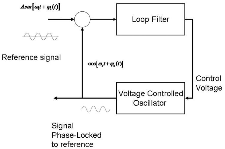
Schematic of the PLL loop. An input sinusoidal signal (the sleep-wave oscillations) with given phase is multiplied by a computer generated signal that is shifted by 90 degrees with the input signal. A low pass filter selects the difference of the phases of these two signals if the phase difference is small (the PLL is nearly locked). A voltage controlled oscillator (VCO) multiplies the phase difference between the two oscillators by a constant. This phase is added to the computer generated signal phase in order to match it to the reference signal.

Let s₁(t) be the input reference signal (in our case the EEG signal during SWS). We are assuming in this example that the signal is a sine wave with a given angular frequency ω (the real EEG it is actually a more complicated narrow band signal). The signal also has a non-zero phase ϕ₁(t). Let s₂(t) be another signal, also a sinusoidal function with angular frequency ω, that we want to phase lock with the reference signal. This is our PLL signal that we will use for auditory stimulation. The signal s₂(t) has an initial phase difference with s₁(t) equal to 90°. If we multiply the two signals, we have:

$$s_1=A_{1}sin[\omega t+{\varphi }_1(t)],$$ (1)

$$s_2=A_{2}sin[\omega t+{\varphi }_2(t)],$$ (2)

$$s_3(t)=s_1(t)s_2(t)=K_d{A}_{1}sin[\omega t+{\varphi }_1(t)]A_{2}sin[\omega t+{\varphi }_2(t)];$$ (3)

where K_d is the gain of the multiplier or phase detector. We can rewrite equation (3) using trigonometric identities:

$$s_3(t)=\frac{K_d{A}_1{A}_2}{2}sin[{\varphi }_2(t)-{\varphi }_1(t)]+\frac{K_d{A}_1{A}_2}{2}sin[2\omega t+{\varphi }_2(t)+{\varphi }_1(t)].$$ (4)

When rewritten in this way, the equation s₃(t) has two distinct parts one that is frequency independent and one that is a function of twice the original frequency (plus the sum of the two phases). The frequency-independent phase is a function of the phase difference ϕ₂(t)–ϕ₂(t). We can select this relevant information by applying a low-pass filter to the multiplier s₃(t) to obtain the error signal:

$$s_e=\frac{K_{\mathit{\text{LPF}}}{K}_d{A}_1{A}_2}{2}sin[{\phi }_2(t)-{\phi }_1(t)];$$ (5)

where K_LPF is the low pass filter gain.

The last component of the PLL is the VCO. The error signal gives us information about the input signal. The goal is to synchronize the output signal with input signal, so we need to minimize the error signal. We accomplish this by changing the phase of signal s₂(t) to match the phase of signal s₁(t). The VCO generates a periodic signal with a frequency that is proportional to a control signal, in our case the error signal. When the error signal is zero the VCO in a PLL produces a signal with a center frequency ω_c that is equal to the input signal. When the error signal is non-zero the VCO responds by changing its frequency. The rate of change of the frequency in the VCO represents its sensitivity K_o:

$${\omega }_{\mathit{\text{out}}}={\omega }_c+K_o{s}_e(t)={\omega }_c+{\varphi }_2(t).$$ (6)

Phase is the integral of the frequency:

$${\varphi }_i=2\pi {\int }_0^t{f}_i(t)dt$$ (7)

And applying (7) to equation (6):

$${\varphi }_2(t)=2\pi K_o{\int }_0^t{s}_e(t)dt=2\pi K_o{s}_e(t)t;$$ (8)

under the assumption of a linear error.

Then if the error signal has a non-zero amplitude, the phase of the VCO signal will keep increasing until it goes back to zero. The error signal in (5) can be rewritten as:

$$s_e(t)=\frac{K_{\mathit{\text{LPF}}}{K}_d{A}_1{A}_2}{2}sin[2\pi K_o{s}_e(t)t-{\phi }_1(t)]$$ (9)

Making the assumption that the error in phase is small, then we can simplify the above using sin(θ) ≈ θ:

$$s_e(t)=\frac{K_{\mathit{\text{LPF}}}{K}_d{A}_1{A}_2}{2}[2\pi K_o{s}_e(t)t-{\phi }_1(t)].$$ (10)

Equation (10) illustrates the corrective, iterative process of the PLL. If the error signal is non-zero the phase keeps changing linearly, but as the phase of the VCO changes, the updated difference in phase becomes smaller at the next iteration. This process continues until the error signal amplitude approaches zero and PLL is said to be phase-locked.

The PLL behaves in a manner similar to that of an adaptive band-pass filter but with a smoother response and a larger gain. The total gain is K = K_LPFK_dK_o A₂.

2.1.3 PLL control system representation

The PLL can be analyzed also as a control system using the Laplace transform. The closed-loop transfer function takes the form [27]:

$$H(s)=\frac{KF(s)}{s+KF(s)},$$ (11)

where s = iω and F(s) = (1 + sτ₂)/(1 + sτ₁) is the transfer function of the low-pass filter, in this case a lag-lead filter.

We can then rewrite the closed-loop transfer function as:

$$H(s)=\frac{K(1+s{\tau }_2)}{{\tau }_1{s}^2+(1+K{\tau }_2)s+K}.$$ (12)

The denominator of equation (12) has the form of a harmonic oscillator s² + 2ζω_ns + ω²_n where the natural frequency is ${\omega }_n=\sqrt{K/{\tau }_1}$ and the damping factor is ζ = 1/2ω_nτ₂. The bandwidth ω_h for the PLL can be calculated then by:

$${\omega }_h={\omega }_n{[(1+2{\zeta }^2+\sqrt{2+2{\zeta }^2}]}^{1/2}.$$ (13)

Another important parameter that determines a relevant time scale of the PLL is the lock-in time T_L:

$$T_L=\frac{2\pi }{{\omega }_n},$$ (14)

the time required for the lock-in process.

2.1.4 Parameter optimization

To optimize the PLL parameters, we performed simulations using a digital PLL on a segment of EEG containing SWS during naps in 5 subjects. These simulations were conducted 1) to determine the optimal parameters for sleep stage detection and PLL EEG phase tracking and targeting and 2) to demonstrate that the digital analysis could track the rhythm of slow waves and the burst-like slow-wave activity during SWS. The details of the algorithms for these functions are detailed in section 2.4.

For phase tracking and targeting, we chose the parameter values through an optimization process where we varied one parameter at the time to maximize the likelihood that the acoustic pulses would be given in a particular phase range. We chose a relatively wide bandwidth (3.7 Hz around the center frequency of 0.85 Hz) to adapt to the changes of the dominant slow-wave frequency (that can vary between 0.5 to 4 Hz). Some PLL implementations apply a band-pass filter to isolate the time evolution around a particular frequency. In our application we relied on the natural narrow-band characteristics of the EEG during SWS, so we used the raw EEG as the PLL input. The specific values that we selected for our slow-wave PLL were the following: low-pass frequency cut-off = 0.03 Hz, amplifier gain A₂ = 5, phase detector gain K_d = 6, low-pass filter gain K_LPF = 20, and VCO gain K_o = 5. The lock-in time T_L is 3.7 s. These optimal PLL parameters were similar between individuals.

2.2 Experimental design

A Matlab program for the automatic brain computer interface (BCI) was developed to control acoustic stimulation. We have tested our procedure in different age groups, both during naps and overnight. A detailed description of physiological outcomes will be presented in future papers. The goal of the present paper is to show the ability of the PLL to follow the slow-wave process and to determine the phase of the EEG online. We thus focus on results obtained during naps in young subjects.

This study was approved by the Northwestern University Institutional Review Board. We recruited 5 subjects from the community (3 males and 2 females, age range 21-25 years). Subjects underwent one stimulation nap and one sham nap separated by one week. The order of the conditions was randomly assigned. Subjects were not informed of the order of the conditions or if sounds would be played during a particular nap. Subjects wore headphones specifically designed for sleep (Acoustic Sheep Sleep Phones SP4BM) during both conditions. During the sham stimulation procedure, no sounds were played but headphones were still worn. Sound intensity ranges were determined once before the experiment and adjusted to be between a barely audible level for the subject and a level that the subject considered acceptable for during sleep. Intensity levels were adjusted during the nap session as described below.

2.3 Data acquisition

EEG data were acquired during afternoon naps from 5 subjects. Data were recorded using a Brain Products V-Amp amplifier at 500 Hz sampling frequency. High-pass hardware filtering was applied with a cutoff frequency of 0.3 Hz. We used three recording channels, one for detection of slow waves (anterior frontal channel Fpz referenced to right mastoid) and two for differential electro-oculogram (EOG), with self-adhesive, disposable, Ag/AgCl electrodes. Data were acquired in two ways: raw data at 500 Hz via the V-Amp data acquisition software and through a MatLab Application Programming Interface (API) that communicated with the V-Amp via a TCP/IP port. Every 20 ms the API sent a packet of 10 data points to the i/o MatLab function. EEG pre-processing consisted of applying a band pass filter (Chebychev second order, 0.05 dB pass-band ripple) with cut-off frequencies at 0.5 and 38 Hz to the 10 points. Data were consequently down sampled to 100 Hz to avoid aliasing. The hardware time resolution of our system is limited by the data packet delivery of the API (about 20 ms). We determined that the largest additional delay (about 40 ms) was due to the activation of the sound card (this delay can be decreased by using the MatLab Psychtoolbox and an Asio sound driver). The total measured delay was 70 ± 5 ms. As explained in Section 2.4.3, we accounted for delay by anticipating the delivery of the acoustic pulse, relative to the target phase, by a phase corresponding to the measured total delay.

Using the methods described below, the MatLab stimulation and scoring code stored downsampled EEG data, along with slow waves and spindles identified using automatic detection methods described above. In addition, data were stored to describe the online EEG scoring, the PLL output, and the timing of the auditory pulses or sham events for a total of 22 parameters. The stored data were analyzed offline using MatLab to produce the results discussed in section 3.

2.4 Algorithms

2.4.1 Sleep detection

A protocol to automatically detect sleep was implemented using the relative average power in different EEG frequency bands. Because we wanted to emphasize robustness in detecting SWS (NREM stage 3 or stage N3), we adopted a simplified classification at this step to detect a general sleep state, which corresponds roughly with early stage N2 sleep. The automatic protocol started with a default Wake stage. We used a delta root mean square (rms) continuous calculation based on the last 5 min of EEG activity to determine stage N2 sleep onset. This automatic method for detecting stage N2 sleep agreed with scoring by a human rater (detecting at least 10 min of N2) 85% of the time in average over all the subject data (standard deviation 8.5 %). We used two criteria to automatically determine when the sleep state was reached (whichever was reached first). The first criterion was for delta rms to be above an empirically determined threshold for at least 75 s. The delta rms threshold was found by collecting data from an average over 4 baseline naps without any stimulation from 4 young subjects (different from the ones used in the stimulation experiment), then calculating a histogram of delta rms for the entire data set (including waking and sleep), and then determining the delta rms value corresponding to the 40th percentile. The second criterion was the presence of spindles (total spindle duration of 1.5 s in the last 30 s) and a delta rms value equal to at least 80% of the delta rms threshold.

2.4.2 Slow wave and spindle detection

Each slow wave was detected as follows. First, a delta sleep threshold was determined as described in section 2.4.3. When delta power was above this threshold during a subsequent session, every time the EEG crossed the zero line in the negative direction a counter measured the time before the EEG trace crossed the zero line in the positive direction. The maximum negative amplitude during that time interval was also recorded. If the time interval was between 0.25-2 s (corresponding to slow-wave frequencies between 0.5 to 4 Hz) and the negative amplitude was at least 50 μV, than this event was recognized as a slow wave and its timing and characteristics were recorded. An interval of SWS was defined by detecting a minimum of 6 slow waves in a period of 30 s, which is consistent with manual scoring of SWS. This procedure identified N3 sleep stage in a very precise manner. We had an agreement of 95 % (average over 30 data sets, standard deviation 3.1 %) between our automatic detection and human expert scoring for this stage.

Spindle detection (a close variant of method discussed in [40]) consisted of the following steps applied during the baseline night. Data were filtered (Chebychev second order) at 12-16 Hz (sigma). A low-pass filter (0.5 Hz cutoff frequency) was applied to the absolute value of the output of this spindle band filter to track the slow changes over time of the spindle power. The low pass filter was applied to the last 5 seconds of data. The use of the low pass filter was necessary to recover an aproximation of the envelope (that contains the amplitude information for the spindle as an event) given that the usual Hilbert transformation used in [39] is not suitable for real-time detection. Two thresholds were determined on the basis of the distribution of power in this band. The lower and higher amplitude thresholds were 2 and 8 times the mean absolute amplitude of the filtered data. With these parameters, a spindle event was then defined as any interval when the filtered signal envelope stayed within the two thresholds for a period between 0.5 - 3 s.

2.4.3 Acoustic Stimulation

The PLL estimates EEG phase in real time (with computational delays of the order of milliseconds). As soon as a certain target phase range is reached (with a typical bandwidth of 0.3 radians), a pulse is delivered. In rare cases (less than 5%) the change in the phase is so rapid that there is a jump in phase across the target phase range. In that case, if more than a second is passed by the last pulse, a new tone is played to avoid big time gaps between consecutive stimuli.

Once the subject was determined to be asleep, the MatLab routine activated a K complex/slow-wave detection algorithm. If a K complex was detected, then brief auditory tones were played with an intertrial interval (ITI) of 5 s. The stimulus consisted of a 50-ms sequence of sine-Gaussian pulses at about 500 Hz (with 10% random variation in frequency between pulses to avoid habituation).

The auditory stimulation intensity was adjusted as follows. The maximum volume was kept below 45 dB with a minimum of 30 dB. This range was divided in 20 steps. Intensity was increased by a small step if after 4 stimuli less than 2 K-complex responses were detected within a window of 2 s after each stimulus, and decreased if an increase in alpha or beta power was observed (indicative of a possible micro-arousal) [41]. This procedure has the ability to determine individualized auditory thresholds during sleep to be used in the SWS stimulation protocol. The last intensity setting achieved in the N2 stage for each nap was the maximum used in the N3 stage. The logic behind this procedure is to find the minimal volume that can elicit K-complexes (that are considered precursors and physiological similar to slow waves) without waking up the subject.

Once the onset of the N3 stage of sleep was detected (see section 2.4.2), the SW stimulation consisted of pulses with an ITI of about 1 s. The value of the ITI was adjusted according to the phase of the slow-wave EEG through the application of the PLL. The tones were delivered when the phase of the EEG reached a certain predetermined value. This phase value could be changed online via a MatLab graphical user interface (GUI). The stimulation procedure followed an alternating pattern of blocks of n tones (block ON) and n sham tones (the times of automated tone presentation were recorded but tones were not played, block OFF). The number of tones was also a parameter the user could change at any moment during the experiment via the GUI. In the following examples, we used a phase that corresponds to the positive half-wave (just before the peak) and a sequence of 5 tones. The stimulation continued during the nap during N3 unless an arousal was detected (a sudden increase of beta or alpha power above given thresholds). The alpha and beta thresholds were calculated using the entire rms histogram for these bands from a few naps from young subjects, including all the stages, and then determining the delta rms value corresponding to the 75th percentile. Following arousal detection, a refractory time of 30 s with no stimulation began.

Although slow waves tend to occur in a narrow band (from 0.5 to 4 Hz), during sleep they appear as short bursts of activity. The PLL oscillates in a regular manner between bursts and it is able to follow the non-linear behavior of slow waves during bursts. During the bursts the PLL is locked to the EEG trace as determined by a small phase error. How well the PLL can follow the EEG depends on the parameter values, which can be adjusted to improve the performance of the PLL.

2.5 Analysis

The analyses in this work were conducted using MatLab code. We used the built in MatLab function “pwelch” to perform spectral analysis and comparison between conditions. To calculate statistical values for the phase we used the CircStat MatLab toolbox [42]. The phase for the EEG was calculated using the built in MatLab function “hilbert”. We indicated in the following sections when we performed averages among subjects and individual naps. For illustration on how the PLL outputs look like we have presented a single individual results from naps in some of the following figures. To optimize the PLL we run simulations (again using code written in MatLab) on data collected during naps changing one PLL parameter at the time (as explained in section 2.14). We also run a simulation (following as best we could the steps explained in the relevant literature) to determine the precision of the phase tracking for the Ngo et al. closed loop method [22].

3 Results

3.1 PLL phase tracking of slow wave oscillations

Fig. 2 shows EEG from channel Fpz during SWS (black curve) for one subject (subject 4). The output of the VCO is shown on the same time scale (blue curve). The PLL output closely follows the EEG trace, particularly during bursts of slow-wave activity. During these times the phase error is small and the PLL is locked. During times when the frequency characteristics of the EEG is not within the given bandwidth, the PLL oscillates in a more regular way with a sinusoidal pattern with the central frequency of the system. This feature of the PLL is useful for our purpose because our algorithm generates a tone when a certain phase range is reached for the first time. Even when a slow wave is not present, rhythmic tones are delivered in the attempt to evoke a slow wave. The tones are indicated by pink stems in Fig. 2. A first visual inspection shows that a majority of the acoustic stimuli are delivered at the target phase that in this case is between the zero crossing and the positive peak. In this example we used data from a specific nap from one subject. The statistics described in the following sections are derived from sham and stimulation naps in 5 subjects. The PLL is capable of adapting to individual sleep patterns and characteristics without the need to be further calibrated after the initial optimization using baseline information described in section 2.1.3. Whereas the method used by Cox and colleagues [26] for slow-wave phase targeting seems to perform in an inconsistent manner across different subjects, our PLL is very consistent (both within and between subjects) in how precisely the tones are delivered at a given target phase because of the inherent adaptive properties of the PLL. This section contains a detailed discussion of the phase tracking statistical performance of our algorithm.

Fig. 2.

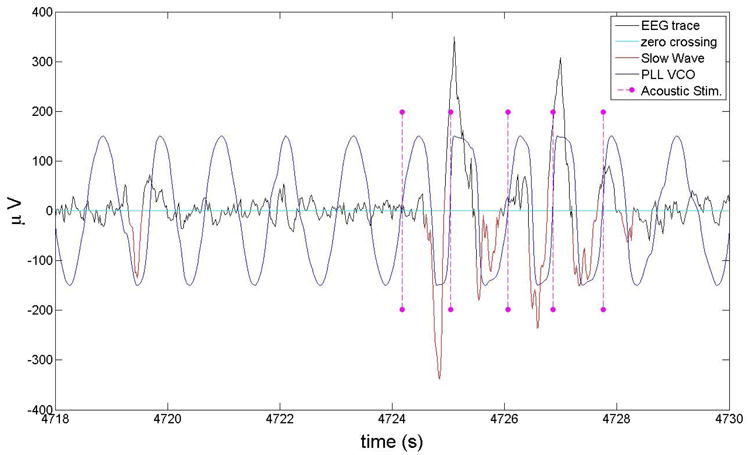
The EGG trace (subject 4) for an interval of SWS (black line), the VCO output for the PLL that matches the EEG trace (blue line), and the acoustic stimuli (pink stems). The negative half of the slow waves, as identified by our automatic code, are shown in red. Visual inspection shows that the PLL algorithm identified the right phase.

To quantify the performance of the PLL in tracking the EEG signal, we used the Hilbert transform to calculate the phase of the EEG offline. It is important to note that the PLL is designed to track the EEG activity in a narrow frequency range, so discrepancies between the PLL phase and the actual phase of the EEG can be due to the richer frequency content present in the EEG. Although the Hilbert transform is the gold standard to measure phase of a time series, it is not a useful tool to calculate the phase online because it needs to have information both about the past and the future of the time series to compute the phase at any particular point. This is the reason why we use the PLL as the online phase detector. We define the PLL Phase Error as the difference between the phase-detector output of the PLL and the phase of the EEG calculated using the Hilbert transform. Figure 3 shows the Phase Error (for subject 4) as a function of time and it is plotted superimposed on an EEG time series (to make easier the comparison of scale the EEG is divided by a factor of 10). In general, the errors become quite small in the presence of slow-wave bursts and the PLL is therefore locked to the EEG during these events. In fact, even if our sleep staging is independent from the PLL, the PLL could be used by itself to determine the presence of SWS.

Fig. 3.

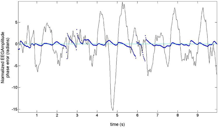
A normalized EEG trace (divided by a factor of 10, subject 4) with a superimposed Phase Error (in blue). The Phase Error is small when a burst of slow waves is present, indicating times when the PLL is locked to the EEG.

To analyze more precisely the statistical phase tracking properties of the PLL we used the circular statistic functions from the CircStat MatLab toolbox [42]. Fig. 4 top panel shows a circular histogram of the PLL Phase Error in degrees for the case of all the EEG data points in SWS that did not contain slow waves (data from all the subjects' naps). The circular histograms in the following figures have a bin size of 18 degrees each. The bottom panel of Fig. 4 is a histogram for the same quantity but for segments of data that contained slow waves (negative portion). The presence of slow waves reduced the standard deviation of the Phase Error, but introduced a small systematic error (t-test gives p=0.051); the mean value and standard deviation of the error are 12.51 ± 28.85 degrees for the no-slow-wave case and 13.63 ± 9.88 degrees for the slow-wave case (a comparison of standard deviation F-test gives a p<0.001). Fig. 5 shows the relationship between the slow-wave amplitude and the Phase Error, demonstrating that the larger the amplitude of the oscillation the smaller the error (all SWS data points from subject 4). Given that the acoustic stimulation needs to be presented at a particular phase of pre-existing slow waves oscillations it is reassuring the PLL performance is best when we observe large amplitudes (indicating the probable presence of a slow wave) and the PLL locks to the EEG.

Fig. 4.

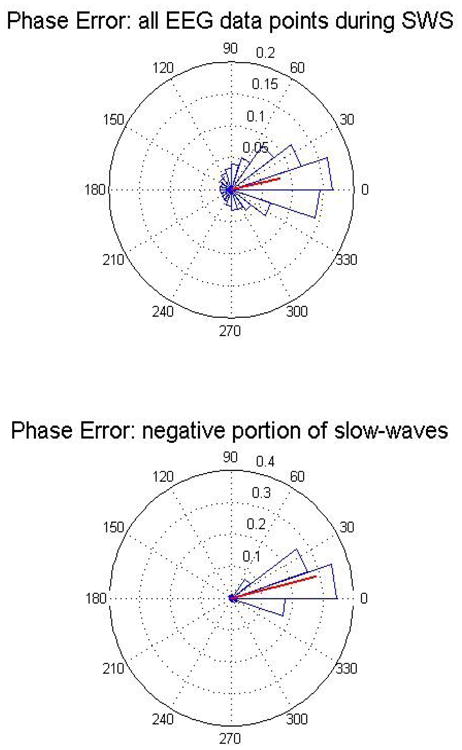
Error in phase detection (data from all the subjects' naps). The red line represents the mean phase vector. Top panel is the EEG data points during N3, bottom panel is the phase error for events that include slow waves.

Fig. 5.

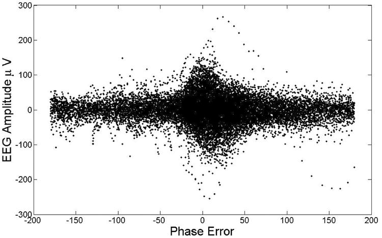
EEG amplitude versus the error in phase detection (subject 4 nap data). While for small amplitudes (less than 50 microvolts) the phase error (in degrees) is uniformly distributed for large amplitudes the phase error decreases as the amplitude increases.

3.2 Phase targeting

The interval of time in seconds between pulses is illustrated in the histogram in Fig. 6. The histogram covers a relatively large range of periods (subject 4 nap data), but with most of the pulses at a dominant period. The mean period is 1.06 seconds (0.935 Hz) and the standard deviation is 0.186 seconds (0.138 Hz).

Fig. 6.

Histogram for the time between pulses (subject 4 nap data). The mean period is 1.06 seconds (0.935 Hz) and the standard deviation is 0.186 seconds (0.138 Hz).

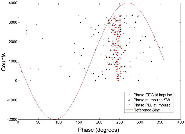
The tones are delivered when the phase detector initially reaches the target range. Fig. 7 top panel shows the phase of the EEG in degrees (as measured with the Hilbert transform, data from all naps and all the 5 subjects) at the time a tone was applied (even when a threshold-level slow wave was not detected). In this figure the down-state is at 90 degrees, the up-state is at 270 degrees. The target phase is 240 degrees, (just before the up-state to take into account possible hardware and software delays), as marked with an asterisk. The first time a data point is in this predetermined range an acoustic pulse is applied. The mean and standard deviation of the pulses' phase is 240.37 ± 25.61degrees. The bottom panel of Fig. 7 is similar to the top panel but only the pulses delivered close to a detected slow wave (absolute EEG amplitudes bigger than 70 microvolts) are considered. The mean value and standard deviation for the phase of the slow-wave pulses is 243.15 ± 3.06 degrees.

Fig. 7.

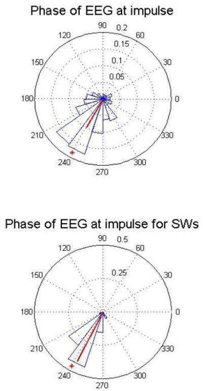
The histogram of the phase when the tone was applied (data from all naps and all the 5 subjects). The red line represents the mean phase vector. Top panel is the statistics for all the tones during N3, bottom panel is the distribution of the phase for events that only include slow waves. The target phase of 240 degrees is indicated by a red asterisk.

The amplitude of the EEG at the acoustic tone when a slow wave was detected as a function of phase is plotted in Fig. 8 (SWS data points for subject 4). The majority (79%) of pulses are in the up-state between 180 and 360 degrees. This is valid for all the pulses even for low amplitudes, when the PLL was not locked. The error becomes small for the higher-amplitude events corresponding to real slow waves.

Fig. 8.

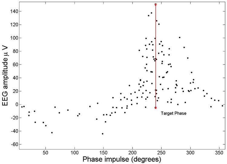
The amplitude of the EEG at the time of the acoustic impulse during SWS for subject 4 is shown as a function of phase. Most of the pulses (79%) where delivered between 180 and 360 degrees that corresponds to the up-state of the slow waves. As the amplitude becomes larger the phase of the impulse comes closer to the target phase of 240 degrees (shown as a red vertical line).

Fig. 9 shows which percentage of pulses are within a radius of 30 degrees from the mean vector in the distribution shown in Fig. 7 top panel as a function of amplitude (all subjects). As we select pulses at higher EEG amplitudes, the percentage increases. For amplitudes above 90 microvolts more than 95% of all the pulses were within 30 degrees from the target phase.

Fig. 9.

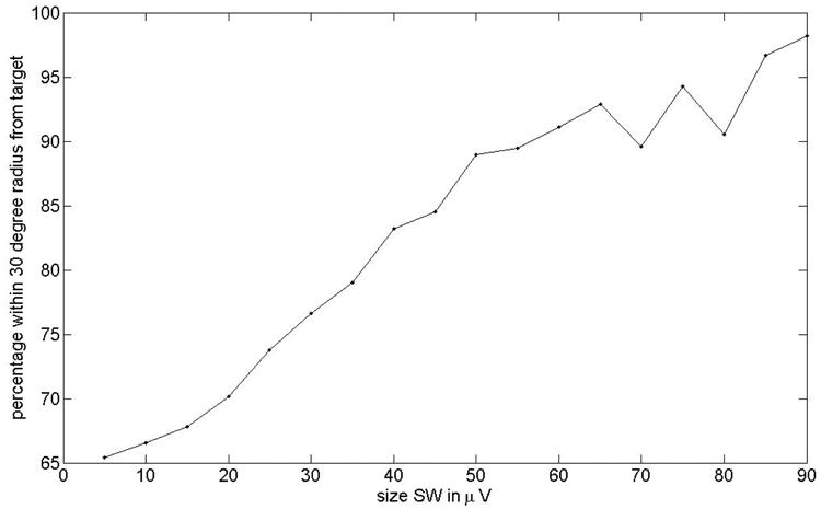
Percentage of that pulses are within a radius of 30 degrees from the mean vector in the distribution shown in Fig. 7 top panel as a function of amplitude (all subjects). For pulses that happened at higher EEG amplitudes the percentage increases. For amplitudes above 90 microvolts more than 95 % of all the pulses are within 30 degrees from the target phase.

The phase and amplitude of the EEG at the time when the acoustic pulses were delivered as measured with the Hilbert transform and the PLL is shown in Fig. 10 (SWS for subject 4). This figure illustrates the relationship between the reference oscillation and the EEG phase. Event time is on the y-axis while the x-axis shows the phases of the acoustic tone in degrees. Most of the pulses, in particular when associated with large slow waves, are in agreement with the phase estimation of the PLL. This outcome could suggest a possible alternative strategy for stimulation that would focus on delivering a stimulus only if a certain amplitude and phase threshold is reached, instead of emphasizing the temporal continuity of the stimulation. As discussed above, we delivered pulses even when the PLL was not locked. Perhaps this strategy may induce slow waves in older adults given they have less SWS; however this may be not appropriate for young subjects. Further experimentation with both approaches is needed to determine which is most efficacious in terms of increasing slow-wave power and coherence for different conditions and subject populations.

Fig. 10.

This diagram shows the relationship between the amplitude of the EEG at the pulse versus the phase of the EEG at the pulse (data from subject 4). The y-axis shows the pulse count (positive values). The pulses have a phase value that is much closer to the estimation of the PLL when the EEG had a large amplitude at the pulse. Most of the pulses are close to the PLL estimated value.

The spectrum of the EEG and the PLL is shown in Fig. 11 (subject 4 data). The PLL has a narrower band than the EEG during in SWS. The two spectra match quite well below 0.8 Hz. The discrepancy is higher for frequencies above 3 Hz.

Fig. 11.

Spectrum of the EEG and the PLL (subject 4 data), showing that the EEG is a narrow-band process during SWS but the PLL is further narrowed around 1 Hz. This graph illustrates that range of sensitivity of the PLL, at frequencies above 3Hz the PLL has much less power than the EEG spectrum so it is not useful to track oscillatory processes above this frequency.

Fig. 12 shows a wavelet scalogram (the output of the wavelet transform where x represents time, y represents scale, and z represents energy) for the PLL superimposed on the EEG slow waves scalogram (only sections of the EEG that contain slow waves were selected as input, data from subject 4 nap) in a 60-s time span. The slow waves were detected using the algorithm described in section 2.4.2. The figure demonstrates how the PLL tends to drift to a frequency of approximately 1.1 Hz between a burst of slow waves, and then follows on short time scales the slow wave oscillations matching the peaks closely. This figure shows in detail that the current realization of the PLL stimulates at a frequency of 1.1 Hz when slow waves are absent and at the particular individual slow wave frequency when a burst of slow wave starts.

Fig. 12.

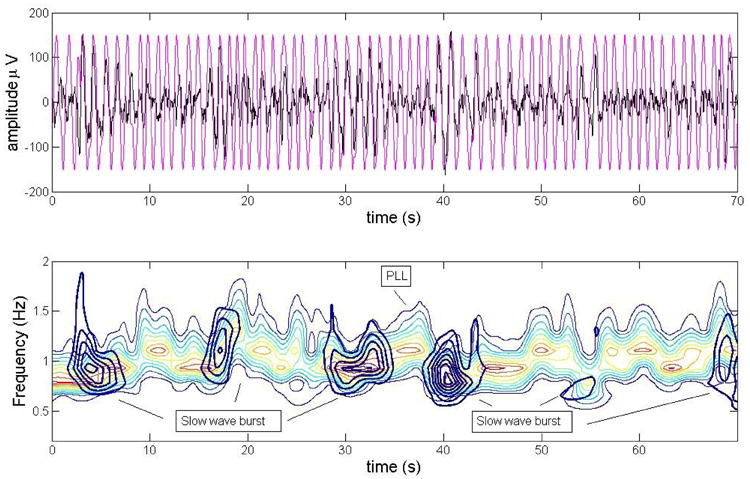
The top panel shows the traces for the PLL (black) and the EEG (pink), the data is from subject 4. The bottom panel is a scalogram (using a Morlet wavelet) contour of the PLL and the single slow waves. The evolution over time of the PLL is illustrated in a color-coded fashion with hot colors indicating high energy values. The monocolor contours represent isolated slow wave bursts, the inner most circles having the highest amplitude values. The figure illustrates how the PLL matches closely the frequency of the slow wave burst in the proper time scales and it can follow the occurrence of slow-wave bursts.

Fig. 13 top panel shows the traces of EEG and the PLL (data from subject 4). The middle panel indicates the correlation between the EEG and the PLL at different frequencies. The correlation is almost 1.0 during slow-wave bursts with a dominant frequency of 0.8 Hz. The bottom panel demonstrates that the phase differences between the two times series is close to zero during bursts of slow-waves (the PLL is locked).

Fig. 13.

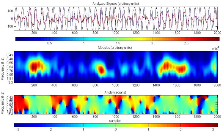
Wavelet coherence of the PLL and the EEG trace. The top panel shows the two traces, EEG (red) and PLL (black), data from subject 4 nap. The middle panel shows the coherence between the two times series. The colors represent wavelet energy with hot colors indicating higher coherence. The bottom panel shows the value of the phase difference in radians. During slow-wave bursts the amplitude coherence reaches values close to 1. The phase is close to zero in the presence of slow-waves bursts, when the PLL is locked. The scale range goes from 1 to 46 or 20 to 0.4 Hz, the center of the graph (where most of the high coherence values are observed) corresponds to 0.8 Hz.

5.4 Comparison of phase targeting with other acoustic stimulation methods

Several algorithms to track and target the phase of the EEG during slow wave sleep have been proposed for online acoustic stimulation [22, 26]. Cox et al. [26] described an algorithm based on Fast Fourier Transform (FFT) calculation, filtering in a given frequency band, measuring of power, Hilbert transform, and fitting to a sine function to create a predictive phase model of the EEG. By inspection of the circular histograms in Cox et al. [26] Fig. 1, it seems that the targeting of the phase is inconsistent from subject to subject, whereas in our case we have similar results for different subjects. The target up-state phase is 90 degrees in Cox et al., while the observed mean vector value for the delivered stimulation is 78.7 ± 65.6 degrees. In comparison, the PLL method gives a mean vector of 243.15 ± 3.06 degrees (with a target phase 240 degrees) in the presence of slow waves.

Ngo et al. [22] proposed a closed loop for stimulation of slow-waves. In this research, a relatively simple but non-adaptive algorithm was used. An average slow-wave duration and amplitude threshold were estimated for each subject, to identify the occurrence of a slow wave. Then, an acoustic pulse of pink noise was used to enhance slow-wave amplitude, as in our approach. Statistical results of the performance of this algorithm in terms of phase tracking and targeting was not given. We have reproduced the algorithm and applied it to the same set of offline data in our experiment to simulate its performance. The results are illustrated in Fig. 14 that compares the performance of our algorithm with the one used by Ngo et al. With a-240 degree target phase, the mean vector of the phase for the Ngo et al. algorithm was 220.73 ± 52.3 degrees (all data for all subjects considered). On the whole, our algorithm is relatively simple to implement (simple algebraic operations), and compared to other options it is more adaptive (can be applied to target many phases and frequencies) and more precise for accurately delivering stimuli phase-locked to the EEG.

Fig. 14.

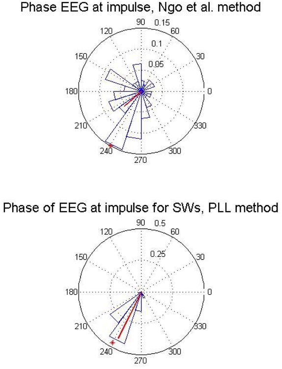
Comparison of the PLL and Ngo et al. algorithms. The top panel shows a circular histogram of the performance of the Ngo et al acoustic closed loop in tracking the phase of the EEG according to a simulated run on the same group of subjects than in our experiment. The bottom panel shows the result in the presence of slow wave for the PLL (real data from all the subjects naps). The target phase is indicated by a red asterisk. The PLL seems is more accurate and precise than the Ngo et al. algorithm.

3.4 Enhancement of slow wave power and synchronization

Our algorithm taps specific resonances in the EEG to allow the brain to drive its own rhythms, corralled within a user-defined bandwidth, in this case the delta power bandwidth. In our nap study, all subjects showed an increase in slow-wave band-limited power (0.5 - 4 Hz) during blocks ON compared to blocks OFF, ranging from 15% to 120%. These stimulated slow waves showed characteristics typical of slow waves normally seen during natural sleep. The topographical distribution of the stimulated slow waves was nearly identical to the distribution of endogenous slow waves of SWS.

These results confirm the viability of using automatically administered acoustic stimulation to enhance slow waves in sleep.

The main goal of this paper is to demonstrate the ability of our algorithm to track the EEG during SWS and determine the phase with a reasonable precision in real time. However, given that one of the main applications of this method will be the enhancement of SWS with useful implications for understanding brain processes and therapeutic applications, we include some preliminary results that demonstrate changes in delta power and synchronization of slow waves. Fig. 15 shows a particularly good response from a young subject during a nap session (subject 4). We calculated the average EEG power from Fpz over 5 seconds, with 50 % overlap and a Hanning window. Power in the delta band increased by more than 100 % in the block ON vs the Block OFF during stimulation (p<0.01) and a non-significant increase in power in the beta band of about 4 % in the beta band.

Fig. 15.

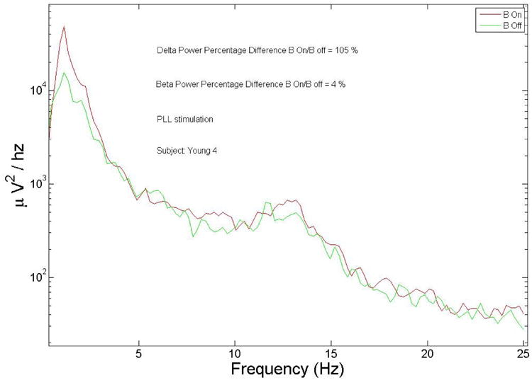
EEG spectrum of a particular responsive young individual (subject 4), a large increase of delta power during the block ON (B On) intervals relative to the block OFF (B Off) intervals during stimulation is clearly visible. The two spectra do not differ significantly in the beta region.

The stimulation protocol also improved synchronization of the slow waves. This increase in synchronization was measured by averaging the EEG event related potentials time-locked to the start of the first tone of each 5-tone block. The results are illustrated in Figure 16 showing the grand average over all 5 subjects. There is a clear increase in average amplitude at each auditory tone even if a decay is observable probably due to a decrease in synchronization for subsequent tones. The difference (using a t-test between each averaged data point) between the two graphs is statistically significant with p<0.01 up to the first 4 auditory pulses.

Fig. 16.

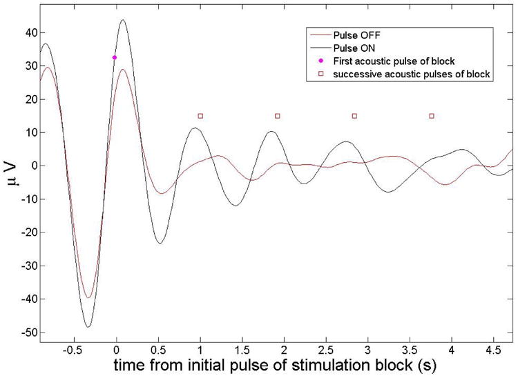
Grand average event related potentials (ERP, grand average over all 5 subjects) for block ON and block OFF intervals (during stimulation), locked to the onset of the first tone of each 5-tone block for Fpz. The ON stimulation case shows more coherence between trials resulting in higher amplitudes at the location of the acoustic pulses. The amplitude of the peaks diminishes for subsequent acoustic pulses (marked with a red square symbol). The subsequent pulses are used here for reference and are separated by the average pulse interval of 1.06 s.

Spectral analysis for all subjects was performed by averaging the power for 4 different conditions using time intervals of 5 seconds during block ON and Block OFF for both the stimulation and the sham condition. Individual spectra were averaged and then smoothed with a 10-point moving average. There was a statistically significant (p<0.05) increase of 15.3 % in power in the delta band between the stimulation and sham conditions. Table 1 shows the statistics for the different EEG bands, and Figure 17 and Figure 18 show the spectrum and zoom in the delta region (average over all the subjects). Given that spectral power during blocks ON and blocks OFF during the sham condition are similar, these two figures include only blocks ON during sham for comparison with blocks ON and blocks OFF during stimulation.

Table 1.

Statistics for EEG band power percentage difference between conditions (averages over all the subjects). The percent change in block ON (stimulation vs sham) was calculated as spectral power of [block ON (stimulation) – block ON (sham)]/[block ON (sham)]. The percent change in block ON vs block OFF during stimulation was calculated as spectral power of [block ON (stimulation) – block OFF (stimulation)]/[block OFF (stimulation)]. Statistical significant results were observed in the delta, theta and fast spindle bands.

EEG band	Percent change in block ON (stimulation vs sham)	Percent change block ON vs block OFF during stimulation Stimulation condition
Delta (0.5-4 hz)	15.3 % p<0.05	52.8 % p<0.01
Theta (4-8 hz)	12.6 % p<0.05	19.3 % p<0.01
Alpha (8-12 hz)	7.4 % p=0.11	7.2 % p=0.08
Fast Spindle (14-16 hz)	19.0 % p<0.05	30.1 % p<0.01
Beta (16-25 hz)	1.55 % p=0.61	1.57 % p=0.59

Fig. 17.

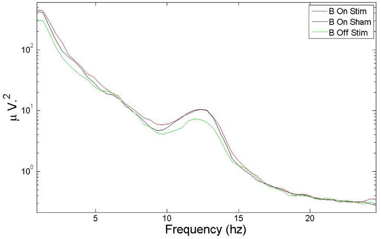
EEG spectrum for 3 different cases blocks ON during stimulation (B On Stim) and sham (B On Sham) and blocks OFF during stimulation (B Off Stim) with all subjects averaged. The main change in power during blocks ON B for the stimulation vs sham conditions was in the delta band.

Fig. 18.

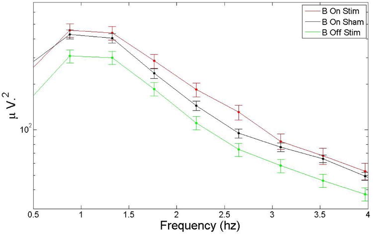
A zoom-in of the EEG spectrum in the delta region. The auditory stimulation produced an increase of 15.3% in delta band. There is a decrease in power during block OFF (B Off) segments, possibly due to a refractory effect.

4 Discussion

The PLL implemented here was effective in tracking slow-waves and determining the correct phase for stimulation. EEG recorded from a frontal electrode during SWS was used as the PLL input, and the phase of the EEG slow-wave oscillations was estimated in real time so that acoustic stimuli could be delivered accurately at a given phase of the EEG.

The phase-locked loops used for most applications operate with small phase errors. These errors are often due either to phase jitter in the input signal or because the loop is made fast enough to follow larger phase excursions with a small lag. The EEG has large phase excursions, but it is not desirable to make the loop response fast because the reference oscillator would then have a broad spectrum of its own which would distort the spectrum of the measured phase. In other words, the PLL in this application should ideally have a slow response, so that the VCO frequency remains steady at the average center frequency of the slow-wave activity.

The choice of VCO gain used here reflects this constraint in our implementation of a PLL. As the same time, as shown in Fig. 12, the PLL can adapt to the presence of sudden bursts of SWA in the characteristic time scale. While the PLL phase estimation is somewhat noisy, it does relatively well, delivering up to 80% of the pulses in this chosen region. When only acoustic pulses that were delivered in the presence of large EEG amplitudes were considered, almost all the pulses happened within a 30-degree radius of the target phase. This suggest that with the addition of a simple amplitude threshold, the PLL can be very accurate in delivering the stimulation at the right phase.

In this way, acoustic pulses can be delivered in a relatively broad range of phases that correspond to different physiological states, particularly the silent down-state or the excitatory up-state of neuronal assembles during SWS. The large range of phase values at which the pulses are delivered versus the mechanically precise rhythm of a perfect sinusoid might be an advantage in stimulating a biological system, given that realistic neural oscillators do not have one precise natural resonant frequency and there would be a range of values for these frequencies.

The ability to reliably enhance SWS is critical to testing relationships between SWS and other physiologic functions. This is particularly important because sleep dysfunction, particularly sleep loss, is endemic in modern society [43], and is common in people with cardio-metabolic disorders such as obesity, hypertension, and diabetes mellitus [5, 44-47]. In particular, SWS has been implicated in regulation of processes such as blood pressure [48], glucose, growth hormone secretion [49], and memory consolidation [50, 51]. Use of methods for selective deprivation of SWS without reduction of total sleep time has provided a deeper understanding of these relationships. For example, selective deprivation of SWS using sounds to cause micro-arousals during SWS has been shown to lead to attenuation of normal dipping of blood pressure during sleep [48] and impaired glucose metabolism [5]. A method such as the PLL will allow us to determine if enhancement of SWS can improve or restore regulation of these functions, particularly if they are already impaired. If this method proves successful, then the acoustic stimulation of SWS could be a novel and non-pharmacologic intervention to treat common diseases with major implications for health.

5 Conclusions

The PLL has been used in many engineering applications, but it has had relatively limited use as a tool for brain stimulation. Here we demonstrated a novel PLL implementation that used online estimation of slow-wave phase to facilitate the regular alternation between the up and down states of cortical activity during SWS. Given the relevance of EEG oscillations for neural function in general, this technique has potential for applications in which enhancement of SWS is desirable, such to improve neurocognitive and cardio-metabolic functions.

Highlights.

• Brain-computer interface to enhance slow wave sleep

• Acoustic stimulation that is effective and non-invasive

• EEG power and synchronization is increased in delta band

• Accurate phase locked algorithm to track phase of EEG during slow wave sleep

• Intervention has potential to enhance benefits of slow wave sleep (memory, metabolism, immune system, cardio-vascular health).

References

- 1.Horne J. Human slow wave sleep: a review and appraisal of recent findings, with implications for sleep functions, and psychiatric illness. Experientia. 1992;48(10):941–54. doi: 10.1007/BF01919141. [DOI] [PubMed] [Google Scholar]
- 2.Diekelmann S, Born J. The memory function of sleep. Nat Rev Neurosci. 2010;11(2):114–26. doi: 10.1038/nrn2762. [DOI] [PubMed] [Google Scholar]
- 3.Mander BA, et al. Prefrontal atrophy, disrupted NREM slow waves and impaired hippocampal-dependent memory in aging. Nat Neurosci. 2013;16(3):357–64. doi: 10.1038/nn.3324. [DOI] [PMC free article] [PubMed] [Google Scholar]
- 4.Westerberg CE, et al. Concurrent impairments in sleep and memory in amnestic mild cognitive impairment. J Int Neuropsychol Soc. 2012;18(3):490–500. doi: 10.1017/S135561771200001X. [DOI] [PMC free article] [PubMed] [Google Scholar]
- 5.Tasali E, et al. Slow-wave sleep and the risk of type 2 diabetes in humans. Proc Natl Acad Sci U S A. 2008;105(3):1044–9. doi: 10.1073/pnas.0706446105. [DOI] [PMC free article] [PubMed] [Google Scholar]
- 6.VanCauter E, Plat L. Physiology of growth hormone secretion during sleep. Journal of Pediatrics. 1996;128(5):S32–S37. doi: 10.1016/s0022-3476(96)70008-2. [DOI] [PubMed] [Google Scholar]
- 7.Xie L, et al. Sleep drives metabolite clearance from the adult brain. Science. 2013;342(6156):373–7. doi: 10.1126/science.1241224. [DOI] [PMC free article] [PubMed] [Google Scholar]
- 8.Gais S, Born J. Declarative memory consolidation: mechanisms acting during human sleep. Learn Mem. 2004;11(6):679–85. doi: 10.1101/lm.80504. [DOI] [PMC free article] [PubMed] [Google Scholar]
- 9.Plihal W, Born J. Effects of early and late nocturnal sleep on declarative and procedural memory. J Cogn Neurosci. 1997;9(4):534–47. doi: 10.1162/jocn.1997.9.4.534. [DOI] [PubMed] [Google Scholar]
- 10.Marshall L, et al. Boosting slow oscillations during sleep potentiates memory. Nature. 2006;444(7119):610–3. doi: 10.1038/nature05278. [DOI] [PubMed] [Google Scholar]
- 11.Marshall L, et al. Transcranial direct current stimulation during sleep improves declarative memory. J Neurosci. 2004;24(44):9985–92. doi: 10.1523/JNEUROSCI.2725-04.2004. [DOI] [PMC free article] [PubMed] [Google Scholar]
- 12.Lang N, et al. How does transcranial DC stimulation of the primary motor cortex alter regional neuronal activity in the human brain? Eur J Neurosci. 2005;22(2):495–504. doi: 10.1111/j.1460-9568.2005.04233.x. [DOI] [PMC free article] [PubMed] [Google Scholar]
- 13.Poreisz C, et al. Safety aspects of transcranial direct current stimulation concerning healthy subjects and patients. Brain Res Bull. 2007;72(4-6):208–14. doi: 10.1016/j.brainresbull.2007.01.004. [DOI] [PubMed] [Google Scholar]
- 14.Amzica F, Steriade M. Cellular substrates and laminar profile of sleep K-complex. Neuroscience. 1998;82(3):671–86. doi: 10.1016/s0306-4522(97)00319-9. [DOI] [PubMed] [Google Scholar]
- 15.Tononi G, et al. Enhancing sleep slow waves with natural stimuli. Medica Mundi. 2010;54(2):73–79. [Google Scholar]
- 16.Ferri R, et al. The slow-wave components of the cyclic alternating pattern (CAP) have a role in sleep-related learning processes. Neuroscience Letters. 2008;432(3):228–231. doi: 10.1016/j.neulet.2007.12.025. [DOI] [PubMed] [Google Scholar]
- 17.Ngo HV, et al. Induction of slow oscillations by rhythmic acoustic stimulation. J Sleep Res. 2013;22(1):22–31. doi: 10.1111/j.1365-2869.2012.01039.x. [DOI] [PubMed] [Google Scholar]
- 18.Dang-Vu TT. Neuronal oscillations in sleep: insights from functional neuroimaging. Neuromolecular Med. 2012;14(3):154–67. doi: 10.1007/s12017-012-8166-1. [DOI] [PubMed] [Google Scholar]
- 19.Ng BS, Logothetis NK, Kayser C. EEG phase patterns reflect the selectivity of neural firing. Cereb Cortex. 2013;23(2):389–98. doi: 10.1093/cercor/bhs031. [DOI] [PubMed] [Google Scholar]
- 20.Schabus M, et al. The Fate of Incoming Stimuli during NREM Sleep is Determined by Spindles and the Phase of the Slow Oscillation. Front Neurol. 2012;3:40. doi: 10.3389/fneur.2012.00040. [DOI] [PMC free article] [PubMed] [Google Scholar]
- 21.Volgushev M, et al. Precise long-range synchronization of activity and silence in neocortical neurons during slow-wave oscillations [corrected] J Neurosci. 2006;26(21):5665–72. doi: 10.1523/JNEUROSCI.0279-06.2006. [DOI] [PMC free article] [PubMed] [Google Scholar]
- 22.Ngo HV, et al. Auditory closed-loop stimulation of the sleep slow oscillation enhances memory. Neuron. 2013;78(3):545–53. doi: 10.1016/j.neuron.2013.03.006. [DOI] [PubMed] [Google Scholar]
- 23.Oudiette D, Santostasi G, Paller KA. Reinforcing rhythms in the sleeping brain with a computerized metronome. Neuron. 2013;78(3):413–5. doi: 10.1016/j.neuron.2013.04.032. [DOI] [PMC free article] [PubMed] [Google Scholar]
- 24.Ong JL, et al. Effecsts of Phase-Locked Acoustic Stimulation During a Nap On EEG Spectra and Declarative Memory Consolidation. doi: 10.1016/j.sleep.2015.10.016. Submitted. [DOI] [PubMed] [Google Scholar]
- 25.Riedner BA, et al. Enhancing slow waves using acoustic stimuli; Society for Neuroscience Meeting poster presentation; 2013. [Google Scholar]
- 26.Cox R, et al. Sound asleep: processing and retention of slow oscillation phase-targeted stimuli. PLoS One. 2014;9(7):e101567. doi: 10.1371/journal.pone.0101567. [DOI] [PMC free article] [PubMed] [Google Scholar]
- 27.Viterbi AJ, Cahn CR. Optimum Coherent Phase + Frequency Demodulation of Class of Modulating Spectra. Ieee Transactions on Space Electronics and Telemetry. 1964;Se10(3):95–&. [Google Scholar]
- 28.Farazian M, Larson LE, Gudem PS. Fast Hopping Frequency Generation in Digital CMOS. New York: Springer-Verlag; 2013. [Google Scholar]
- 29.Talbot DB. A Review of PLL Fundamentals, in Frequency Acquisition Techniques for Phase Locked Loops. John Wiley & Sons, Inc; 2012. pp. 3–15. [Google Scholar]
- 30.Hinze T, et al. Biochemical frequency control by synchronisation of coupled repressilators: an in silico study of modules for circadian clock systems. Comput Intell Neurosci. 2011;2011:262189. doi: 10.1155/2011/262189. [DOI] [PMC free article] [PubMed] [Google Scholar]
- 31.Kimura H, Y N. Circadian rhythm as a phase locked loop. Proc IFAC World Congress. 2005 [Google Scholar]
- 32.Schilling RJ. Control of a Biological Clock with Light. International Journal of Systems Science. 1982;13(5):517–523. [Google Scholar]
- 33.Schilling RJ, Robinson CJ. A Phase-Locked Loop Model of the Response of the Postural Control System to Periodic Platform Motion. Ieee Transactions on Neural Systems and Rehabilitation Engineering. 2010;18(3):274–283. doi: 10.1109/TNSRE.2010.2047593. [DOI] [PMC free article] [PubMed] [Google Scholar]
- 34.Brunner C, et al. Online control of a brain-computer interface using phase synchronization. Ieee Transactions on Biomedical Engineering. 2006;53(12):2501–2506. doi: 10.1109/TBME.2006.881775. [DOI] [PubMed] [Google Scholar]
- 35.Ahissar E, Kleinfeld D. Closed-loop neuronal computations: focus on vibrissa somatosensation in rat. Cereb Cortex. 2003;13(1):53–62. doi: 10.1093/cercor/13.1.53. [DOI] [PubMed] [Google Scholar]
- 36.Hileman RE, Dick DE. Detection of phase characteristics of alpha waves in the electroencephalogram. IEEE Trans Biomed Eng. 1971;18(5):379–82. doi: 10.1109/tbme.1971.4502871. [DOI] [PubMed] [Google Scholar]
- 37.L YY, L PC. Categorization of eeg rhythmic patterns based on pll approach; International Conference on Signal Processing Proceedings; 2000. [Google Scholar]
- 38.Pei-Chen L, Yu-Yun L. Applicability of phase-locked loop to tracking the rhythmic activity in EEG. Circuits, Systems and Signal Processing. 2000;19:171–186. [Google Scholar]
- 39.Broughton R, et al. A phase locked loop device for automatic detection of sleep spindles and stage 2. Electroencephalogr Clin Neurophysiol. 1978;44(5):677–80. doi: 10.1016/0013-4694(78)90134-7. [DOI] [PubMed] [Google Scholar]
- 40.Ferrarelli F, et al. Reduced sleep spindle activity in schizophrenia patients. Am J Psychiatry. 2007;164(3):483–92. doi: 10.1176/ajp.2007.164.3.483. [DOI] [PubMed] [Google Scholar]
- 41.Iber C A.A.o.S.Medicine. The AASM manual for the scoring of sleep and associated events: rules, terminology and technical specifications. Westchester, IL: 2007. [Google Scholar]
- 42.Berens P. CircStat: A MATLAB Toolbox for Circular Statistics. Journal of Statistical Software. 2009;31(10):1–21. [Google Scholar]
- 43.Colten HR, Altevogt BM. Sleep disorders and sleep deprivation: an unmet public health problem. Washington, DC: National Academies Press; 2006. [PubMed] [Google Scholar]
- 44.Leproult R, Van Cauter E. Role of sleep and sleep loss in hormonal release and metabolism. Endocr Dev. 2010;17:11–21. doi: 10.1159/000262524. [DOI] [PMC free article] [PubMed] [Google Scholar]
- 45.Buxton OM, et al. Adverse metabolic consequences in humans of prolonged sleep restriction combined with circadian disruption. Sci Transl Med. 2012;4(129):129ra43. doi: 10.1126/scitranslmed.3003200. [DOI] [PMC free article] [PubMed] [Google Scholar]
- 46.Fung MM, et al. Decreased slow wave sleep increases risk of developing hypertension in elderly men. Hypertension. 2011;58(4):596–603. doi: 10.1161/HYPERTENSIONAHA.111.174409. [DOI] [PMC free article] [PubMed] [Google Scholar]
- 47.Koren D, et al. Sleep architecture and glucose and insulin homeostasis in obese adolescents. Diabetes Care. 2011;34(11):2442–7. doi: 10.2337/dc11-1093. [DOI] [PMC free article] [PubMed] [Google Scholar]
- 48.Sayk F, et al. Effects of selective slow-wave sleep deprivation on nocturnal blood pressure dipping and daytime blood pressure regulation. Am J Physiol Regul Integr Comp Physiol. 2010;298(1):R191–7. doi: 10.1152/ajpregu.00368.2009. [DOI] [PubMed] [Google Scholar]
- 49.Van Cauter E, Leproult R, Plat L. Age-related changes in slow wave sleep and REM sleep and relationship with growth hormone and cortisol levels in healthy men. JAMA. 2000;284(7):861–8. doi: 10.1001/jama.284.7.861. [DOI] [PubMed] [Google Scholar]
- 50.Tononi G, Cirelli C. Sleep and synaptic homeostasis: a hypothesis. Brain Res Bull. 2003;62(2):143–50. doi: 10.1016/j.brainresbull.2003.09.004. [DOI] [PubMed] [Google Scholar]
- 51.Tononi G, Cirelli C. Sleep function and synaptic homeostasis. Sleep Med Rev. 2006;10(1):49–62. doi: 10.1016/j.smrv.2005.05.002. [DOI] [PubMed] [Google Scholar]