Abstract
This paper outlines a comprehensive parametric approach for quantifying mechanical properties of spatially heterogeneous thin biological specimens such as human breast tissue using contact-mode Atomic Force Microscopy. Using inverse finite element (FE) analysis of spherical nanoindentation, the force response from hyperelastic material models is compared with the predicted force response from existing analytical contact models, and a sensitivity study is carried out to assess uniqueness of the inverse FE solution. Furthermore, an automation strategy is proposed to analyze AFM force curves with varying levels of material nonlinearity with minimal user intervention. Implementation of our approach on an elastic map acquired from raster AFM indentation of breast tissue specimens indicates that a judicious combination of analytical and numerical techniques allow more accurate interpretation of AFM indentation data compared to relying on purely analytical contact models, while keeping the computational cost associated an inverse FE solution with reasonable limits. The results reported in this study have several implications in performing unsupervised data analysis on AFM indentation measurements on a wide variety of heterogeneous biomaterials.
Keywords: Atomic force microscopy, Tissue biomechanics, Finite element modeling
INTRODUCTION
Nanoindentation using contact mode Atomic Force Microscopy (AFM) has emerged as a powerful material characterization tool, with applications ranging from elastomeric materials,12 to biological cells18 and tissues.21 In particular, the relevance of quantifying mechanical properties of biomaterials gains prominence in light of the fact that various disease mechanisms might be phenotyped by their biomechanical signatures.26 For instance, human pancreatic cancer epithelial cells,25 and human breast cancerous epithelial cells10 were observed to more deformable compared to their normal counterparts, while similar observations were reproduced at the scale of histological breast tissue.21
The extraction of material properties using AFM is typically accomplished by curve-fitting raw AFM force-indentation data to analytical or numerical models. An ubiquitous contact model is based on Hertzian contact theory,8 wherein force and indentation are related by a power relationship of exponent (1.5 for purely spherical contact). Hertzian theory relies on the assumptions of linear elasticity in the specimen and infinitesimal indentation strains, and analytical corrections have since been proposed to the Hertz contact model wherein these assumptions are relaxed.3,14,24 Numerical techniques involving solution of an inverse finite element (FE) problem has been widely studied in the context of AFM based material characterization.5,9,29
Despite the abundance of analytical and numerical techniques for analyzing AFM force-indentation data proposed in literature, most of these approaches assume that the estimated material properties can be extracted by curve fitting the relevant datasets to a single analytical or numerical model. Relatively less emphasis has been directed towards identifying the underlying material model that characterizes the force-indentation behavior, especially in heterogeneous biomaterials such as tissue specimens. For instance, the human breast tissue specimens studied in this work comprises a highly heterogeneous interwoven framework of functional breast cells surrounded in a collagen-rich stromal tissue environment.21 AFM nanoindentation of such heterogeneous samples result in a diverse set of force-indentation curves, not all of which conform to a given analytical or numerical model.
As such, bulk curve-fitting of AFM force-indentation data to analytical models without accounting for the underlying material heterogeneity is likely to result in inaccurate material characterization. On the other hand, inverse FE solutions, while comparatively attractive due to the availability of a wide range of material libraries in commercial FE packages, can be prohibitively expensive when large datasets need to be analyzed. This is particularly the case when AFM acquired mechanical signatures of cancerous breast tissue specimens are used for histopathological inference purposes. A robust and computationally efficient approach obviating the need for subjective user intervention in specifying the material constitutive model is a critically important component of high-throughput AFM based characterization of biomaterials.
In this context, it is important to note the work of Lin et al.11 in automating AFM data analysis by reducing subjective intervention in (a) identifying the point of contact in AFM force curves and (b) restricting curve fitting to the linear elastic regime (corresponding to the Hertz contact model). However, such methods do not elucidate nonlinear contributions in the AFM measurements, which might reveal potentially interesting mechanical signatures in the tissue response to AFM nanoindentation, thereby providing an additional material characteristic for inference purposes.
In this work, a comprehensive computational strategy utilizing a combination of analytical and numerical techniques is proposed to automate analysis of diverse heterogeneous populations of AFM force-displacement curves. The limits of existing analytical contact models in estimating the elastic modulus from AFM indentation datasets are critically investigated, and nonlinear exponential hyperelastic phenomenological material models are proposed to account for AFM datasets where existing analytical models do not suffice. The proposed approach in this paper is validated on simulated force-indentation datasets, and is subsequently implemented on an elastic map acquired from raster AFM indentation of breast tissue specimens. It should, however, be noted that we have limited the scope of this work to quasistatic indentation loading conditions only.
This paper is organized as follows. In the subsequent Materials and Methods section, the tissue preparation protocol and the AFM experimental setup is described, followed by a critical description of the existing analytical contact models. Then, the finite element model is described, following which, a sensitivity analysis is described to ascertain the uniqueness of the inverse FE solution and an automation strategy for unsupervised data analysis of AFM datasets is proposed. Next, in the Results section, the proposed approach is validated on simulated AFM datasets and then implemented on an elastic map. Finally, we conclude with the discussion of our approach.
MATERIALS AND METHODS
Experimental Setup
AFM Experimental Setup
We used Tissue Microarray (TMA) technology to prepare the samples for AFM indentation. Please refer to21,22 for further details on the tissue preparation protocol.*
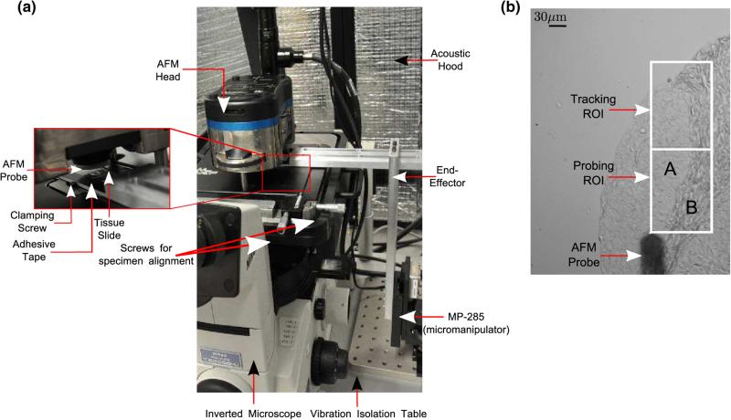
The experimental setup consists of the Atomic Force Microscope (MFP-3D-BIOTM, Asylum Research) and an inverted microscope (Model: TE2000U, Nikon, Inc) with an attached CCD camera (QImaging Inc, Model: Retiga 2000R). The tissue slide is mounted on an end-effector rigidly attached to a 3 DOF motorized micromanipulator (MP- 285, Sutter Instruments, Inc). The AFM, inverted microscope and the micromanipulator are placed on a vibration isolation table to eliminate base vibrations (Fig. 1a). The micromanipulator provides large scan sizes (> 100 μm), beyond the range of commercial AFM scanners.22
FIGURE 1.
(a) and (b) AFM experimental setup with the MP-285 micromanipulator, (c) brightfield image of AFM indentation process. Regions A and B denote epithelial and stromal regions in the “Probing ROI” respectively.
The tissue specimens were aligned with the AFM probe tip using closed loop image-guided positioning prior to AFM indentation. Briefly, a region-of-interest (ROI) was selected by the AFM operator (called the “Probing ROI”), and an adjacent ROI (called the “Tracking ROI”) was used to provide image feedback for tracking purposes (Fig. 1b). A gradient-descent based controller was used to precisely align the the probing location on the tissue specimen and the probe tip within 1 μm. Following accurate positioning, indentations were performed on the “Probing ROI” in a raster fashion. Please refer to22 for further details on the experimental setup.
Contact Model AFM Operation
A schematic of the contact-mode operation of the AFM is shown in Fig. 2a. Briefly, the AFM probe, which consists of a micro-cantilever with an attached particle (often spherical), is lowered towards the specimen using the z-piezoelectric scanner. Based on AFM probe tip and specimen interaction forces, the cantilever deflects, which is then optically sensed. The probe deflection (d) when plotted as a function of the z-position (z) constitutes the (approach) force curve.
FIGURE 2.
(a) Schematic of contact-mode AFM operation, (b) representative AFM force curve and (c) corresponding force-indentation curve.
Given n data points in a force curve, the probe makes contact at (zk, dk) (Fig. 2b). A detailed description of the contact estimation procedure is given in the Appendix. Based on the estimated point of contact, the net indentation in the sample is given by the following equation18:
| (1) |
For low deflection regimes, the cantilever probe is generally approximated as a linear spring of spring constant kc, which is typically calibrated at the start of an AFM experiment. The “thermal method”7 was used for calibrating the probe's spring constant using Asylum Research software (IGOR Pro, Wavemetrics, Inc.). The force, F, then can be related to the deflection by:
| (2) |
The experiments reported in this paper were carried out with an AFM probe of calibrated spring constant 2.23 N/m with a spherical bead of radius R = 2.5 μm (Novascan Technologies, Ames IA).
Contact Models: Finite Indentation and Material Nonlinearity
The classic Hertz contact model relates the contact force, F, with the indentation, Δ, assuming frictionless infinitesimal indentation of an infinitely rigid indenter in a linearly elastic half-space with elastic modulus E and the Poisson ratio v. For a spherical indenter of radius R, the force and indentation are related by8:
| (3) |
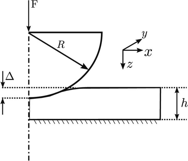
For a specimen of thickness h (Fig. 3), the assumptions of Hertzian contact theory imply the following conditions:
| (4a) |
| (4b) |
| (4c) |
FIGURE 3.
Finite-indentation of a thin specimen by a rigid hemispherical indenter.
The assumptions of infinite specimen thickness (Eq. (4a)) and (Eq. (4b)) pose severe restrictions for analyzing AFM indentation data on thin specimens, such as breast TMAs, which are the subject of this study. Breast TMA specimens are typically sectioned 4 μm - 10 μm (we used 4 μm sections in our experiments) and enforcing Hertzian restrictions necessitate very low indentation ranges close to the noise range of the AFM,13 thereby complicating AFM data analysis.
While it is possible to reduce the bead size R to enforce Hertzian assumptions (Eq. 4c), sharp probe tips with low radius (in the nm-range), can cause permanent damage to the tissue samples.15 Even worse, sharp tips possess the undesirable tendency of including contributions from the substrate,4 leading to inaccurate material characterization. An optimum range of R ~ 5 – 10 μm ensures low stress concentration in the tissue specimens, and also aids on averaging out local tissue heterogeneity.
Due to these practical experimental difficulties, it becomes necessary to account for the inevitable violations in Hertzian assumptions in the contact modeling framework. The most seminal contribution in this field points to the work of Dimitriadis and his co-workers.3 Dimitriadis et al.3 appended correction terms to the Hertz contact model that led to an analytical force-indentation relationship given below:
| (5) |
where E, R, Δ, v have their usual meanings, κ = RΔ/h2 and α0, β0 are constants that depend on the Poisson's ratio v. Note that in the limit κ → 0, Eq. (5) reduces to the classical Hertz contact model. When specimen is bonded to the substrate (for instance, a microscope glass slide), the α0, β0 take the following form3:
| (6a) |
| (6b) |
While Dimitriadis’ model accounts for finite indentation, it retains the Hertzian assumption of linear elasticity in the specimen. Various biomaterials have shown nonlinear hyperelastic indentation response, both at the macroscale16 and microscale.1 To account for material nonlinear effects, Lin et al.13 developed a variety of force-indentation relationships for a variety of hyperelastic material models, however, these do not account for finite indentation effects.
Recently, Long et al.14 extended Dimitriadis approach of appending correction factors to the Hertz contact model by assuming neo-Hookean hyperelastic effects, while finite indentation effects were also included in the modeling framework. Assuming incompressibility in the specimen (v = 0.5), the following force-indentation relationship was obtained:
| (7) |
in the regime Δ/h ≤ min(0.6, R/h) and 0.3 ≤ R/h ≤ 12.7. The constants α1, α2 and γ are depend on h and R. When frictionless contact is assumed, these constants are given by:
| (8a) |
| (8b) |
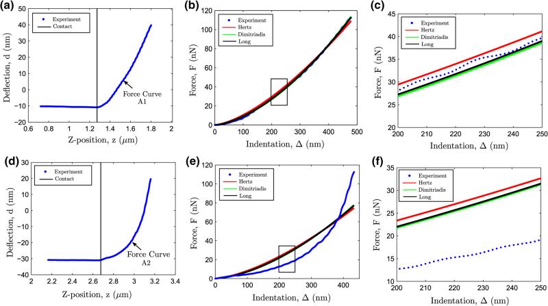
The comparative ability of the Hertz, Dimitriadis and Long contact models in estimating the elastic modulus is demonstrated on two neighborhood sampled points the “Probing ROI” of the breast tissue specimen shown in Fig. 1, leading to force curves termed A1 and A2. Incompressibility conditions (v = 0.5) were assumed in the tissue specimens due to the hydrated nature of the tissue specimens in phosphate buffered saline (PBS) during AFM indentation experiments. The contact point in these forces curves were estimated using a continuity constrained weighted bi-domain polynomial approach (see Appendix).
In force curve A1 (Figs. 4a–c), it is evident that all three contact models fit the deflection data well (R2 ~ 0.999, see Table 1).** However, the Hertz model overestimates the elastic modulus compared to the other two models (see Table 1). This apparent “stiffening effect” from the Hertz model for the case of spherical indentation of thin specimens has been reported elsewhere19 and it has been attributed to the effect of the rigid substrate underneath the thin specimen. It can also be observed that the estimated elastic modulus using both Dimitriadis and Long's model are close to each other. This is explained by observing that the Long's model reproduces the result from Dimitriadis model for indentation regimes D/h close to 0.114 (neo-Hookean hyperelasticity is nearly “Hookean”, i.e., linearly elastic, for low deformation).
FIGURE 4.
Comparative performance of the Hertz, Dimitriadis and Long's contact models on two AFM force curves A1 (a–c) and A2 (d–f).
TABLE 1.
Extracted elastic modulus from force curves A1 and A2 using Hertz, Dimitriadis and Long contact models.
| Elastic modulus (kPa) | Indentation (nm) | R 2 | ||
|---|---|---|---|---|
| Force | Hertz | 117.6 | 461.8 | 0.999 |
| Curve | Dimitriadis | 86.0 | 461.8 | 0.999 |
| A1 | Long | 89.1 | 461.8 | 0.999 |
| Force | Hertz | 93.0 | 433.1 | 0.845 |
| Curve | Dimitriadis | 70.1 | 433.1 | 0.874 |
| A2 | Long | 72.3 | 433.1 | 0.869 |
For force curve A2 (Figs. 4d–f), none of the aforementioned contact models produce a good fit (R2 varies from 0.845 to 0.874), despite the indentation range being nearly equal to that for force curve A1. Such heterogeneous indentation response is typical of heterogeneous biological samples such as human breast tissue, where analytical contact models do not describe all force curves acquired on a tissue region-of-interest. Force curves such as A2 indicate significant material nonlinearity beyond neo-Hookean hyperelasticity, and numerical techniques with higher order hyperelastic material formulations are necessary, as discussed in the subsequent section.
Finite Element Modeling
Meshing and Boundary Conditions
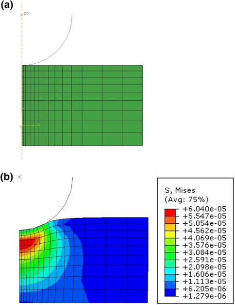
The FE analysis of spherical nanoindentation was carried out in ABAQUS v6.8 (Dassault Systemes, RI, USA). Taking advantage of the symmetry of the indentation process, a 2D axisymmetric model of the indenter and the tissue specimen was used. The quarter of the spherical indenter in contact with the specimen was modeled as an analytical rigid element. The contact force from the simulations was obtained at a reference node attached to the spherical indenter.
The tissue specimen consists of 135 axisymmetric, quadrilateral hybrid elements (CAX4H) (15 radially, 9 axially). The length of the tissue model was 6 μm. A fine mesh was used near the indentation region, with a coarser mesh away from it (see Fig. 5). No friction was assumed between the indenter and the tissue specimen model. The nodes at the interface of the specimen and the indenter were considered traction free, while the nodal displacements in the radial and axial directions were constrained. Nodes on the axis were constrained to move only along the direction of indentation. Quasistatic equilibrium solutions were acquired for incremental axial displacements of the indenter. In a mesh convergence study, we verified that mesh size or the length of the tissue model did not have significant impact on the analysis results.
FIGURE 5.
Finite element models: (a) undeformed mesh, (b) deformed mesh.
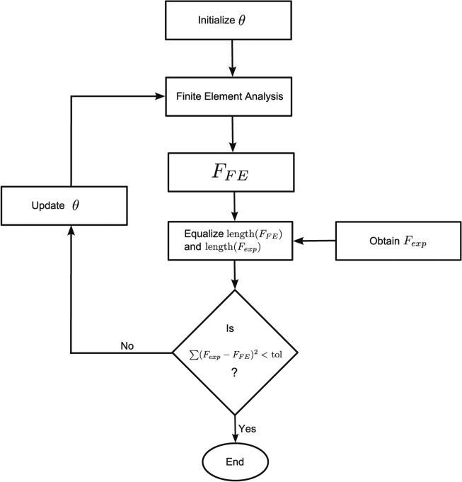
With any single or multi-parameter constitutive model whose explicit force-indentation relationship is unknown, estimating the material properties typically involves solution of an inverse-FE problem where the simulated response is curve-fitted to experimental data. This is obtained by minimizing the squared norm of the residuals and is given by the following expression:
| (9) |
where Fexp and FFE represent the experimental and simulated force response respectively, and θ represents a vector of material parameters defined in the constitutive material model. The minimization problem was implemented in MATLAB (Mathworks, Inc) using the fminsearch routine which is a heuristic optimizer using the Nelder-Mead simplex algorithm.17 The optimizer iterates from an arbitrary initial point towards the optimum solution until the incremental reduction in the objective function is lesser than a predefined tolerance. A flowchart indicating the steps of the inverse FE approach is shown in Fig. 6.
FIGURE 6.
Flowchart of the algorithm used to obtain optimized material properties using the inverse FE approach.
Constitutive Material Models
In order to model force curves like force curve A2 shown in Figs. 4d–f, significant material nonlinearity needs to be considered in the constitutive material model. We examine the force response for the following two incompressible hyperelastic materials characterized by the following strain energy functions.
| (10a) |
| (10b) |
where (C1, C2, C3) and (C, b) are hyperelastic material parameters of the Yeoh and Fung hyperelastic models respectively and I1 is the first invariant of the Cauchy-Green deformation tensor, expressed in terms of the principal stretch ratio λ1, λ2, λ3 as:
| (11) |
where λ1λ2λ3 = 1 for incompressible conditions to hold. Eq. (10a) represents the Yeoh hyperelastic material28 which can be viewed as a polynomial extension of the neo-Hookean model (with C2, C3 = 0), and is commonly used to model rubber elasticity. Eq. (10b) represents an exponential form proposed by Fung,6 which has been previously used to model biomaterials. The presence of higher orders coefficients such as (C2, C3) and b is the Yeoh and Fung models respectively makes these two models particularly attractive in describing highly nonlinear force curves such as A2 (Figs. 4d–f). While the Yeoh material model was pre-defined in the ABAQUS material library, Fung's model was not. Consequently, the user subroutine UHYPER was employed to specify the strain energy function denoted by Eq. (10b) for the FE analysis.
The hyperelastic coefficients can be related to the specimen's materials properties using the relation:
| (12a) |
| (12b) |
where μ0 is the initial shear modulus, which is related to the initial elastic modulus E0 by:
| (13) |
When incompressibility conditions (v = 0.499) apply, E0 = 6C1 and E0 = 6C for Yeoh and Fung material models respectively.
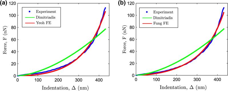
Figure 7 shows the force curve A2 from Figs. 4d–f overlaid with FE simulation results of indentation on a Yeoh (Fig. 7a) and Fung hyperelastic material (Fig. 7b). The results demonstrate the applicability of higher order hyperelastic material models to reproduce force curves with pronounced nonlinearity (R2 > 0.99). The estimated hyperelastic parameters using an inverse FE analysis were (C1, C2, C3) = (1.81, 112.3, 4049.8) kPa and (C, b) = (4.18 kPa, 46.94) for the Yeoh and Fung hyperelastic models respectively. Using Eq. (13), the initial elastic modulus was compute to be E0 = 10.80 for Yeoh's model and E0 = 25.08 kPa for Fung's model.
FIGURE 7.
Performance of the (a) Yeoh and (b) Fung hyperelastic models in describing the force response for force curve shown A2 in Figs. 4d–f.
The quality of fit being similar for both the Yeoh and Fung hyperelastic models, a pertinent question comes up: which hyperelastic model should be selected for modeling force curves shown in Fig. 7.
In this context, the Fung model is appears particularly attractive because of one less hyperelastic parameter compared to the Yeoh model. From the perspective of solving an inverse-FE problem, it is also likely that the Fung model would pose less existence and uniqueness problems compared to the Yeoh model, where material nonlinearity is coupled in between C2 and C3. In contrast, Fung's model is fairly decoupled: C quantifies the initial elastic modulus, while b describes the degree of material nonlinearity. For these reasons, the Fung hyperelastic model is used to describe the observed nonlinear hyperelasticity in the AFM force curves such as force curve A2.
Sensitivity Analysis
The estimated value of b (= 46.94) in Fig. 7 raises another interesting question: is there an existence of a lower bound of b which corresponds to a linear elastic response (the analytical analogue of which is Dimitriadis model) ? If this is the case, then the parameter b could be used to potentially differentiate between linear and nonlinear elastic responses in the tissue specimen, which could serve as an additional mechanical signature for tissue health.
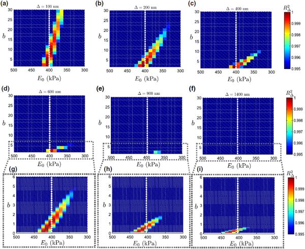
A sensitivity analysis is performed to examine values of E0(= 6C) and b that resulted in a good fit with a F – Δ curve obtained from a linearly elastic material, and the results are shown in Fig. 8. The target F – Δ curve was obtained by varying the indentation from Δ = 100 nm to D = 1400 nm on a linearly elastic specimen of elastic modulus 400 kPa and 4 μm thickness.
FIGURE 8.
Sensitivity of the Fung model parameters at varying indentations. (a) Δ = 100 nm, (b) Δ = 200 nm, (c) Δ = 400 nm, (d) Δ = 600 nm, (e) Δ = 900 nm and (f) Δ = 1400 nm. Also shown in the third row (g–i) are enlarged figures of (d–f) where the range of b is reduced to 1 – 6. The white dotted line at 400 kPa indicates the elastic modulus of the linearly elastic material.
The ranges of E0 and b that fit well with the linearly elastic force response can be compactly expressed by the region where , where indicates a pre-specified threshold R-square value. The term has implications for an inverse FE analysis during parameter estimation - it determines the termination criteria for an inverse FE solution. In Fig. 8, was chosen to be 0.995 (see colorbar in Fig. 8).†
For low indentation regimes such as Δ = 100 nm, (Fig. 8a), moderately hyperelastic specimens (b ~ 25 – 30)‡ produce a linearly elastic resposne. With increasing Δ, the domain of progressively shrinks. The immediate implication of this observation in that parameter estimation using an inverse FE approach is likely to yield inaccurate estimates of b for shallow indentation regimes due to the relatively large domain of leading to solution multiplicity and it is unlikely that it would be possible to differentiate between linear and hyperelastic tissue response for these regimes.
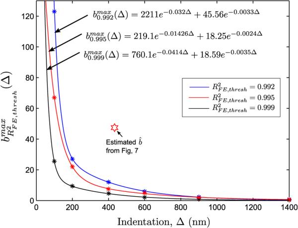
However, for larger indentations, the estimated values of b can be used for differentiating between linear and hyperelastic tissue response. This is evident by observing that for an indentation of Δ = 433.1 nm in force curve A2 of Fig. 7, the estimated b was 46.94, whereas the b is upper-bounded in S(400,0.995) by a value of 10-10.5 (see Fig. 8c).
It now becomes possible to construct a classification curve (see Fig. 9), where the linearly elastic tissue response is bounded by (Δ), which is defined as:
| (14) |
FIGURE 9.
Classification curve, showing the variation of (Δ) with Δ for different values of . Also shown are the curve fits for (Δ).
Automation Strategy
The sensitivity analysis discussed in the previous section indicates that the inverse FE solution successfully estimates the elastic modulus from an AFM force curve with linear elasticity through the parameter E0. However, implementing an inverse FE analysis on such force curves is clearly unnecessary, since the Dimitriadis solution suffices. For analyzing force curves with varying degrees on nonlinearity on heterogeneous AFM datasets, the following strategy is proposed (see Algorithm 1).
Algorithm 1.
| input : AFM force curve, , . |
| output: Material parameters |
| Multiply deflection with probe spring constant to obtain force; |
| Contact Estimation: Estimate contact point using weighted constrained BDP; |
| Dimitriadis Curve fitting: Fit F – Δ to Dimitriadis contact model to obtain EDim, ; |
| if then |
| Linear Elasticity: Estimated material parameter: Ê ← EDim; |
| else |
| Hyperelasticity: initialize C0 ← EDim/6, b ← 30; |
| Invoke Inverse FE routine with ; |
| Estimated material parameters: Ê0 ← 6Ĉ0, b̂; |
| end |
The criteria for invocation of an inverse FE correction can be expressed through a threshold R2 parameter: . If a Dimitriadis curve fit for a given AFM force curve is lower than the threshold , an inverse FE correction is invoked, which is terminated when the reaches the threshold .
RESULTS
In this section, the automation strategy proposed in the Materials and Methods section is implemented on AFM force curves of varying degrees of elasticity. Our approach is first validated on simulated force curves to determine its accuracy in estimating the predefined material parameters from heterogeneous force curves. Then, the performance of the proposed approach is then demonstrated on a tissue elastic map.
Parameter Re-identification on Simulated Data
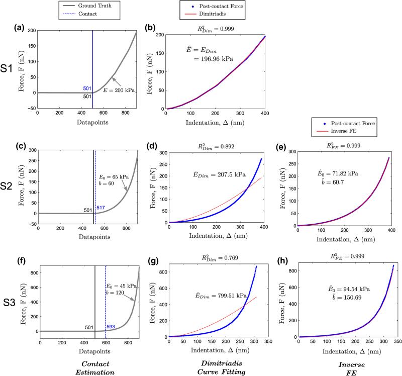
Three AFM force curves are simulated with varying degrees of hyperelasticity. The parameters used to construct force curves are given in Table 2. Additionally, the force values were perturbed by Gaussian noise [~ N(0, 0.05)]. The simulated force curve parameters were re-identified by implementing the proposed automation strategy. The weighting parameters used in the continuity constrained weighted BDP contact estimation technique were w0 = 30, σi = 3. The threshold parameters were set to and respectively.
TABLE 2.
Parameters used to construct the simulated force curves.
| (Contact k, datapoints n) | Indentation (nm) | Linear elastic modulus | Hyperelastic parameters (E0, b) | |
|---|---|---|---|---|
| Force curve S1 | (501,900) | 400 | 200 kPa | × |
| Force curve S2 | (501,900) | 400 | × | (65 kPa,60) |
| Force curve S2 | (501,900) | 400 | × | (45 kPa,120) |
When the material is linearly elastic (force curve S1), the contact point is accurately estimated (see (Fig. 10a), also Table 3), and the Dimitriadis solution (Fig. 10b) is very close to the ground truth (~ 1.5% error, potentially arising from discretization errors).
FIGURE 10.
Implementation of the proposed algorithm for automated characterization for simulated force curves S1 - S3 (shown row-wise). Note that the inverse FE step was not required for curve S1.
TABLE 3.
Summary of algorithm performance on force curves S1-S3. Units of E and E0 are in kPa. G.T. indicates ground truth.
| Force Curve | Contact point
k |
Material parameters |
||||||
|---|---|---|---|---|---|---|---|---|
| G.T. (k) | G.T. (E) | (EDim) | G.T. (E0) | (Ê0) | G.T. (b) | |||
| S1 | 501 | 501 | 200 | 196.97 | × | × | × | × |
| S2 | 501 | 517 | × | × | 65 | 74.87 | 60 | 61.43 |
| S3 | 501 | 593 | × | × | 45 | 94.54 | 120 | 150.69 |
The inverse FE correction step was necessary for force curves S2 and S3. For force curve S2 with moderate hyperelasticity, the estimation errors in E0 and b were 15.13% and 2.33% respectively. For force curve S3 displaying very sharp nonlinearity, the estimation errors in E0 and b are approximately 110.01% and 25.58% respectively. The errors in these two force curves were a direct consequence of the contact estimation error due to the extremely smooth nature of the transition between the non-contact and the contact regime (Figs. 10c, f). This is also evident by noting that the estimation errors were greater in E0 compared to b. Nevertheless, the inverse FE prediction is a marked improvement over the Dimitriadis solution, which overestimates the elastic modulus by approximately 219.23% and 1676.68% for force curves S2 and S3 respectively, thus demonstrating the need to incorporate inverse FE corrections in AFM force curve analysis.
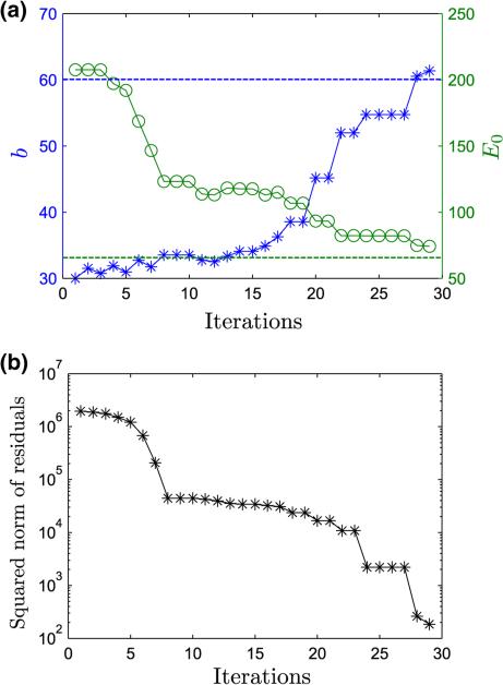
The convergence history of the inverse FE solution is shown in Fig. 11.
FIGURE 11.
(a) Convergence history of the inverse FE solution on force curve S2. Also shown in dotted blue and green are the ground truths for b(= 60) and E0(= 65) kPa respectively. (b) Minimization of the squared norm of residuals.
Implementation on Elastic Map
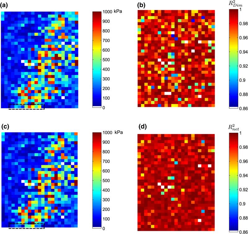
Next, the proposed strategy for automated AFM data analysis is implemented on 729§ force curves acquired at 5μm intervals in the “Probing ROI” 115μm × 160μm in size (see Fig. 1b). This tissue ROI displays a heterogeneous composition of epithelial tissue in the upper left and lower right of the ROI, with the rest of the region corresponding to fibrous stroma. The force curves were acquired at a constant loading force of 120 nN, leading to approximately 85 - 900 nm tissue indentation, depending on its relative stiffness. Due to the computational cost involved in an inverse-FE routine, a modest termination criteria for the inverse-FE procedure was set , while was used for detecting linear elasticity in the force curve.
Figure 12a shows the elastic map of the probing ROI when no inverse FE corrections are implemented, i.e. the Dimitriadis model is used to fit all the force curves after contact estimation. There is fairly good delineation in the computed elastic map, with the epithelial regions displaying lesser stiffness compared to the stroma, a finding observed previously.21 Figure 12c shows the elastic map constructed after the inverse FE routine is implemented. Note the difference in the individual pixel intensities in the first row of the elastic maps in Fig. 12a and c. It can be observed, however, that the overall spatial delineation in the elastic maps do not vary much between Figs. 12a and c. This is primarily due to the fact that the difference in elastic modulus between epithelial and stromal regions is appreciable21 and the colorscale in these figures have been shown from 0 to 1000 kPa to highlight this delineation.
FIGURE 12.
Implementation of the proposed algorithm for automated characterization on a tissue ROI shown previously in Fig. 1b. (a) Elastic map using the Dimitriadis model only without any Inverse FE corrections, (b) Corresponding fit, (c) Elastic map (Ê) with inverse-FE correction, (d) Corresponding fit, where . White spaces indicate uninterpretable force curves that were not analyzed.
However, the efficacy of the inverse FE based approach becomes evident by noting comparing spatial distribution of the corresponding R-square in both cases. in Fig. 12b shows that the fit quality is moderately non-uniform due to the inapplicability of Dimitriadis contact model in describing all the force curves. When the inverse FE routine is invoked (Figs. 12c, d), the R-square distribution improves significantly, because force curves with material nonlinearity are now accounted for using Fung's hyperelastic parameters.
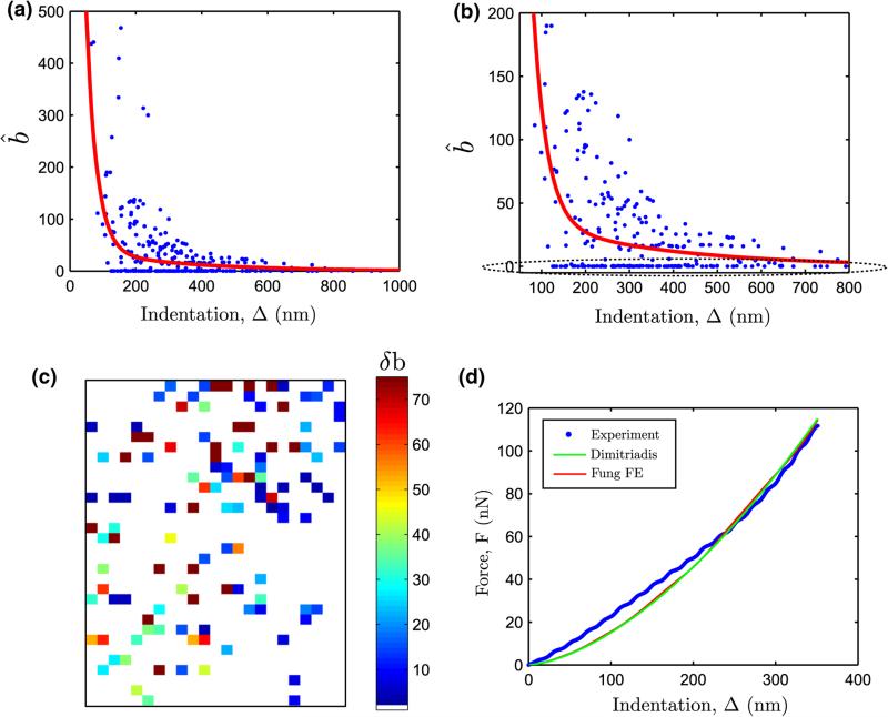
Figure 13 shows the estimated Fung parameter b as a function of indentation for 268 force curves out of a total of 729 force curves analyzed using the inverse-FE routine. Also shown in bold red is the classification curve for a linearly elastic response obtained from the sensitivity study. It can be seen from Figs. 13a, b that the nonlinear hyperelastic force curves can be clearly differentiated from the predicted linear elastic response by classification curve. The degree of nonlienar hyperelasticity can be observed by noting the deviation of b̂ from the predicted linear response, i.e. , δb > 0, at a given indentation depth. The spatial distribution of δb is shown in Fig. 13c. A total of 117 force curves (about 15% of all force curves) registered nonlinear hyperelastic behavior (δb > 0).
FIGURE 13.
(a) Variation of estimated Fung parameter b̂ from the Inverse FE analysis as a function of the estimated indentation (using the contact estimate), (b) zoomed image. Also overlaid in red is , (c) deviation δb in the elastic map and (d) representative force-indentation plot with low estimated b value (Ê0, b̂) = (153.21 kPa, 0.005). Dimitriadis fit quality , Inverse FE fit quality .
On closer examination of Fig. 13b, it becomes apparent that there was a significant population of force curves that showed very low estimates (~ 0.001 – 0.1) in parameter b. Furthermore, such force curves were acquired at all indentation ranges, thus indicating that these force curves were not correlated with a particular tissue stiffness. One such representative force curve is shown in Fig. 13d. These force curves show surprisingly linear force-indentation curves, which can most likely be attributed to material softenting during AFM loading. These force curves did not fit well even after invocation of the inverse-FE routine.
DISCUSSION
While significant research in the past has been directed towards quantifying mechanical properties from AFM force-indentation datasets using analytical or computational means, relatively fewer literature focus on developing accurate modeling techniques that account for heterogeneity in the indentation response of specimens, such as human breast tissue. This has applications mechanical characterization for biological inference studies, where traditional analytical contact models do not account for all force curves in a raster indentation dataset. This paper presents a comprehensive framework of estimating the material properties reliably from diverse populations of AFM force curves. A two-parameter exponential hyperelastic material model is used to account for force curves where analytical contact models fail. An automation approach is suggested, which considerably reduces subjective human intervention in analyzing large AFM datasets, wherein only two R-square threshold parameters (, ) need to be user-specified. The proposed approach is first validated on simulated AFM datasets, and subsequently implemented on an elastic map.
At this point, a few comments are pertinent. In this work, a constant value of the indenter radius (R = 2.5μm) and the specimen thickness (h = 4μm) was used for the experiments and simulations. Varying the indenter size and the specimen thickness is likely to impact the results of the sensitivity studies in the Materials and Methods section. However, the variations in R and h would at most lead to a vertical displacement of the classification curve - the asymptotic nature of the classification curve in Fig. 9 is likely to remain unaltered. It would still be possible to differentiate between a linearly elastic (Dimitriadis) and an hyperelastic tissue response based on the modified Fung parameter, b̂ from the inverse FE analysis, and therefore the major conclusions of this study are independent of the indenter size and the tissue thickness.
It is to be noted here that the aim of this work was to develop a generalized computational approach for mechanical characterization of heterogeneous specimens, not as much to investigate elasticity variations in a specific biological material. As discussed previously in the Results section, the elastic maps in Figs. 12a, c show similar delineation between the epithelial and stromal tissue subtypes even after inverse FE corrections, due to the relatively large elasticity difference epithelial and stromal tissue subtypes, possibly significant enough to be analyzed purely using Dimitriadis contact models and still result in reasonably accurate characterization performance. However, in cases where the elasticity measures between two biospecimens do not differ much, such as, in benign and cancerous epithelial tissue,21 there is a large possibility of erroneous inferences if the absolute elastic modulus is not captured using the proposed (or similar) approaches outlined in this paper. As discussed previously, the Dimitriadis contact model overestimates the elastic modulus by 219.23% and 1678.78% for force curves with moderate (b = 40) to high (b = 120) degrees of nonlinear elasticity. Noting that the mechanical signatures are typically used in a statistical hypothesis test such as the Students t-test, it is quite reasonable to expect incorrect inference when the computed p-values are close to the level of significance, α, if there are significant populations of nonlinearly elastic force curves. This motivates our study to quantify the absolute elastic modulus in spatially heterogeneous biological specimens such as breast tissue using a dedicated Fung hyperelastic constitutive model.
While an inverse FE analysis with Fung hyperelasticity successfully accounted for sharply nonlinear force-curves in the elastic map shown in Fig. 12, there were large populations of force curves (very low estimates (~ 0.001 – 0.1 in parameter b) that could still not be accounted for. These suggest that an alternative material modeling formulations need to be incorporated in the automation strategy proposed in this paper. This remains a subject of future work.
Finally, it should be mentioned here that despite the advantages that a inverse FE approach provide, it is nevertheless computationally expensive with several numerical issues. Such methods have inherent existence and uniqueness problems, especially when the initial conditions for the numerical optimization are improperly set. Approximate analytical contact models that account for Fung hyperelasticity and finite indentation effects on the lines of Dimitriadis3 and Long14 would be particularly attractive in reducing the computational burden of analysing heterogeneous large AFM datasets as shown in Fig. 12. One of the additional advantages of using a purely analytical approach is that it would become possible to integrate uncertainty quantification techniques in AFM data analysis that accounts of inherent variabilities in AFM experimental parameters, such as the AFM spring constant,20,27 and the AFM photodiode sensitivity,27 which assume that an analytical contact model is known. Such methods would further extend the viability and impact of the approach discussed in this paper.
ACKNOWLEDGMENTS
Research reported in this publication was supported by the National Cancer Institute of the National Institutes of Health under Award Number R01CA161375. The content is solely the responsibility of the authors and does not necessarily represent the official views of the National Institutes of Health. The authors would like to thank Dr. Wenjin Chen and Lei Cong from Rutgers Robert Wood Johnson Medical School, New Brunswick, NJ for providing the breast TMA specimens.
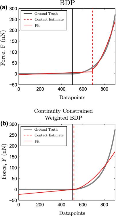
APPENDIX: CONTACT ESTIMATION USING CONTINUITY CONSTRAINED WEIGHTED BDP
The contact estimation procedure used in this work is a modification of the bi-domain polynomial (BDP) approach proposed by Costa et al.,2 a probabilistic extension of which has been recently explored by Rudoy et al.23 This approach relies on the assumption that the AFM force curve can be successfully segmented into a non-contact and contact region, governed by a two-regime regression model, as stated below:
| (A1) |
where Fi is the observed force obtained by multiplying the deflection di by the probe spring constant kc, δi is the probe deflection d subtracted from z-position z, i.e. δi = zi – di. β1 = [β11 β12]T and β2 = [β21 β22]T are the pre-contact and post-contact regression coefficients respectively, k ∈ (1, n) is the unknown contact index for n datapoints, , are the error terms in the pre-contact and post-contact regimes respectively, and fi is the contact model.
The bidomain polynomial (BDP) approach seeks to obtain optimal estimates (k̂, , ) that minimizes the error between the observed force readings Fi and the fitted force estimates from the regression model of Eq. (A1).
In the traditional BDP approach proposed by Costa et al.,2 no continuity was considered at the change-point, i.e. β21 is not necessarily equal to β11 + δkβ12. Observed AFM force curves typically display a smooth transition at the contact point, consequently, a modification to the traditional BDP approach2 is proposed with continuity enforced at the contact point. This leads to the following constraint:
| (A2) |
Due to the constraint in Eq. (A2), the regression parameter space reduces to three unknowns: . The modified regression model from Eq. (A1) are given by the following equations:
| (A3) |
In vector form, these equations are given as:
Furthermore, since existing contact models, fi, are unlikely to fit the entire post-contact force data for highly nonlinear force curves, weights are added to the residuals of the regression model to restrict the fitting range near the contact transition. This is accomplished by defining a diagonal weight matrix where .
The weights, assumed Gaussian, are given as follows:
| (A4) |
Due to the concentration of weights around the candidate contact point k in Eq. (A4), fitting the two-regime model to AFM force curves is restricted to the vicinity of the true contact transition. We used values of w0 = 30 and σw = 3 for contact estimation in this work.
The optimal regression coefficient estimate for a given contact point k is given by:
| (A5) |
The weighted least squares solution is given by:
| (A6) |
The contact point obtained by performing a line search on the sum of squared residuals (SSR) and is given by:
| (A7) |
where
| (A8) |
The efficacy of the traditional BDP and the modified continuity-constrained weighted BDP is shown in Fig. A1, wherein both approaches are implemented on simulated force curve S2 with E0 = 65 kPa, b = 60 (see Table 2). The Dimitriadis contact model was used to specify fi. It is clear that for nonlinear hyperelastic force curves, the continuity-constrained weighted BDP outperforms the traditional BDP in estimating the true contact point.
FIGURE A1.
Performance of the traditional BDP (a) and the continuity-constrained weighted BDP approach in estimating the contact point in simulated force curve S2 with known ground truth. Also shown in solid red are the pre-contact and contact regime fits from the regression model of Eq. (A1).
Footnotes
Note: IRB has determined that the work done on this project does not meet the definition of human subject research.
R-square was computed as R2 = 1 – ∥Fexp – Ffit∥2/∥Fexp – mean(Fexp)∥2.
Minimizing the squared norm of the residuals is equivalent to maximizing the R2.
The peak b at Δ = 100nm was 67.0 for (not shown).
Out of a total of 736 force curves, 7 were uninterpretatble due to improper contact between the probe and the tisse specimen.
The authors report no conflict of interest.
REFERENCES
- 1.Bernick KP, Prevost TP, Suresh S, Socrate S. Biomechanics of single cortical neurons. Acta Biomater. 2011;7(3):1210–1219. doi: 10.1016/j.actbio.2010.10.018. [DOI] [PMC free article] [PubMed] [Google Scholar]
- 2.Costa KD, Smith AJ, Yin FCP. Non-Hertzian approach to analyzing mechanical properties of endothelial cells probed by atomic force microscopy. J. Biomech. Eng. 2006;128(2):176–184. doi: 10.1115/1.2165690. [DOI] [PubMed] [Google Scholar]
- 3.Dimitriadis EK, Horkay F, Maresca J, Kachar B, Chadwick RS. Determination of elastic moduli of thin layers of soft material using the atomic force microscope. Biophys. J. 2002;82(5):2798–2810. doi: 10.1016/S0006-3495(02)75620-8. [DOI] [PMC free article] [PubMed] [Google Scholar]
- 4.Domke J, Radmacher M. Measuring the elastic properties of thin polymer films with the atomic force microscope. Langmuir. 1998;14:3320–3325. [Google Scholar]
- 5.Frassanito MC, Lamberti L, Boccaccio A, Pappalettere C. Discussion on hybrid approach to determination of cell elastic properties. Optical Measurements, Modeling, and Metrology, Volume 5, Conference Proceedings of the Society for Experimental Mechanics Series. 2011:119–124. [Google Scholar]
- 6.Fung YC. Biomechanics: Mechanical Properties of Living Tissues. 2nd edn. Springer; Berlin: 1993. [Google Scholar]
- 7.Hutter JL, Bechhoeffer J. Calibration of atomic-force microscope tips. Rev.Sci. Instrum. 1993;64(7):1868–1873. [Google Scholar]
- 8.Johnson KL. One hundred years of hertz contact. Proc. Inst. Mech. Eng. 1982;196(1):363–378. [Google Scholar]
- 9.Ladjal H, Hanus J-L, Pillarisetti A, Keefer C, Ferreira A, Desai JP. Atomic force microscopy-based single-cell indentation: experimentation and finite element simulation. IEEE/RSJ International Conference on Intelligent Robots and Systems. 2009:1326–1332. [Google Scholar]
- 10.Li QS, Lee GYH, Ong CN, Lim CT. AFM indentation study of breast cancer cells. Biochem. Biophys. Res. Commun. 2008;374(4):609–613. doi: 10.1016/j.bbrc.2008.07.078. [DOI] [PubMed] [Google Scholar]
- 11.Lin DC, Dimitriadis EK, Horkay F. Robust strategies for automated AFM force curve analysis-I. Non-adhesive Indentation of soft, Inhomogeneous materials. Trans. ASME. 2007;129(3):430–440. doi: 10.1115/1.2720924. [DOI] [PubMed] [Google Scholar]
- 12.Lin DC, Shreiber DI, Dimitriadis EK, Horkay F. Elasticity of rubber-like materials measured by AFM nanoindentation. eXPRESS Polym. Lett. 2007;1(9):576–584. [Google Scholar]
- 13.Lin DC, Shreiber DI, Dimitriadis EK, Horkay F. Spherical indentation of soft matter beyond the Hertzian regime: numerical and experimental validation of hyperelastic models. Biomech. Model Mechanobiol. 2009;8(5):345–358. doi: 10.1007/s10237-008-0139-9. [DOI] [PMC free article] [PubMed] [Google Scholar]
- 14.Long R, Hall M, Wu M, Hui C-Y. Effects of gel thickness on microscopic indentation measurements of gel modulus. Biophys. J. 2011;101(3):643–650. doi: 10.1016/j.bpj.2011.06.049. [DOI] [PMC free article] [PubMed] [Google Scholar]
- 15.Mahaffy RE, Shih CK, MacKintosh FC, Kas J. Scanning probe-based frequency-dependent microrheology of polymer gels and biological cells. Phys. Rev. Lett. 2000;85(4):880–883. doi: 10.1103/PhysRevLett.85.880. [DOI] [PubMed] [Google Scholar]
- 16.Naini AS, Patel RV, Samani A. Measurement of lung hyperelastic properties using iinverse finite element approach. IEEE Trans. Biomed. Eng. 2011;58(10):2852–2859. doi: 10.1109/TBME.2011.2160637. [DOI] [PubMed] [Google Scholar]
- 17.Nelder JA, Mead R. A simplex method for function minimization. Comput. J. 1965;7(4):308–313. [Google Scholar]
- 18.Pillarisetti A, Desai JP, Ladjal H, Schiffmacher A, Ferreira A, Keefer CL. Mechanical phenotyping of mouse embryonic stem cells: increase in stiffness with differentiation. Cell. Reprogram. 2011;13(4):371–380. doi: 10.1089/cell.2011.0028. [DOI] [PubMed] [Google Scholar]
- 19.Rosenbluth MJ, Lam WA, Fletcher DA. Force microscopy of nonadherent cells: a comparison of leukemia cell deformability. Biophys. J. 2006;90(8):2994–3003. doi: 10.1529/biophysj.105.067496. [DOI] [PMC free article] [PubMed] [Google Scholar]
- 20.Roy R, Chen W, Cong L, Foran DJ, Desai JP. Probabilistic estimation of mechanical properties of bio-materials using atomic force microscopy. IEEE Tranas. Biomed. Eng. 2014;61(2):547–556. doi: 10.1109/TBME.2013.2283597. [DOI] [PMC free article] [PubMed] [Google Scholar]
- 21.Roy R, Chen W, Goodell LA, Hu J, Foran DJ, Desai JP. Microarray-facilitated mechanical characterization of breast tissue pathology samples using contact-mode atomic force microscopy (AFM). International Conference on Biomedical Robotics and Biomechatronics. 2010:710–715. [Google Scholar]
- 22.Roy R, Chen W, Cong L, Goodell LA, Foran DJ, Desai JP. A Semi-automated positioning system for con tact-mode atomic force microscopy (AFM). IEEE Trans. Autom. Sci. Eng. 2013;10(2):462–465. doi: 10.1109/TASE.2012.2226154. [DOI] [PMC free article] [PubMed] [Google Scholar]
- 23.Rudoy D, Yuen SG, Howe RD, Wolfe PJ. Bayesian change-point analysis for atomic force microscopy and soft material indentation. J. R. Stat. Soc. Ser. C. 2010;59(4):573–593. [Google Scholar]
- 24.Santos JAC, Rebelo LM, Araujo AC, Bar-rosa EB, de Sousa JS. Thickness-corrected model for nanoindentation of thin films with conical indenters. Soft Matter. 2012;8(16):4441–4448. [Google Scholar]
- 25.Suresh S, Spatz J, Mills JP, Micoulet A, Dao M, Lim CT, Beil M, Seufferlein T. Connections between single-cell biomechanics and human disease states: gastrointestinal cancer and malaria. Acta Biomater. 2005;1(1):15–30. doi: 10.1016/j.actbio.2004.09.001. [DOI] [PubMed] [Google Scholar]
- 26.Suresh S. Biomechanics and biophysics of cancer cells. Acta Biomater. 2007;55(12):3989–4014. doi: 10.1016/j.actbio.2007.04.002. [DOI] [PMC free article] [PubMed] [Google Scholar]
- 27.Wagner R, Moon R, Pratt J, Shaw G, Raman A. Uncertainty quantification in nanomechanical measurements using the atomic force microscope. Nanotechnology. 2011;22(45):1–9. doi: 10.1088/0957-4484/22/45/455703. [DOI] [PubMed] [Google Scholar]
- 28.Yeoh OH. Some forms of the strain energy function for rubber. Rubber Chem. Technol. 1993;66(5):754–771. [Google Scholar]
- 29.Zhang MG, Cao YP, Li GY, Feng XQ. Spherical indentation method for determining constitutive paramters of hyperelastic soft materials. Biomech. Model Mechanobiol. 2014;13:1–11. doi: 10.1007/s10237-013-0481-4. [DOI] [PubMed] [Google Scholar]


