Modeling the Biodegradability of Chemical Compounds Using the Online CHEmical Modeling Environment (OCHEM)

Abstract

Biodegradability describes the capacity of substances to be mineralized by free‐living bacteria. It is a crucial property in estimating a compound’s long‐term impact on the environment. The ability to reliably predict biodegradability would reduce the need for laborious experimental testing. However, this endpoint is difficult to model due to unavailability or inconsistency of experimental data. Our approach makes use of the Online Chemical Modeling Environment (OCHEM) and its rich supply of machine learning methods and descriptor sets to build classification models for ready biodegradability. These models were analyzed to determine the relationship between characteristic structural properties and biodegradation activity. The distinguishing feature of the developed models is their ability to estimate the accuracy of prediction for each individual compound. The models developed using seven individual descriptor sets were combined in a consensus model, which provided the highest accuracy. The identified overrepresented structural fragments can be used by chemists to improve the biodegradability of new chemical compounds. The consensus model, the datasets used, and the calculated structural fragments are publicly available at http://ochem.eu/article/31660.

1 Introduction

Biodegradability is an important property of industrial chemicals. An enormous amount of waste, containing thousands of chemical compounds and/or their breakdown products, is produced by modern consumer society. The effects of the pollution produced frequently remain for many years due to the complexity of the interaction of the chemicals with biological systems, the selectivity of their effects, and the adaptive power of nature. Thus, chemicals that do not quickly degrade have the potential to release their toxic effects over a long period; they can therefore pose a greater risk than chemicals with higher acute toxicity, but which are not stable. In order to introduce and establish standards for decomposing chemicals in industry, a uniform basis of the meaning of biodegradability had to be defined.

Tests for determining the biodegradability of compounds were designed already in the 1980s. These measure how quickly and completely chemicals break down in the environment. Following these tests, a classification schema was devised by Struijs and Stoltenkamp,1 and subsequently Carson et al.,2 describing several levels of biodegradability:

• 1.Highly biodegradable: complete mineralization within 10 days; time window <4days
• 2.Readily biodegradable: high level of mineralization (>70 %) within 28 days
• 3.Intermediate biodegradability: borderline cases of ready biodegradability; inconclusive results in ring tests
• 4.Inherently biodegradable: not readily biodegradable but shown to be biodegradable using other test methods
• 5.Non‐biodegradable: after unsuccessful attempts to demonstrate inherent biodegradability

In order to better characterize readily biodegradable chemicals, the Organization for Economic Cooperation and Development (OECD) made efforts to develop standardized methods. In 1992, test guideline 301 was published, describing six methods of screening chemicals for ready biodegradability under aerobic conditions:3

• –301A: DOC Die‐Away: dissolved organic carbon
• –301B: Respirometry: CO2 evolution (modified Sturm Test)
• –301C: MITI (Ministry of International Trade and Industry, Japan) test: Respirometry: oxygen consumption (=BOD)
• –301D: Closed Bottle: Respirometry: dissolved oxygen
• –301E: Modified OECD Screening: dissolved organic carbon
• –301F: Manometric Respirometry: oxygen consumption

Depending on the chemical’s characteristics (solubility, vapor pressure, adsorption characteristics), some of the test methods might be inappropriate. Compounds with a high solubility (soluble in water to at least 100 mg/L) can be analyzed using all the methods listed above. Poorly soluble compounds can only be analyzed by tests using respirometry methods (301B, C, D, F), whereas the biodegradability of volatile substances can only be determined using the closed bottle test (301D).3

The various test methods share a number of features: the test substance is incubated in a mineral medium (potassium, sodium phosphate, etc.) and an inoculum (activated sludge, surface soils, etc.) under aerobic conditions in dark or diffuse light. A reference compound (aniline, sodium acetate, or sodium benzoate) is run in parallel as a control. The degradation is then determined by measuring properties such as DOC (dissolved organic carbon), CO₂ production, and O₂ uptake. The test should run for a period of 28 days.

The pass levels for biodegradability must be reached during a 10‐day window within the 28‐day test period. Depending on the test method employed, these are:

• –70 % DOC: percentage of dissolved organic carbon removed
• –60 % ThOD: percentage of the theoretical oxygen demand
• –60 % ThCO₂: percentage of the theoretical carbon dioxide yield

Although standardized methods have been developed, limitations remain concerning the reliability of biodegradability measurements. Considering the diverse compartments of the environment, a chemical compound might show different biodegradability properties. Bacterial populations in soil, sewage plants, rivers, and the sea differ regarding their metabolism and therefore also in their capability to dissolve chemicals; further, the acquisition of nutriments required for the breakdown process varies in different environments; and biodegradation under anaerobic conditions remains poorly understood.4 Therefore, “biodegradation data are generally not comparable, unless they derive from side‐by‐side experiments. This is related to the fact that the nature of the inoculum is not standardized” (anonymous reviewer). Of course, all these facts contribute to the intrinsic variability and the difficulties of computer modeling of biodegradability data. In order to simplify and accelerate the laborious testing of chemicals, it is of utmost interest to be able to predict their biodegradability characteristics.

Several published models are available to predict the ready biodegradability of chemical compounds. Recently, a number of review articles have provided comprehensive comparisons;5–7 the reader is referred to these as the analysis of existing methods is beyond the topic of the current paper. The overall trend of previously developed approaches5 has been to identify a set of interpretable chemical features, substructure fragments (which frequently represent easily biodegradable or non‐biodegradable groups),8–11 and use these for model development. This approach has been used in many popular and recognized methods, such as BIOWIN,8,12 Multiple Computer Automated Structure Evaluation (MultiCASE),9 and its subsequent development MultiCASE/META expert system.13 The CATABOL expert system,14 or PredictBT,15 contains biotransformation rules which are used to simulate biodegradation pathways.

On the one hand, this strategy provides easily interpretable models, which transparently describe the underlying mechanisms to the end user. This is one of the most important goals in terms of regulation, e.g., in REACH. Unfortunately, on the other hand, the same strategy can lead to oversimplification of the problem and result in an inability of the developed models to handle new chemical structures that contain new structural fragments (or slightly different fragments), which are not recognized by the particular program. This problem can reduce the performance of QSAR models for new compounds.5

The majority of existing models do not explicitly provide an applicability domain (AD)16–18 or estimation of the accuracy of prediction for each molecule. The chemical space is very large, with the number of theoretically accessible chemical compounds considered to be 10⁶⁰.19 Thus, it is unfeasible to predict the biodegradability of chemical structures with the same accuracy across the whole chemical space.

In this study, we used the Online CHEmical Modeling environment (OCHEM)20 to develop a high accuracy model for predicting biodegradability. One of our aims was to carry out a comprehensive study to explore the effects of different representations of chemical structures, various machine‐learning methods, and different training strategies on the accuracy of the resulting models. The other goal was to contribute a public and freely accessible Internet model, which provides a confidence level for each prediction and thus allows users to decide whether the predicted values are sufficient for their purposes.

2 Material and Methods

2.1 Dataset

The initial biodegradability dataset was collected from three main sources:

• 1.The internal CADASTER dataset comprising 1400 measurements extracted from CHRIP (Chemical Risk Information Platform http://www.safe.nite.go.jp/english/db.html) from the Japanese NITE database http://www.nite.go.jp/index‐e.html and ECHA (European Chemical Agency http://echa.europa.eu) database, provided by Dr. N. Jeliazkova (Idea Ltd, Bulgaria).
• 2.One thousand five hundred measurements assembled by Cheng at al.21 from the Japanese NITE database and BIOWIN dataset.22
• 3.Sixty measurements of fragrances gathered from various online resources, provided by Prof. P. Gramatica’s group (University of Insubria, Italy).

All these data were measured using one of the six “readily biodegradable” OECD standardized tests mentioned in the introduction. Thus, as outlined above, the class of “readily biodegradable” compounds comprised those with a high level of mineralization (>70 %) within 28 days (thus also including “highly biodegradable” substances), while others were considered “not readily biodegradable.”

2.2 Validation of the Biodegradability Dataset

All data were uploaded to OCHEM using the provided SMILES code. Confirmation of compounds was achieved by applying majority voting on available annotated structures. For this purpose, the CAS number, SMILES code, chemical name or other provided information was mapped against several online compound databases, including ChemSpider, PubChem, Ambit, ChemIdPlus, ECHA, and the CHRIP database.

Compounds listed as oligomers, multi‐constituents, and/or Unknown or Variable composition, Complex reaction products or Biological materials (UVCBs) were omitted, as well as compounds assigned ambiguous structures. This was because of difficulties with the representation of chemical structures and generation of descriptors for chemical mixtures, in particular for UVCBs. Commonly used and widely accepted programs, such as BIOWIN, which identify biodegradability based on the presence or absence of specific fragments could not be used for such substances. However, in principle, the descriptors used in the current study could be adopted to predict the biodegradability of such complex substances or mixtures, using approaches that were successfully employed to predict the physicochemical properties of chemical mixtures.23 In our view, such an analysis requires a separate study.

In the case of Markush structures, the structure provided by the source database (ECHA or CHRIP) was used. There was substantial overlap of compounds between the internal and the Cheng dataset21 (parts of both were retrieved from the NITE database (CHRIP)). One record was chosen in each case to avoid duplicates, which were presumably the same experimental measurements entered in different databases. Thus, the high number of exact duplicates in all three sets does not indicate high reproducibility of the data, rather a common origin. Furthermore, for 53 compounds from both datasets controversial biodegradability results were provided. A lookup in the CHRIP database revealed that different experimental results were reported for these compounds. Therefore, these compounds were also excluded.

Some descriptors could not be calculated for specific compounds due to special structural or chemical features. For example, Si atoms are not accounted for in the Dragon descriptor package. For this reason, 104 non‐computable compounds were excluded from the collection to give a unified dataset for all models. The cleaned dataset comprised 1938 compounds, of which 717 (37 % of all compounds in the set) were readily biodegradable (RB) and 1221 (63 %) not readily biodegradable (NRB). By excluding duplicates with two test sets24,25 (see Section 3.2.10), this dataset was further reduced to 1884 compounds and used for the validation of the final model.

2.3 Machine Learning Methods

Several machine‐learning methods were used to generate QSAR models using different descriptor sets. Furthermore, different parameters were checked for each method. In the following sections, we describe the methods and final parameter configuration, as these were used for generation and validation of the models. The selection of the optimal parameters for each algorithm is described in the section “Optimization of machine learning parameters.”

kNN (k‐nearest neighbor). The k‐nearest neighbor method predicts the biodegradability class of the target compound by majority vote over k neighbors that are the nearest ones to the target compound. The optimal value of k in the range of 1 to 100 was automatically detected by OCHEM.

ASNN (Associative Neural Networks). This method combines an ensemble of feed‐forward neural networks (NN) with the kNN approach. Here, the correlations between predictions of several NN serve as a distance measure for the kNN method. This approach reduces the bias of the ensemble of NN.26 The NN was a single layer network, containing three neurons in the hidden layer. The SuperSab27 method was used to optimize the NN weights. Sixty‐four NN were included in an ensemble and the number of learning iterations for NN training was 1000.

FSMLR (Fast Stagewise Multivariate Linear Regression).28 This method generates stepwise linear regression models based on a greedy descriptor selection method. It uses an internal validation set, whose relative size determines the amount of descriptors taken into account. The parameter shrinkage was set to 1.

LibSVM (Support Vector Machines).29 This classification method uses a kernel‐function to transform the input variables into a higher dimensional space in order to classify instances via an optimally linear separating hyperplane. In this study, the classic algorithm (C‐SVC) was used with a radial basis function (c=4, γ=0.25 optimized with grid search) and an upstream scaling of the compound descriptors.

WEKA J48. This classification method uses a pruned C4.5 decision tree,30 as implemented in the Java WEKA package.31 The C4.5 tree recursively partitions the dataset into subsets. Splitting of the data in each step is based on choosing the descriptor with the highest normalized information gain (information entropy), so that each subset is enriched in one of the two classes.

WEKA RF (Random Forest). This method is also a WEKA implementation of a random decision tree.32 It uses no pruning and considers log2(N) random features at each node, where N is the total amount of descriptors.

PLS (Partial Least Squares) This linear regression method is useful especially for datasets where the number of (putatively highly correlated) descriptor variables exceeds the number of training samples. The number of latent variables was optimized automatically.

These machine‐learning methods range from simple (kNN, decision trees) to complex (ASNN, LibSVM) and thus cover a wide range of algorithms used in QSAR studies. They were selected to explore whether the use of more complex approaches could provide significant advantages over the simpler ones.

2.4 Descriptors

A variety of descriptors and their combinations were applied using the machine learning methods. In a preprocessing step using Chemaxon Standardizer, all molecules were standardized, neutralized, and salts were removed. Molecule structures were optimized with Corina.33 Unsupervised filtering of descriptors was applied to each descriptor set before using it as a machine learning input. Descriptors with fewer than two unique variables or with a variance less than 0.01 were eliminated. Further, descriptors with a pair‐wise Pearson’s correlation coefficient R>0.95 were grouped. The section below briefly explains the different kinds of descriptors.

Estate34 refers to electrotopological state indices that are based on chemical graph theory. E‐State indices are 2D descriptors that combine the electronic character and the topological environment of each skeletal atom.

ALogPS35,36 calculates two 2D descriptors, namely the octanol/water partition coefficient and the solubility in water.

ISIDA (In SIlico Design and data Analysis) fragments. These 2D descriptors are calculated with the help of the ISIDA Fragmenter tool37 developed at the Laboratoire d’Infochimie of the University of Strasbourg. Compounds are split into Substructural Molecular Fragments (SMF) of (in our case) lengths 2 to 4. Each fragment type comprises a descriptor, with the number of occurrence of a fragment type as the respective descriptor value. In general, there are two types of fragments: sequences and “augmented atoms,” defined by a centered atom and its neighbors. In this study, the sequence fragments that are composed of atoms and bonds were used.

GSFragments. GSFrag and GSFrag‐L38 are used to calculate 2D descriptors representing fragments of length k=2…10 or k=2…7, respectively. Similar to ISIDA, descriptor values are the occurrences of specific fragments. GSFrag‐L is an extension of GSFrag; it considers labeled vertices in order to take heteroatoms of otherwise identical fragments into account.

CDK. CDK (Chemistry Development Kit)39 is an open source Java library for structural chemo‐ and bioinformatics. It provides the Descriptor Engine, which calculates 246 descriptors containing topological, geometric, electronic, molecular, and constitutional descriptors.

Dragon v. 6.0. Dragon is a software package from Talete40 which calculates 4885 molecular descriptors. They cover 0D ‐ 3D space and are subdivided into 29 different logical blocks. Detailed information on the descriptors can be found on the Talete website.

Chemaxon descriptors. The Chemaxon Calculator Plugin produces a variety of properties. Only properties encoded by numerical or Boolean values were used as descriptors. They were subdivided into seven groups, ranging from 0D to 3D: elemental analysis, charge, geometry, partitioning, protonation, isomers, and others.

Adriana.Code41, developed by Molecular Networks GmbH, calculates a variety of physicochemical properties of a molecule. The 211 resulting descriptors range from 0D descriptors (such as molecular weight, or atom numbers) to 1D, 2D, and various 3D descriptors.

The aforementioned descriptor packages cover different representations of chemical structures; all have been frequently used for modeling of physicochemical and biological properties of molecules. For example, ISIDA fragments represent molecules as a set of 2D fragments. Correlations of those fragments to biodegradability contribute to a mechanistic underpinning of the investigated property. Our objective was to examine whether some of the packages offered significant advantages over others.

2.5 Bagging

Bagging is a powerful meta‐learning method that can dramatically increase the accuracy of machine learning methods.42 In this method, N training datasets (bags) are generated by sampling instances from the original dataset with replacement. Each bag is used to generate a model using a particular machine‐learning method. The samples, which are not selected as part of the training set (out‐of‐the‐bag samples), are used to estimate the performance of the developed models. In this paper, we used bagging for all studies. This allowed an unbiased comparison of methods. In our study, the number of readily biodegradable compounds was about half that of non‐readily biodegradable ones, and thus our dataset was imbalanced. We used stratified undersampling bagging43 to take this into account. Using this approach, the same numbers of samples from each class were selected, thus providing balanced sets for machine learning.

2.6 Model Performance

The balanced accuracy (BA)44 was applied to determine the quality of the generated models. In the following section, the definitions of the different measures are based on TP=True Positive, TN=True Negative, FP=False Positive, and FN=False Negative classification results. Traditionally, accuracy of predictions is used as a measure of performance for classification models. It is the proportion of correctly classified instances versus all instances and is defined as(1)

(1)

For (highly) imbalanced datasets, the accuracy can provide an incorrect estimation of the performance of the models, since it can be dominated by the model performance for the overrepresented class. The balanced accuracy (BA), which is defined as the arithmetic mean of sensitivity and specificity,(2)

(2)

accounts for this problem and is the correct classification performance metric for such sets.44 Furthermore, it coincides with the traditional Accuracy in cases where the classifier performs equally for each class.

2.7 Confidence Intervals

The confidence intervals were provided by OCHEM for each statistical parameter using a bootstrap procedure, i.e., using random sampling with replacement. For the estimation, the values predicted by each model are used to generate N=1000 datasets of the same size as the analyzed set (i.e., training or test) using the bootstrap. The statistical parameters are then calculated for each set, thus generating the respective distributions with N=1000 values. The confidence intervals are determined using the 2.5 percentile and the 97.5 percentile of the distributions. The intervals generated this way are, in general, not symmetric with respect to the value calculated for the original set. OCHEM automatically symmetrizes them by reporting the average value.

2.8 Applicability Domain

Models may show inhomogeneous performance for different compounds. Therefore, it is important to distinguish between reliable and unreliable predictions. Using the Applicability Domain (AD) estimation16–18 enables one to differentiate between predictions of high and low confidence and thus to identify a subset of molecules for which laborious experimental measurements can be substituted with computational predictions. In the current study, we used the standard deviation of predictions of the ensemble of models in the bagging approach (BAGGING‐STD) or in a consensus model (CONSENSUS‐STD) as a measure to distinguish reliable and non‐reliable predictions. The standard deviation was one of the best measures in our previous benchmarking study.18 While BAGGING‐STD/CONSENSUS‐STD were provided for each prediction, we also used threshold values, which covered 95 % of compounds from the training set, to determine the qualitative ADs of models. The idea of this threshold was that 5 % of the compounds in the training set, which were defined as outside the AD, did not form a sufficiently large set to correctly evaluate the confidence of predictions.

3 Results

3.1 Structural Analysis

The initial dataset was examined using the SetCompare tool implemented in OCHEM to identify structural features, which can distinguish readily (RB) or non‐readily biodegradable (NRB) molecules. The SetCompare tool uses a hypergeometric distribution to identify a probability that observed ratios of a particular feature (chemical scaffold, toxicity alert) in two analyzed sets could happen by chance.

The analysis of structural variability was performed using functional groups provided by the ToxAlerts tool.45 The groups are based on classifications provided by the CheckMol software,46 which was extended to cover new groups, especially heterocycles. The full list of calculated groups is available on the article website.

It was found that several functional groups showed preferences for one of the two analyzed classes (see Table 1). For example, halogen derivatives occurred significantly more often in NRB compounds (p<10⁻⁴⁰). The majority of these derivatives comprised aryl chlorides (187 out of 355 in the NRB class). We should note that halogen derivatives and, in particular, chloride substituents constitute toxic functional groups, while fluoride substituents are extremely persistent in the environment.47 Additionally, further toxic functional alerts, e.g., isocyanides and phosphoric acid derivatives, were overrepresented in the NRB dataset as identified by the ToxAlert tool.45 Of course, not all compounds containing such groups are toxic: the presence of such groups merely indicates a possible concern. However, we cannot rule out that their toxicity might be a factor in why molecules with these functional groups are not degraded and hence are enriched in the NRB dataset.

Table 1.

The publisher did not receive permission from the copyright owner to include this object in this version of this product. Please refer either to the publisher's own online version of this product or the printed product where one exists.

Aromatic compounds were also significantly (p<10⁻³⁸) overrepresented in the NRB dataset. Confirming the first finding, halogenated rings and activated halo‐aromatics were found exclusively in NRB compounds (34 and 28 counts, respectively). Furthermore, anilines and phenols, both of which are very reactive but toxic to bacteria, were enriched in the NRBs. The top ten significant scaffolds comprised only aromatic substructures that were overrepresented in the NRB set.

At the same time, carboxylic acid derivatives occurred more often in the RB dataset (p<10⁻³⁶). This class includes carboxylic esters, alcohols, and carboxyl groups. These functional groups are highly degradable and can thus result in a breakdown of the substance. Finally, compounds containing aliphatic chains were also enriched in the RB dataset. Heptanes in particular were overrepresented in the dataset (p<10⁻¹⁸).

These findings indicate that both classes of compounds have distinct structural features that define their biodegradability potential. The detected overrepresented structural fragments could be important for rapid screening of new chemical compounds with respect to RB. In the following section, we applied machine‐learning algorithms to develop reliable predictors of the biodegradability of molecules.

3.2 Predicting Ready Biodegradability

OCHEM allows users to easily apply different machine learning methods to a variety of descriptor sets and to generate QSAR models in an automated manner. For this study, the following machine learning methods and descriptor sets were used:

• –Machine Learning Methods:

ASNN, FSMLR, KNN, LibSVM, PLS, Weka‐J48, Weka Random Forest

• –Descriptor Sets:

Dragon v.6.0, CDK, AlogP and EState, Adriana.Code, Chemaxon, ISIDA Fragments, GS Fragments

3.2.1 Optimization of Machine Learning Parameters

The models were calculated using a stratified‐bagging approach. To achieve the highest BA, various parameters were analyzed for the machine learning methods. For Weka RF, the tree size was varied (8–15), with 12 yielding the highest model performance. LibSVM was run with the classic algorithm (C‐SVC) and different kernel functions (RBF, polynomial, linear, sigmoid), combined with the option to scale variables. Best results were achieved using an RBF kernel applied to scaled descriptors. KNN used the Euclidian distance measure and the Pearson correlation. There were no significant differences between the two distance measures. The Euclidian distance was used for further analysis. For ASNN, we employed the following training methods: Momentum, SuperSAB, RPPROP, QuickProp, and QuickPropII. The number of neurons in the hidden layer was analyzed (3–9) as well as the number of learning iterations (500–5000). SuperSAB27 yielded the best results. Neither varying the number of neurons in the hidden layer nor the learning iterations resulted in significant changes. Therefore, the SuperSAB algorithm and three hidden neurons combined with 1000 learning iterations was used for subsequent analysis.

ASNN, WEKA decision tree J48, and Random Forest produced the best results (Table 2). These three methods had an averaged BA of over 82 % on the descriptor sets. Three models (Weka‐J48+CDK, LibSVM+Dragon6, Weka‐J48+Dragon6) even achieved a BA of over 84 %.

Table 2.

The publisher did not receive permission from the copyright owner to include this object in this version of this product. Please refer either to the publisher's own online version of this product or the printed product where one exists.

The Dragon6 descriptor set showed the best results overall in combination with all machine learning methods, yielding an average BA of 82 %. ISIDA, ALogP/Estate, and the CDK descriptor sets performed almost equally well with an 81 % averaged BA. From these results, one can conclude that 3D‐containing descriptor sets (Dragon6, CDK) perform equally as well as 2D descriptor sets (ISIDA, ALogPS/EState). Further analysis can be found in the section “Analysis of 3D and 2D descriptors.”

These initial models already provided accurate predictions. However, for this analysis only the parameters of the machine learning method were tuned. In the following section, further aspects of model generation and validation are analyzed to improve the model accuracy.

3.2.2 Stratified vs. Non‐Stratified Bagging

Since the dataset was imbalanced, we analyzed the relevance of stratified versus non‐stratified learning. All models were developed using both approaches (Table 3).

Table 3.

The publisher did not receive permission from the copyright owner to include this object in this version of this product. Please refer either to the publisher's own online version of this product or the printed product where one exists.

ASNN, LibSVM, Weka‐J48, and Weka‐RF yielded the best models, with an averaged BA of over 80 %, while FSML, KNN, and PLS had averaged balanced accuracies of less than 80 %. The best model was generated with ASNN, with a BA of 83 % on the Dragon6 descriptor set. Compared to the results obtained using stratified bagging, only KNN generated better models using non‐stratified bagging. All other methods performed similarly or worse on average when using the non‐stratified bagging approach. The same conclusion could be drawn when comparing the average performances of methods for the descriptor sets. The average balanced accuracy across all methods and descriptors using stratified bagging was 80.4 % compared to 79.3 % with non‐stratified bagging. Therefore, stratified bagging was used for all further analyses.

3.2.3 Size of Bags

Another free parameter we wished to optimize was the size of the bags used for bagging. In our previous analysis, 64 bags were used. The best methods (ASNN, LibSVM, Weka J48, Weka RF) and descriptor sets (Dragon6, CDK, ISIDA) were used for stratified bagging to investigate the influence of this parameter. There were only minor differences in the results for bag sizes of 64, 128, and 256. A bag size of 32 provided models with the lower average BA of 83.0 %±1.8, while no changes in average model performances (83.2 % ±1.7) were observed for bag sizes >64. Therefore, for all further analyses a bag size of 64 was chosen.

3.2.4 Exclusion of Outliers

For the six best models (Weka‐J48/Dragon6, Weka‐J48/CDK, LibSVM/Dragon6, ASNN/Dragon6, Weka‐RF/ALogPS/EState, ASNN/ALogPS/EState), the bagging standard deviation (Bagging‐STD) was used as a measure for the distance to model (DM);18 this was to exclude compounds that were incorrectly predicted despite their respective models giving a high confidence for those predictions. For this purpose, incorrectly predicted compounds were identified from the 20 % most confidently predicted compounds for each model. These compounds had the lowest DM (i.e., the highest concordance of predictions amid 64 bags), as exemplified on the accuracy plot for one of the best models (Figure 1). An overlap was determined, including only those compounds that were incorrectly predicted by all six models and among the 50 % most confidently predicted compounds for at least three models. The overlap regarding the latter constraint is exemplified for three models in 1(b) for 48 identified outliers. These 48 compounds (constituting less than 3 % of the dataset size) were excluded from further analysis, thus resulting in 1890 compounds for model development.

Figure 1.

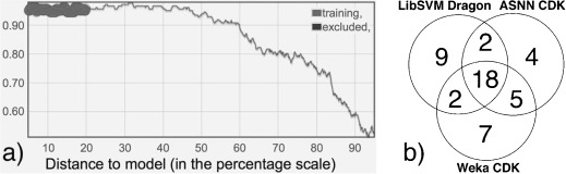
(a) Accuracy plot (y‐axis provides the ratio of correct predictions) for the WEKA model based on CDK descriptors with Bagging‐STD as distance to model. The 20 % of compounds with the lowest distance to the model, used for determination of outliers, are emphasized in the plot. (b) Venn diagram of the overlap of excluded compounds regarding 50 % of the lowest distance‐to‐model compounds (for the three best models of the whole dataset).

The models applying ASNN, Weka‐J48, Weka‐RF and LibSVM to CDK descriptors, Dragon6 descriptors, ISIDA fragments, and ALogPS/Estate indices were recalculated for the reduced dataset. Exclusion of the 48 compounds significantly improved the prediction accuracy. The BA of the recalculated models was over 86 %. On average, ASNN was the best performing method with averaged balanced accuracies of over 86 %. The differences in performance of the four methods were non‐significant. Regarding the descriptors, the CDK descriptor set resulted in the most accurate models, achieving averaged balanced accuracies of over 86 %. However, similar to the performances of machine learning algorithms, no significant differences in the performances of the four descriptor sets were observed.

3.2.5 Analysis of Excluded Compounds

The 48 excluded compounds comprised 25 and 23 substances that were NRB and RB, respectively. These outlier compounds were analyzed with respect to specific features that distinguished them from the correctly predicted compounds of the respective class. In order to do so, the OCHEM SetCompare tool was again used to identify characteristic features that were overrepresented in the respective sets of the excluded RB and NRB compounds.

We found that most outliers possessed characteristic features of the opposite class (i.e., outliers for the RB class had functional groups typical for NRB and vice versa). As shown in Table 4, many RB outlier compounds had aromatic substructures that were enriched within compounds of the NRB dataset (compare Table 1). Furthermore, the number of carboxylic acid derivatives, like carboxylic esters and carboxylic acids, was vanishingly small within the outlier compounds in the RB class, but larger in the NRB outlier class than expected from the analysis of the whole dataset: only 22 % of the RB outliers contained carboxylic acid moieties compared to 46 % of the >700 compounds in the RB dataset. In contrast, 52 % of the NRB outliers were composed of carboxylic acid derivatives, compared to 19 % of the original NRB dataset. The same applies for alcohols: there were no primary alcohols in the RB outlier class, but they occur more frequently than expected in the NRB outlier class (24 % compared to 6 % of original NRB class). And finally, compounds containing aliphatic chains were enriched in the NRB outlier class (32 % compared to 4 % of the original NRB class) but were absent in the RB outlier class (compared to 18 % in the original RB class).

Table 4.

The publisher did not receive permission from the copyright owner to include this object in this version of this product. Please refer either to the publisher's own online version of this product or the printed product where one exists.

In Table 5, four outlier compounds are given as illustration of the above results. The finding that outliers exhibit structural features of the opposite biodegradability class provides a convincing explanation for why these compounds were incorrectly predicted with high confidence by several models. We assume that some of the incorrectly predicted compounds were possibly experimental errors and thus their exclusion could contribute to the development of better models.

Table 5.

The publisher did not receive permission from the copyright owner to include this object in this version of this product. Please refer either to the publisher's own online version of this product or the printed product where one exists.

3.2.6 Analysis of 3D and 2D Descriptors

Since Dragon and CDK comprise a variety of descriptor subsets, it was interesting to examine whether subsets of 3D descriptors were important for the prediction of biodegradability of molecules. We identified descriptors that required 3D structures of molecules for Dragon and CDK and developed models with 3D and non‐3D subsets. The models based on non‐3D descriptors had similar accuracy to those based on the whole descriptor set.

3.2.7 Making Interpretable Models

While previous models achieved good accuracy, they could not be easily interpreted. Therefore, we developed a linear model using functional groups46 and the ALOGPS program48 as the interpretable descriptors.(3), (4)

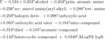(3)

(4)

Although the model BA is about 14 % lower than that of the models based on the aforementioned advanced machine learning methods, it allows a clear explanation of the results. Several of the structural features that were found to be significant in the structural analysis section are also present in the equation. For example, aromatic compounds and heterocyclic compounds, compounds with nitro, thiol, and amine groups, and halogenic derivatives determine low biodegradability (Y=0) of molecules. At the same time, the presence of alcohol, carboxylic acid, and acid ester groups increases the biodegradable potential of molecules.

3.2.8 Consensus Model

The consensus approach has been shown to provide models with a higher accuracy and coverage than the individual models.49–51 We developed a consensus model as a simple average of individual ASNN models, calculated for seven individual sets of descriptors. The ASNN models were selected since this method provided models with the highest accuracy on average. The new model had the same accuracy, a BA of 87.6 % ±1.6, and thus better statistical parameters than individual models. The consensus model obviously benefited from various representations of chemical structures, which characterized molecules from different perspectives. This model was selected as the final one and was used for further analyses reported in this article.

3.2.9 Predicting Molecules with Underrepresented Groups

The analysis using the ToxAlerts tool identified a number of functional groups that occurred only rarely in the training set. Molecules containing such groups could have a lower accuracy as these groups were underrepresented in the training set for model development. Indeed, we observed that the BA of the model for compounds containing groups that occurred five times or less (n=202 for 128 groups) in the training set was 0.84±0.06, but 0.88±0.02 for the remaining compounds. Thus, there was indeed some effect but the difference in BA values was not sufficiently large to state a statistically significant difference. The molecules with rare groups had a CONSENSUS‐STD=0.096 ±0.008, which was significantly higher than that calculated for the remaining compounds (0.081±0.03). Thus, the model differentiated both groups of compounds by indicating that molecules with rare groups were significantly more dissimilar (greater distance to model values) to the rest of the training set compounds.

3.2.10 Validation of the Model Using Test Sets

The validation protocol used in this study provided a so‐called “external” validation of all models. The term external, which is gaining some popularity in QSAR studies,17,52,53 is in our opinion a confusing one. Actually, there can be just two types of validation: “correct” or “biased.” The first, which is referred as “external,” tests a model following its development, i.e., following all model development steps including variable selection and parameter optimization. In our study, we always developed a new model for each fold, including parameter optimization, and only after that was the model used to predict a validation dataset. Thus, we indeed performed “external model validation” during each fold, and all reported cross‐validation results were thus “externally validated”.17,53 Typical examples of an incorrect validation procedure include either variable selection or tuning model parameters or both using all data, followed by a cross‐validation. Such an “internal” validation procedure can provide excellent statistical parameters using even random numbers, as was clearly demonstrated in one of our tutorials provided during the Summer Chemoinformatics School.54

We also decided to validate the performance of the model using two public test sets of 6355 and 40 (including 2 stereoisomers) compounds.25 The estimated average accuracy of the model of 83 % was in a good agreement with the calculated accuracy of 86±9 % for the Boethling and Costanza dataset.55 This result was better than the 75 % accuracy reported by the authors for their BIOWIN model.55 The consensus model identified seven predictions as outside the AD of the model and, in fact, failed to predict the correct biodegradability class for four of these. The consensus model provided very good results for NRB and only 4 out of 53 compounds from this class were incorrectly predicted. Unfortunately, the accuracy of the model was lower for RB compounds and 5 out of 10 compounds were incorrectly predicted. These five errors included three predictions marked as outside the AD of the model as well as theophylline and caffeine, i.e., two very similar compounds. This result is in accordance with other studies,7,14,56 which have consistently reported that prediction of biodegradable compounds is more challenging than predicting NRB ones. The consensus model correctly predicted all NRBs, but only 1 out of 3 RB compounds for the Steger‐Hartmann et al. set.25 Two incorrect predictions were testosterone and estradiol, which are naturally occurring sex hormones. The failure to correctly predict the biodegradability of these two compounds as well as that of theophylline and caffeine could be explained by acclimation of microbial communities to their exposure during evolution, i.e., the microbes may have developed very specialized pathways to degrade them. The Steger‐Hartmann et al. set25 contained about 10 further derivatives of the two steroid hormones, all of which were not biodegradable and thus correctly predicted by the model. Thus, even tiny modifications of the endogenous compounds can change their biodegradability. Dramatic differences in the biological properties of compounds due to minor variations in their structure are known as “activity cliffs” in drug discovery.57 Considering that the pharmaceutical industry invests hundreds of millions of dollars in the development of a single drug, but still faces the “activity cliffs” as one of its main challenges in drug discovery – for just one species, i.e., humans – it would be naïve to believe that a similar problem of “biodegradability cliffs” could easily be addressed in environmental studies. In this respect we cannot support the conclusion of Steger‐Hartmann et al., who stated that “based on the findings reported here, we consider the use of in silico tools for an early selection of drug candidates with favorable properties with regard to biodegradation as being currently immature.” In fact, with respect to the synthetic compounds, the consensus model gave a 100 % accurate prediction. In our view, because of differences in acclimation of microbial communities to synthetic and endogenous compounds and the aforementioned problem of “biodegradability cliffs,” the programs developed to predict the ready biodegradability of industrial compounds should not be tested using endogenous compounds.

From a formal viewpoint, the results of the consensus model were better than those of the BIOWIN model, which could not correctly predict three NRBs and failed to identify all RBs. However, due to the small size of these sets, the confidence intervals ranged from ±8 % to ±20 % for accuracy and balanced accuracy, respectively. Thus, when using such small sets, no statistically valid conclusion regarding higher performance of the current model can or should be drawn. We hope that registration of compounds in REACH will provide access to large number of experimental measurements, which can be used to provide large‐scale validation of existing approaches and the current model.

3.2.11 Screening of the ECHA Preliminary List of Chemical Compounds

The model was used to predict chemicals from ECHA’s preliminary list of chemical compounds pre‐registered for REACH, which was compiled at the Joint Research Center and is available as an Excel file for QSAR analysis.58 We applied the same filtering and exclusion of duplicated compounds as for the training set. Further, several other compounds, such as noble gasses, metals, and metal‐containing compounds were filtered, leaving 55 467 molecules. The consensus model predicted an average accuracy of 84.8 % for this dataset and about 87 % of the ECHA compounds were covered by its AD. The former percentage was calculated as the predicted average accuracy of the model for this set. The latter percentage does not mean that all 87 % of the predictions will be sufficient for regulatory purposes. The AD threshold used corresponded to an approximately 68 % probability of correct prediction, which could be low for some purposes. The consensus model covered 55 % and 43 % for thresholds of 80 % and 90 % predicted accuracy, respectively. Since the model always reports the prediction confidence, users can themselves decide whether the reported accuracy is sufficient for their purposes.

There were several functional groups calculated using ToxAlert (see Table S1 in the Supporting Information) for which many predictions of the consensus model were outside the AD and thus had low accuracy. For many of these groups, the training set contained only a few or even no training set samples. The average predicted accuracy of the model was RMSE=0.82 for groups represented by five or fewer compounds in the training set compared to RMSE=0.86 for the other groups. Thus, as previously reported for the training set, the model showed lower accuracy for these underrepresented groups. However, the accuracy of predictions for compounds within a group can show large variances. For example, there were only two compounds with a hexahydrotriazine group in the training set. Figure 2 shows four molecules with this group from the ECHA dataset. Molecule A, which is just the hexahydrotriazine core, was predicted as an NRB with lowest accuracy and marked as outside the AD of the model. Adding new groups increased the confidence of predictions for compounds B and C, which were predicted as NRB and RN. In the case of compound D, the addition did not change the accuracy of prediction; however, it changed its predicted class.

Figure 2.

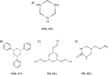
Biodegradability classes and the confidence of prediction as calculated by the consensus model for four compounds with a hexahydrotriazine group. The predictions for compounds A and D have the lowest accuracy and are flagged as outside the applicability domain of the model.

4 Discussion and Conclusions

We started with an initial dataset of ready biodegradability measurements for more than 2000 compounds, which was carefully cleaned and validated to provide a solid base for further analysis. Structural analysis of this dataset revealed that several characteristic functional groups were overrepresented in the two classes (RB and NRB). Whereas aromatic substructures and halogen derivatives are enriched in NRB compounds, carboxylic acid derivatives, alcohols, and aliphatic chains occur more frequently in RB compounds. The same result was confirmed by developing a linear model using the functional groups as descriptors.

From the initial dataset, several QSAR models were built for combinations of machine learning methods (ASNN, LibSVM, KNN, PLS, FSMLR, Weka‐J48, Weka‐RF) and descriptor sets (Dragon6, CDK, AlogPS, EState, Adriana, Chemaxon, ISIDA, GSFragments). This is thus the most comprehensive, up‐to‐date published study to predict the ready biodegradability of chemical compounds using different machine learning models and descriptor sets. The average balanced accuracy across all generated models was around 80 %, with some models achieving balanced accuracies of more than 84 %. This result suggests that there is no magic combination of methods and descriptors that appears preferably for the prediction of this property. The greatest accuracy was achieved using a consensus model, which averaged seven individual models: this thus highlights the importance of using different representations of chemical structures to obtain the most accurate predictor.

Stratified bagging with 64 bags was found to yield the best model performance: using a large number of bags did not increase the accuracy of the models. For the six best models, 48 outliers (2.5 % of all data points) were detected using Bagging‐STD (Figure 1). These outliers were incorrectly predicted with high confidence and therefore excluded from the dataset. Models derived with this reduced dataset showed an improved performance with a BA >86 %. Structural analysis of the outlier compounds revealed that they contained functional groups characteristic of the opposite biodegradability class (i.e., biodegradable outliers contained groups that were typically found in non‐biodegradable compounds, and vice versa). That is why these molecules were incorrectly classified despite the high accuracy of prediction reported by the models. It is possible that their reported biodegradability classes were experimental errors and/or the compounds were measured in inappropriate experimental settings.

Models generated with 2D subsets of the Dragon6 and CDK descriptors showed that 2D features were sufficient to yield models with a similar accuracy to those built using the whole sets of descriptors. Thus, 2D characteristics such as the occurrence of certain functional groups could be sufficient to provide a prediction of biodegradability.

The proposed workflow for data analysis and identification of outlying compounds provides an important methodological development to identify and exclude erroneous data and significantly improve model accuracy.

The approach used in this study was somewhat different to previously published studies. In general, previous authors identify some set of the most important descriptors, i.e., molecular fragments, which are then used to develop the models. In addition, identification of such fragments is used to provide an interpretation of the models. However, if such models are applied to new compounds, a lower prediction performance is reported, quite often due to the missing “fragments” problem.5 Therefore, in the current study we explored a different approach: no descriptor selection (except for filtering highly correlated descriptors) was used and thus models were developed using all available structural information. The prediction of individual models was then used to develop a final consensus model. In our view, a model developed in this way is more robust and better able to predict new chemical structures. Indeed, thanks to the different representations of chemical structures used in the individual models, the consensus model is more easily able to account for new chemical substructures. The future benchmarking of the model for new datasets will allow this hypothesis to be tested.

Application of the developed models to predict two test sets resulted in similar performances to previous models. We showed that the accuracy and BA calculated for both test sets had very wide confidence intervals, which were estimated using a bootstrap procedure. Therefore, they were making an infeasible comparison of different models using these sets. This result is an important warning to users who frequently ignore the variance of statistical coefficients when comparing the performance of models. Conclusions based on such comparisons could be incorrect simply due to chance effects.

In summary, in this study our aim was twofold: (i) to develop a consensus model to predict the ready biodegradability of chemical compounds, and (ii) to make this model publicly available. This is the first publicly available consensus model for ready biodegradability based on seven individual models and using the largest dataset. In contrast to previous models, the new model provides confidence intervals for each prediction. This allows the final user to decide whether the provided accuracy of prediction is satisfactory or whether experimental measurement is required. The strategy of identifying and excluding outlying molecules, as described in the article, provides an important methodological approach for working with noisy data. We also suggested that model developers should take the confidence intervals of statistical parameters into account. This is crucial in order to avoid erroneous conclusions when comparing model performances. Finally, we discussed why the testing of models developed using industrial chemicals could be biased when using endogenous compounds. Such compounds could have a higher biodegradability potential due to acclimation of microbial communities, leading to “biodegradability cliffs.” The public availability of our model and all its data will allow other users to validate its results. It will also contribute to its promotion59 and a wider use of computational methods in the environmental sciences.

Conflict of Interest

Dr. Igor V. Tetko is the founder of eADMET GmbH, which licenses the OCHEM software.

Supporting information

As a service to our authors and readers, this journal provides supporting information supplied by the authors. Such materials are peer reviewed and may be re‐organized for online delivery, but are not copy‐edited or typeset. Technical support issues arising from supporting information (other than missing files) should be addressed to the authors.

miscellaneous_information

si_tables

References

- 1. Struijs J., Stoltenkamp J., Sci. Total. Environ. 1986, 57, 161–170. [DOI] [PubMed] [Google Scholar]
- 2. Carson D. B., Saege V. W., Gledhill W. E., in Aquatic Toxicology Risk Assessment, Vol. 13, ASTM STP 1096, 1990, pp. 48–59. [Google Scholar]
- 3.OECD, Test No. 301: Ready Biodegradability, 1992, http://dx.doi.org/10.1787/9789264070349‐en.
- 4.OECD, Detailed Review Paper on Biodegradability Testing, 2002, http://dx.doi.org/10.1787/9789264078529‐en.
- 5. Pavan M., Worth A. P., QSAR Comb. Sci. 2008, 27, 32–40. [Google Scholar]
- 6. Rücker C., Kümmerer K., Green Chem. 2012, 14, 875–887. [Google Scholar]
- 7. Jaworska J. S., Boethling R. S., Howard P. H., Environ. Toxicol. Chem. 2003, 22, 1710–1723. [DOI] [PubMed] [Google Scholar]
- 8. Howard P. H., Boethling R. S., Stiteler W., Meylan W., Beauman J., Sci. Total. Environ. 1991, 109–110, 635–641. [DOI] [PubMed] [Google Scholar]
- 9. Klopman G., Quant. Struct. Act. Relat. 1992, 11, 176–184. [Google Scholar]
- 10. Loonen H., Lindgren F., Hansen B., Karcher W., Niemelä J., Hiromatsu K., Takatsuki M., Peijnenburg W., Rorije E., Struijś J., Environ. Toxicol. Chem. 1999, 18, 1763–1768. [Google Scholar]
- 11. Gamberger D., Horvatić D., Sekušak S., Sabljić A., Environ. Sci. Pollut. Res. 1996, 3, 224–228. [DOI] [PubMed] [Google Scholar]
- 12. Boethling R. S., Howard P. H., Meylan W., Stiteler W., Beauman J., Tirado N., Environ. Sci. Technol. 1994, 28, 459–465. [DOI] [PubMed] [Google Scholar]
- 13. Klopman G., Tu M., Environ. Toxicol. Chem. 1997, 16, 1829–1835. [Google Scholar]
- 14. Sakuratani Y., Yamada J., Kasai K., Noguchi Y., Nishihara T., SAR QSAR Environ. Res. 2005, 16, 403–431. [DOI] [PubMed] [Google Scholar]
- 15. Gao J., Ellis L. B., Wackett L. P., Nucleic Acids Res. 2011, 39, W406–411. [DOI] [PMC free article] [PubMed] [Google Scholar]
- 16. Eriksson L., Jaworska J., Worth A. P., Cronin M. T., McDowell R. M., Gramatica P., Environ. Health Perspect. 2003, 111, 1361–1375. [DOI] [PMC free article] [PubMed] [Google Scholar]
- 17. Tetko I. V., Sushko I., Pandey A. K., Zhu H., Tropsha A., Papa E., Oberg T., Todeschini R., Fourches D., Varnek A., J. Chem. Inf. Model. 2008, 48, 1733–1746. [DOI] [PubMed] [Google Scholar]
- 18. Sushko I., Novotarskyi S., Korner R., Pandey A. K., Cherkasov A., Li J., Gramatica P., Hansen K., Schroeter T., Muller K. R., Xi L., Liu H., Yao X., Oberg T., Hormozdiari F., Dao P., Sahinalp C., Todeschini R., Polishchuk P., Artemenko A., Kuz′min V., Martin T. M., Young D. M., Fourches D., Muratov E., Tropsha A., Baskin I., Horvath D., Marcou G., Muller C., Varnek A., Prokopenko V. V., Tetko I. V., J. Chem. Inf. Model. 2010, 50, 2094–2111. [DOI] [PubMed] [Google Scholar]
- 19. Kirkpatrick P., Ellis C., Nature 2004, 432, 823–823. [Google Scholar]
- 20.I. Sushko, S. Novotarskyi, R. Korner, A. K. Pandey, M. Rupp, W. Teetz, S. Brandmaier, A. Abdelaziz, V. V. Prokopenko, V. Y. Tanchuk, R. Todeschini, A. Varnek, G. Marcou, P. Ertl, V. Potemkin, M. Grishina, J. Gasteiger, C. Schwab, J. J. Baskin, V. A. Palyulin, E. V. Radchenko, W. J. Welsh, V. Kholodovych, D. Chekmarev, A. Cherkasov, J. Aires‐de‐Sousa, Q. Y. Zhang, A. Bender, F. Nigsch, L. Patiny, A. Williams, V. Tkachenko, I. V. Tetko, J. Comput. Aided. Mol. Des. 2011, 25, 533–554. [DOI] [PMC free article] [PubMed]
- 21. Cheng F., Ikenaga Y., Zhou Y., Yu Y., Li W., Shen J., Du Z., Chen L., Xu C., Liu G., Lee P. W., Tang Y., J. Chem. Inf. Model. 2012, 52, 655–669. [DOI] [PubMed] [Google Scholar]
- 22. Tunkel J., Howard P. H., Boethling R. S., Stiteler W., Loonen H., Environ. Toxicol. Chem. 2000, 19, 2478–2485. [Google Scholar]
- 23. Oprisiu I., Novotarskyi S., Tetko I. V., J. Cheminform. 2013, 5, 4. [DOI] [PMC free article] [PubMed] [Google Scholar]
- 24. Boethling R. S., Howard P. H., Meylan W. M., Environ. Toxicol. Chem. 2004, 23, 2290–2308. [DOI] [PubMed] [Google Scholar]
- 25. Steger‐Hartmann T., Lange R., Heuck K., Environ. Sci. Pollut. Res. Int. 2011, 18, 610–619. [DOI] [PubMed] [Google Scholar]
- 26. Tetko I. V., Neur. Proc. Lett. 2002, 16, 187–199. [Google Scholar]
- 27. Tollenaere T., Neural Netw. 1990, 3, 561–573. [Google Scholar]
- 28. Zhokhova N. I., Baskin I. I., Palyulin V. A., Zefirov A. N., Zefirov N. S., Dokl. Chem. 2007, 417, 282–284. [Google Scholar]
- 29.C.‐C. Chang, C.‐J. Lin, ACM Trans. Intell. Syst. Technol. 2011, 2, 27 : 21–27 : 27.
- 30.J. R. Quinlan, C4.5: Programs for Machine Learning, Morgan Kaufmann, San Francisco, CA, USA, 1993.
- 31. Hall M., Frank E., Holmes G., Pfahringer B., Reutemann P., Witten I. H., SIGKDD Explorations 2009, 11. [Google Scholar]
- 32. Breiman L., Machine Learn. 2001, 45, 5–32. [Google Scholar]
- 33. Sadowski J., Gasteiger J., Klebe G., J. Chem. Inf. Comput. Sci. 1994, 34, 1000–1008. [Google Scholar]
- 34. Hall L. H., Kier L. B., J. Chem. Inf. Comput. Sci. 1995, 35, 1039–1045. [Google Scholar]
- 35. Tetko I. V., Tanchuk V. Y., J. Chem. Inf. Comput. Sci. 2002, 42, 1136–1145. [DOI] [PubMed] [Google Scholar]
- 36. Tetko I. V., Tanchuk V. Y., Villa A. E., J. Chem. Inf. Comput. Sci. 2001, 41, 1407–1421. [DOI] [PubMed] [Google Scholar]
- 37. Varnek A., Fourches D., Horvath D., Klimchuk O., Gaudin C., Vayer P., Solov′ev V., Hoonakker F., Tetko I. V., Marcou G., Curr. Comput.‐Aided Drug Des. 2008, 4, 191–198. [Google Scholar]
- 38. Stankevich I. V., Skvortsova M. I., Baskin I. I., Skvortsov L. A., Palyulin V. A., Zefirov N. S., J. Mol. Struct. 1999, 466, 211–217. [Google Scholar]
- 39. Steinbeck C., Han Y., Kuhn S., Horlacher O., Luttmann E., Willighagen E., J. Chem. Inf. Comput. Sci. 2003, 43, 493–500. [DOI] [PMC free article] [PubMed] [Google Scholar]
- 40. Todeschini R., Consonni V., Handbook of Molecular Descriptors, WILEY‐VCH, Weinheim, 2000. [Google Scholar]
- 41. Gasteiger J., J. Med. Chem. 2006, 49, 6429–6434. [DOI] [PubMed] [Google Scholar]
- 42. Breiman L., Machine Learn. 1996, 24, 123–140. [Google Scholar]
- 43. Kotsiantis S. B., Kanellopoulos D., Pintelas P. E., Int. Trans. Comp. Sci. Eng. 2006, 30, 25–36. [Google Scholar]
- 44. Brodersen K. H., Ong C. S., Stephan K. E., Buhmann J. M., Proc. 20th Int. Conf. Pattern Recognition 2010, pp. 3121–3124. [Google Scholar]
- 45. Sushko I., Salmina E., Potemkin V. A., Poda G., Tetko I. V., J. Chem. Inf. Model. 2012, 52, 2310–2316. [DOI] [PMC free article] [PubMed] [Google Scholar]
- 46. Haider N., Molecules 2010, 15, 5079–5092. [DOI] [PMC free article] [PubMed] [Google Scholar]
- 47. Fromel T., Knepper T. P., Rev. Environ. Contam. Toxicol. 2010, 208, 161–177. [DOI] [PubMed] [Google Scholar]
- 48. Tetko I. V., Tanchuk V. Y., Kasheva T. N., Villa A. E., J. Chem. Inf. Comput. Sci. 2001, 41, 1488–1493. [DOI] [PubMed] [Google Scholar]
- 49. Zhu H., Tropsha A., Fourches D., Varnek A., Papa E., Gramatica P., Oberg T., Dao P., Cherkasov A., Tetko I. V., J. Chem. Inf. Model. 2008, 48, 766–784. [DOI] [PubMed] [Google Scholar]
- 50.I. V. Tetko, S. Novotarskyi, I. Sushko, V. Ivanov, A. E. Petrenko, R. Dieden, F. Lebon, B. Mathieu, J. Chem. Inf. Model. 2013, 53, 1990–2000. [DOI] [PMC free article] [PubMed] [Google Scholar]
- 51. Cassani S., Kovarich S., Papa E., Roy P. P., Rahmberg M., Nilsson S., Sahlin U., Jeliazkova N., Kochev N., Pukalov O., Tetko I., Brandmaier S., Durjava M. K., Kolar B., Peijnenburg W., Gramatica P., ATLA: Altern. Lab. Anim. 2013, 41, 49–64. [DOI] [PubMed] [Google Scholar]
- 52. Tropsha A., Mol. Inf. 2010, 29, 476–488. [DOI] [PubMed] [Google Scholar]
- 53. Tetko I. V., Solov′ev V. P., Antonov A. V., Yao X., Doucet J. P., Fan B., Hoonakker F., Fourches D., Jost P., Lachiche N., Varnek A., J. Chem. Inf. Model. 2006, 46, 808–819. [DOI] [PubMed] [Google Scholar]
- 54. Tetko I. V., Baskin I. I., Varnek A., in Strasbourg Summer School on Chemoinformatics: CheminfoS3 Obernai, 2008. [Google Scholar]
- 55. Boethling R. S., Costanza J., SAR QSAR Environ. Res. 2010, 21, 415–443. [DOI] [PubMed] [Google Scholar]
- 56. Rorije E., Loonen H., Muller M., Klopman G., Peijnenburg W. J., Chemosphere 1999, 38, 1409–1417. [DOI] [PubMed] [Google Scholar]
- 57. Maggiora G. M., J. Chem. Inf. Model. 2006, 46, 1535. [DOI] [PubMed] [Google Scholar]
- 58.EINECS list processed file for QSAR analysis, 2009, http://ihcp.jrc.ec.europa.eu/our_labs/predictive_toxicology/information‐sources/ec_inventory.
- 59. Tetko I. V., J. Comput. Aided. Mol. Des. 2012, 26, 135–136. [DOI] [PubMed] [Google Scholar]
Associated Data
This section collects any data citations, data availability statements, or supplementary materials included in this article.
Supplementary Materials