NanoStringDiff: a novel statistical method for differential expression analysis based on NanoString nCounter data

Abstract

The advanced medium-throughput NanoString nCounter technology has been increasingly used for mRNA or miRNA differential expression (DE) studies due to its advantages including direct measurement of molecule expression levels without amplification, digital readout and superior applicability to formalin fixed paraffin embedded samples. However, the analysis of nCounter data is hampered because most methods developed are based on t-tests, which do not fit the count data generated by the NanoString nCounter system. Furthermore, data normalization procedures of current methods are either not suitable for counts or not specific for NanoString nCounter data. We develop a novel DE detection method based on NanoString nCounter data. The method, named NanoStringDiff, considers a generalized linear model of the negative binomial family to characterize count data and allows for multifactor design. Data normalization is incorporated in the model framework through data normalization parameters, which are estimated from positive controls, negative controls and housekeeping genes embedded in the nCounter system. We propose an empirical Bayes shrinkage approach to estimate the dispersion parameter in the model and a likelihood ratio test to identify differentially expressed genes. Simulations and real data analysis demonstrate that the proposed method performs better than existing methods.

INTRODUCTION

The NanoString nCounter system provides a simple and cost-effective way to profile specific nucleic acid molecules in a complex mixture. The system uses target-specific color-coded barcodes that can hybridize directly to target molecules. The expression level of a target molecule is measured by counting the number of times the barcode for that molecule is detected by a digital analyzer. The system does not need amplification and is sensitive enough to detect low abundance molecules (1). It can simultaneously quantify up to 800 different interesting targets, making it ideal for miRNA profiling and targeted mRNA expression analysis. The NanoString nCounter system also provides more accurate quantifications of mRNA expressions than polymerase chain reaction (PCR)-based methods and microarrays in formalin fixed paraffin embedded samples, where RNA degradation is commonly observed (2).

One of the fundamental tasks for molecule expression studies is to identify differential expression (DE) for mRNAs or miRNAs across experimental conditions. We use genes thereafter for convenience. Most current methods for DE detection in nCounter data, such as NanoStringNorm (3) and NanoStriDE (4), are based on t-tests. Although popular, the t-test is most appropriate for analyzing continuous, preferably normally distributed data. However, data produced by nCounter Analyzer are counts. Therefore, it is more natural to use a discrete distribution to characterize the data. Brumbaugh et al. (4) suggested the use of DESeq (5), a tool developed for RNA-seq, to analyze nCounter data because the method uses a negative binomial model for count data from RNA-seq. However, nCounter data and RNA-seq data are different, especially in data normalization, as we discuss in the following paragraph. To our knowledge, there has not been a discrete statistical model specifically designed for nCounter data.

Data normalization is a crucial step for using nCounter to quantify gene expression. The nCounter platform provides positive controls, housekeeping genes, and negative controls to quantify lane-specific variation, differences in sample input, and non-specific background, respectively. A common data normalization procedure includes dividing the raw data by size factors and subtracting background level (3,4). This procedure, however, spoils the discrete nature of the data and makes them ineligible to be analyzed as counts. As an alternative approach, methods developed for RNA-seq data analysis, e.g. DESeq and edgeR (6–8), treated the size factor as a scaling parameter in the negative binomial model for data normalization. However, since those methods were developed for RNA-seq, they did not utilize positive controls and housekeeping genes when calculating the size factor. They also did not adjust for background noise, which can lead to biased quantification of gene expression, especially when the expression level is relatively low. Therefore, the results of normalization based on them may be less than optimal.

In this paper, we present a novel DE detection method specifically designed for nCounter data, which fully takes into account the discrete nature of the data and the critical need for data normalization. Our method, named NanoStringDiff, utilizes a generalized linear model (GLM) of the negative binomial family to characterize count data and allows for multi-factor design. We incorporate size factors, calculated from positive controls, housekeeping genes and background level, obtained from negative controls, in the model framework, so that all the normalization information provided by nCounter Analyzer is fully utilized. As demonstrated by simulations and real data analysis, our method provides more accurate and powerful results in DE detection compared to existing methods.

MATERIALS AND METHODS

Normalization parameters

Data generated by the nCounter system have to be normalized prior to being used to quantify gene expression and compare expression rate between different experimental conditions. Data normalization includes adjustment for sample preparation variation, background noise and sample content variation. We introduce three normalization parameters to quantify these variations and noise, respectively. These parameters can be directly informed from the internal controls of the nCounter system.

Positive control size factor (c_i): this size factor accounts for lane-by-lane variation. The nCounter Analyzer has six spike-in positive hybridization controls with different concentrations for each sample, which can be used to infer c_i.

Background noise parameter (θ_i): this parameter quantifies the non-specific background level. The nCounter Analyzer includes six to eight negatives control probes that have no target in the sample. The observed expression levels of those negative controls characterize θ_i.

Housekeeping size factor (d_i): this size factor adjusts for the variation in the amount of input sample material. The nCounter system suggests the use of housekeeping genes, whose expressions are stable across samples, to inform this factor. NanoString provides a variety of housekeeping genes for users to choose from. Typically, at least three housekeeping genes are included in the CodeSet.

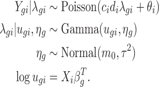
The data model

Denote the observed count from gene g in sample i by Y_gi, and the unobserved expression rate by λ_gi. We assume a Poisson model for Y_gi given λ_gi:

Our model incorporates the positive control size factor, c_i and the housekeeping size factor, d_i, to adjust for the sample-by-sample difference due to experimental variations. It also includes the background noise parameter, θ_i, to adjust for non-specific background. Using the additive property of the Poisson distribution, we can decompose Y_gi into Z_gi + B_gi, where Z_gi|λ_gi ∼ Poisson(c_id_iλ_gi) denotes the count from the expression of gene g and B_gi ∼ Poisson(θ_i) denotes the background noise.

Due to biological variation, expression rates among samples from the same treatment group are not identical. This results in the over-dispersion problem, where the observed variation is larger than expected by the Poisson model. This problem is well recognized in RNA-seq experiments, where the data are also in counts (5,6). A common approach to address the problem is to consider a Bayesian hierarchical model, where a Gamma distribution is used to characterize the variation in the underlying expression rate:

Here the Gamma distribution is parameterized with mean u_gi and log dispersion η_g, where η_g is the negative of logarithm of the shape parameter in the common parameterization. Let v_gi = c_id_iu_gi, then based on the hierarchical model, the marginal distribution of Z_gi given v_gi and η_g is negative binomial with mean v_gi and variance 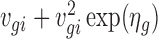. Therefore, the marginal distribution of Y_gi is the convolution of a negative binomial distribution and a Poisson distribution.

Consider a general, multifactor experiment. Let X be the design matrix, where the number of rows is the number of samples and the number of columns is the number of covariates. The mean parameter u_gi is specified based on a GLM with logarithmic link function:

where X_i represents the ith row of the design matrix X, which is a vector of covariates that specifies the treatment conditions applied to sample i, and β_g is a vector of regression coefficients quantifying the covariates effects for gene g. The DE analysis for experimental factor j can be performed by evaluating the hypothesis H₀: β_gj = 0, where β_gj is the jth element of β_g.

Accurate estimation of the dispersion parameter plays an important role in DE detection and shrinkage estimators have been shown to be useful in typical RNA-seq experiments when the number of replicates is small (5,8–10). Because the nCounter data is most similar to the RNA-seq data in the aspects of data discreteness and very limited number of replicates, we borrow the shrinkage method developed for RNA-seq data to estimate the dispersion parameter. Specifically, we consider an empirical Bayes shrinkage method (10), which introduces a prior distribution for the dispersion parameter and borrows information from the ensemble of genes to estimate the dispersion parameter for a specific gene. Supplementary Figure S1 depicts the empirical distribution of log dispersion η_g for several real datasets. Those histograms show that η_g can be approximately modeled by a normal distribution. Thus, we consider the following prior:

where m₀ and τ² are hyper-parameters representing mean and variance for the normal distribution, respectively.

To sum up, the hierarchical model we consider is as follows:

(1)

Parameter estimation and differential expression analysis

Estimating size factors and background noise

Appropriate estimation of the positive control size factor, background noise parameter and housekeeping size factor can effectively improve the accuracy of DE detection. The nCounter system suggests using the spike-in positive and negative control genes to estimate positive size factor and background noise. For each sample, nCounter provides six positive controls corresponding to six different concentrations in the 30 µl hybridzation: 128, 32, 8, 2, 0.5 and 0.125fM. It also provides six to eight negative controls, which can be seen as corresponding to 0fM, as no transcript is expected. We consider a Poisson model for those spike-in control genes. For each sample i, let M_gi denote the read count for spike-in control gene g, θ_i denote the sample-specific background noise, q_i denote the expression rate and con_g denote the concentration for spike-in control gene g, we assume:

By fitting the Poisson model, we obtain the maximum likelihood estimates (MLEs) and . Then the background noise parameter can be estimated by , and the positive size factor can be estimated by

where n is the number of samples.

The housekeeping size factor can be estimated from housekeeping genes. Because the expressions of housekeeping genes are also affected by platform source of variation and background noise, we standardize the observed read counts for housekeeping genes, H_gi, as follows:

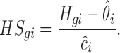Then we calculate the ratio of HS_gi for sample i relative to its average across all samples and use the median of the ratios for all housekeeping genes as the estimate of the housekeeping size factor. Mathematically,

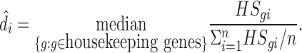Estimating hyper-parameters for the distribution of the dispersion parameter

The hyper-parameters are empirically estimated using expression data for endogenous genes (i.e. the target genes). Specifically, for each endogenous gene, we get the MLE of the log dispersion parameter, denoted by . Because data contain background noise and endogenous genes with very low read counts cannot provide effective information, we only use from endogenous genes with read counts larger than the the maximum value of negative controls to estimate the hyper-parameters. We use the median of for those endogenous genes to estimate m₀, i.e. . The estimation of τ² is more complex. As pointed out by Wu et al. (10), , where is the variation due to estimating η_g. Therefore, the sample variance of overestimates τ². Similar to Wu et al. (10), we first use an ad hoc method to create some pseudo datasets with τ² = 0 to estimate , then subtract it from the sample variance of to obtain an estimate of τ².

Estimating model coefficients and dispersion

The marginal probability mass function for Y_gi can be derived as (see Supplementary Data, Section 1 for details):

where 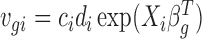. We estimate β_g and η_g using an iterative procedure. To estimate β_g, we consider its likelihood function for a given η_g:

(2)

and obtain the MLE, . To estimate η_g, we consider its posterior distribution given Y_gi and β_g, p(η_g|Y_gi, β_g, i = 1, ..., n), which satisfies

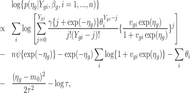(3)

where ψ(.) is the log gamma function. The derivation of this formula is provided in Supplementary Data, Section 2. Equation (3) also can be viewed as a penalized log likelihood function with penalty , penalizing values that deviate far from the common prior m₀. Estimates of size factors, background noise and hyper-parameters are plugged into Equation (3) and treated as constants. For a given β_g, we obtain the estimate of η_g, denoted by , by maximizing Equation (3).

We start with as the initial value of η_g, plug it into Equation (2) to obtain . Then we plug into Equation (3) to obtain . By iteratively updating and until convergence, we obtain estimates for β_g and η_g.

Hypothesis testing and false discovery rate

We consider a likelihood ratio test for DE detection. For each gene, we compare the maximum of the log of the likelihood in Equation (2) under the null hypothesis versus that without any constraint. The chi-square approximation is used to obtain a P-value. The Benjamini and Hochberg procedure(11) is used to calculation the false discovery rate (FDR).

Q-PCR validation of miRNAs

Total RNA was extracted using TRizol reagent (Life Technologies, Grand Island, NY, USA). For miRNA including internal control U6, the single-stranded cDNA from total RNA (20 ng) was synthesized using specific miRNA primers from the TaqMan MicroRNA Assays and reagents from the TaqMan MicroRNA Reverse Transcription (RT) Kit according to the manufacture's instruction. For β-actin and 18S internal controls, cDNA was prepared from the total RNA using the High Capacity cDNA Reverse Transcription Kit (Life Technologies). Expression of target genes was then assessed by Comparative Ct (ΔΔCt) using commercially available probes and TaqMan Universal PCR master mix and performed on a StepOnePlusTM 96-well instrument as described by the manufacturer (Life Technologies). The expression level of each miRNA targets was normalized by β-actin, 18S or U6 RNA and reported as a relative level to a specified control, as noted. The data were analyzed by two-sample t-tests.

RESULTS

Data description

The following four real nCounter datasets were used to generate simulation studies to evaluate the performance of our proposed method.

Horbinski data

Horbinski et al. studied human glioma cell lines expressing GFP or GFP with IDH1 mutation (R132H) (GSE80821). The cells were grown in vitro for 6 days. Eight hundred miRNAs were profiled with three replicates in each group. The data for the mutant group were used in this paper.

Mori data

Mori et al. (12) studied the possible reasons responsible for the widespread miRNA repression observed in cancer, global microRNA expression in mouse liver normal tissues and liver tumors induced by deletion of Nf2 (merlin) were profiled by nCounter Mouse miRNA Expression Assays (GSE52207). Expressions of 599 miRNAs were measured with two replicates in each group. The data for the normal group were used in this paper.

Busskamp data

Busskamp et al. (13) profiled miRNAs of iPS cells (PGP1) at 0, 1, 3 and 4 days post-doxycycline induction of murine NGN1 and NGN2 using the nCounter human miRNA assay kit v1 (GSE62145). Expressions of 734 miRNAs were profiled for three replicates in each group. The data for day 3 were used in this paper.

Teruel-Montoya data

Teruel-Montoya et al. (14) used the nCounter human miRNA assay kit v1 and v2 to profile miRNAs in normal human platelets, T-cells, B-cells, granulocytes and erythrocytes from five healthy male donors (GSE57679). The data for B-cells were used in this paper, where expressions of 730 miRNAs were profiled with five replicates in the B-cell group.

In addition, as a real data analysis, we applied our method to identify differentially expressed miRNAs between the mutant and GFP control groups for the Horbinski data.

Simulations

We performed comprehensive simulation studies to evaluate the performance of our NanoStringDiff method and to compare with two other software packages that have been proposed for analyzing NanoString data (3,4): NanoStringNorm (version 1.1.21) and DESeq2 (version 1.10.0). For NanoStringNorm, we called function NanoStringNorm with one recommended setting, that is using geometric mean to estimate positive size factor and housekeeping size factor and using mean background value plus two standard deviation as background threshold. For DESeq2, we called the function DESeq with default settings. The DESeq method (5) was originally developed for RNA-seq data and had been suggested to analyze NanoString data by Brumbaugh et al. (4). Here, we considered its successor, DESeq2 (15), in the methods comparison. To more generally assess the difference between NanoStringDiff and RNA-seq data analysis methods, we also compared our method to edgeR (version 3.12.0) (6–8), which is another frequently used method for RNA-seq data analysis.

To evaluate DE detection under known truth, and to conduct the comparison under realistic scenarios encountered in nCounter experiments, data were generated based on model (1) using parameters estimated from the four real datasets described above. The results for using parameters from Horbinski data and Mori data are provided in this section and those for using parameters from the other two datasets are provided in Supplementary Data. All simulations were for two-group comparison evaluating 800 candidate endogenous genes with 150 being true differentially expressed. The mean expression parameter λ_gi was randomly re-sampled from the means calculated from the real datasets. For DE genes, the log fold change was generated randomly from a mixture distribution 0.5N(1, 0.3) + 0.5N(−1, 0.3). The log dispersion parameter η_g was simulated based on two different methods: (i) generated from a normal distribution, with parameters computed from the real datasets; and (ii) re-sampled from the dispersions calculated using the real datasets. We present in this section the results for using a normal distribution to generate the dispersion parameter. The results for using the other method to generate the dispersion parameter are provided in Supplementary Data, Section 9. For each simulation scenario, we considered three, five or eight replicates in each treatment group and ran 100 simulations. A detailed description of simulation settings is provided in Supplementary Data, Section 4.

We first evaluated the estimation of size factors based on NanoStringDiff, and compared to DESeq2 and edgeR. Figure 1A–C plot the NanoString estimated positive size factor, housekeeping size factor and sample specific background noise against their true values, respectively. NanoStringDiff provides accurate estimation of those parameters. For comparison with DESeq2 and edgeR, we define an overall size factor as the product of the positive size factor and the housekeeping size factor. The overall size factor is used in DESeq2 and edgeR, where it is estimated by using data from endogenous genes. Figure 1D plots the estimated overall size factor against the true value based on NanoStringDiff, DESeq2 and edgeR. The overall size factor estimated from NanoStringDiff has a much smaller variation compared to DESeq2 and edgeR. This is because NanoStringDiff fully utilizes the positive controls and housekeeping genes information provided by nCounter to estimate the size factor. In contrast, such information is not used by DESeq2 and edgeR.

Figure 1.

Estimation of normalization parameters. (A) Positive size factor estimated from NanoStringDiff against its true value; (B) Housekeeping size factor estimated from NanoStringDiff against its true value; (C) Background noise estimated from NanoStringDiff against its true value; (D) The overall size factor estimated from NanoStringDiff, DESeq2 and edgeR against its true value; For NanoStringDiff, the estimated overall size factor was the product of the estimated positive and housekeeping size factors; For DESeq2 and edgeR: the estimated overall size factor was directly calculated from the algorithm. Results were from a dataset simulated based on the Horbinski data with three replicates and averaged across the replicates.

We next assessed the control of type I error rate for the likelihood ratio test in NanoStringDiff. Supplementary Figure S3 plots the reported type I error rate against the true type I error rate based on simulated data. For data simulated based on Horbinski data and Mori data, our method provided good control of the type I error rate: the reported value was close to the true value. But for some other simulation scenarios, the type I error rate was inflated. A more comprehensive evaluation of this issue is provided in the ‘Discussion’ section and Supplementary Data, Section 6.

An important task of DE analysis is to rank genes based on their evidence of being differentially expressed. From this point of view, the ability to have as many true positives as possible in the top-ranked genes is a critical part of evaluating the performance of a method. We compared the receiver operating characteristic (ROC) curve, which shows true positive rate and false positive rate at various thresholds, among NanoStringDiff, NanoStringNorm, DESeq2 and edgeR (Figure 2). Note that we only used genes having at least one average expression count after adjusting background noise because there was no classification power for genes with average count lower than background noise (area under the ROC curve (AUC) close to 0.5 for all three methods, data not shown). Separate ROC curves were generated for genes with average count, after adjusting background noise, between 1 and 100, and higher than 100. For genes with average count between 1 and 100, ROC curves from NanoStringDiff were higher than those for DESeq2 and NanoStringNorm, indicating better performance of NanoStringDiff in providing higher true positive rates at given false positive rates. The ROC curves from NanoStringDiff and edgeR were close to each other. For genes with average count larger than 100, as expected, the ROC curves were higher for all methods. The difference across methods were also much smaller due to the less impact of background noise adjustment at large read counts.

Figure 2.

ROC curves comparing different methods. Separate curves were generated for genes with average read count after adjusting background noise between 1 and 100 (left column), and higher than 100 (right column). Results were from data simulated based on Horbinski Data (first row) and Mori Data (second row) with three replicates.

In practice, DE genes are often declared based on a user-specified FDR threshold. Given the threshold, a powerful method is expected to identify as many true DE genes as possible. We compared the number of DE genes identified under a given FDR threshold (0.05, 0.1 or 0.2) among different methods. As shown in Figure 3, NanoStringDiff detected more true DE genes than NanoStringNorm, DESeq2 and edgeR.

Figure 3.

Bar charts for number of positive calls under a given FDR threshold comparing different methods. Results were averaged across 100 datasets simulated based on the Horbinski data (left column) and Mori data (right column) with three, five or eight replicates. For each simulation scenario, three different FDR thresholds, 0.05, 0.1 and 0.2, were considered. The shaded area represents false discoveries, i.e. the number of non-DE genes within positive calls.

We also investigated the control of FDR for different methods. Figure 4 plots the reported FDR against the true FDR for each method. The reported FDR curves from NanoStringDiff were close to true FDR curves. In contrast, the true FDR from NanoStringNorm and DESeq2 were much smaller than the reported FDR. The true FDR from edgeR was also much smaller than the reported FDR in most cases. Therefore, those methods were over conservative, which partially explains the limited number of true DE genes they could identify for a given FDR threshold.

Figure 4.

FDR estimation comparing different methods. Results were averaged across 100 datasets simulated based on Horbinski data (left column) and Mori data (right column) with three, five or eight replicates.

Real data analysis

We applied NanoStringDiff to the Horbinski data to identify miRNAs differentially expressed between IDH1 mutant and GFP control. For methods comparison, we also considered NanoStringNorm, DESeq2, edgeR and NanoStriDE (4), which is an online application to perform DE analysis for NanoString nCounter data. NanoStriDE provides two options: DESeq and t-test. We considered both options with their default settings in our analysis. Choosing 0.01 as the FDR threshold, NanoStringDiff identified 14 DE miRNAs, which are listed in Table 1. In contrast, DESeq2 only identified 2 DE miRNAs (indicated by * in Table 1), both edgeR and NanaStriDE with the DESeq option only identified 1 DE miRNA (indicated by ⁺ in Table 1), neither NanoStringNorm nor NanoStriDE with the t-test option identified any DE miRNAs.

Table 1. Differential expression analysis results for Horbinski data.

miRNA	log2 fold change	q-value
hsa − miR − 145 − 5p|0*+	−1.843	<0.001
hsa − miR − 374a − 5p|0	−1.190	<0.001
hsa − miR − 181a − 5p|0	−1.042	<0.001
hsa − miR − 221 − 3p|0*	−1.087	<0.001
hsa − miR − 151a − 3p|0	−1.437	<0.001
hsa − miR − 374b − 5p|0	−1.191	<0.001
hsa − miR − 152|0	−2.438	<0.001
hsa − miR − 29b − 3p|0	−1.136	<0.001
hsa − miR − 130a − 3p|0	−0.885	<0.001
hsa − miR − 361 − 5p|0	−0.982	<0.001
hsa − miR − 93 − 5p|0	−0.802	<0.001
hsa − miR − 143 − 3p|0.012	−1.032	0.0016
hsa − miR − 23b − 3p|0	−0.823	0.0023
hsa − miR − 142 − 3p|0	2.642	0.0060

FDR threshold was chosen as 1%. The table lists the 14 DE miRNAs identified by NanoStringDiff. Two of those miRNAs (indicated by *) were also identified by DESeq2 and one of those (indicated by +) was also identified by both edgeR and NanoStriDE with the DESeq option. NanoStringNorm and NanoStriDE with the t-test option did not identify any DE miRNA. The log₂ fold change quantifies difference in miRNA expression comparing IDH1 mutant versus wild-type.

Almost all the identified DE miRNAs were downregulated in IDH1 mutant, which is consistent with the role of IDH1 mutation as a general suppressor of many genes via promoter hypermethylation. Many of the DE miRNAs have been previously reported to be related to glioma and/or other types of cancer. Agrawal et al. (16) showed that miR-145-5p is upregulated in hypoxic glioblastoma cells. The upregulation of miR-145-5p is associated with more advanced colorectal cancer stage (17) and invasive breast cancer (18). miR-374a-5p upregulation is associated with reduced risk of dying from colorectal cancer (17). miR-374b-5p contributes to gastric cancer cell metastasis and invasion via inhibition of RECK expression (19). miR-181a-5p is elevated in triple negative breast cancer and associates with chemoresistance (20). It is also upregulated in gastric cancer, with positive correlation with lymph node invasion, nerve invasion and vascular invasion (21). miR-221 is downregulated in IDH1 mutant gliomas based on The Cancer Genome Atlas (22). It promotes cell invasion and angiogenesis in human glioma cells (23,24). The upregulation of miR-221 is associate with poor prognosis in glioma (23) and colon cancer (25). miR-152 was known as a tumor suppressor in glioma stem cells (26,27), and reduces glioma cell invasion and angiogenesis via MMP-3 (28). miR-23b-3p is upregulated in hypoxic glioblastoma cells (16). miR-142-3p is heavily downregulated in glioblastoma-infiltrating macrophages. It induces selective apoptosis in M2 macrophages via interacting with the transforming growth factor β receptor 1 pathway (29).

We selected the top five miRNA targets in Table 1 to further confirm their DE patterns. The original total RNA samples used for NanoString were analyzed by Q-PCR. Figure 5 presents results using β-actin, 18S or U6 as the internal control. All five targets were validated by Q-PCR analysis. In addition, we selected four miRNAs that were non significantly differentially expressed (non-DE) based on NanoStringDiff and performed Q-PCR analysis to further confirm their non-DE patterns. The results are presented in Supplementary Figure S8. All of the four targets were validated as non-DE by Q-PCR analysis.

Figure 5.

microRNA validation using Q-PCR. Total RNA used for NanoString was reversed transcribed to cDNA using specific miRNA primers from the TaqMan MicroRNA Assays and reagents from the TaqMan MicroRNA Reverse Transcription (RT) Kit. Individual miRNA expression levels were assessed by Q-PCR. Values were normalized to β-actin (top panel), 18S (middle panel) or U6 (bottom panel) as indicated and reported relative to GFP control. Experiments are depicted as the mean relative miRNA expression +/− standard deviation based on at least triplicate determinations. * indicates P < 0.05 based on a two-sample t-test.

We also compared the ranking of miRNAs based on different methods. Supplementary Figure S9 shows the intersections of the top 5 and top 20 DE miRNAs identified by each method. The top five miRNAs ranked by NanoStringDiff, which were validated by Q-PCR (Figure 5), were not all in the top five list for any of the other methods. As for the top 20 lists, none of the miRNAs was commonly identified by all methods and each method had several miRNAs that were only identified by that method alone. Therefore, there were large variations in ranking miRNAs for the methods we compared. Different methods performed differently in selecting most promising candidate miRNAs for further testing.

DISCUSSION

NanoStringDiff offers a comprehensive and general framework to characterize NanoString nCounter data and to detect DE genes for both simple and complex experimental designs. As a method specifically designed for nCounter data, it utilizes a negative binomial-based model to fit the discrete nature of the data and incorporates several normalization parameters in the model to fully adjust for platform source of variation, sample content variation and background noise. Simulation and real data analyses results show that this new method outperforms the existing methods in DE detection.

The choice of housekeeping genes is a crucial part of the experimental design. It is expected that those housekeeping genes are stable in their expression levels, that is, the observed read counts should not vary much across samples or replicates. In real data analysis, however, this is not always the case. We therefore recommend checking the variation of housekeeping genes, removing those showing large variation, prior to estimating housekeeping size factor. One possible approach is to use only the top three housekeeping genes with the smallest variation to calculate the housekeeping size factor. Further investigation of this issue to develop an optimal approach to select and use housekeeping genes will be very important.

We choose a normal distribution as the prior for the log-dispersion parameter. Our model appears to be robust to this specification. In simulations where the dispersions were generated by randomly re-sampling from the dispersions estimated from the real data (see Supplementary Data, Section 9), our method still provided satisfying results in terms of the number of positive calls and FDR control.

The NanoStringDiff is computationally more intensive than NanoStringNorm, DESeq2 and edgeR. In order to adjust the effect of background noise, we assume the distribution of read count is the convolution of a negative binomial and a Poisson distribution, which introduces a summation from zero to the observed read count within the log operator in Equation 3 and makes the algorithm more time consuming. This is not a big issue when the observed read counts are not too large. But when many of the observed counts are larger than a thousand, the algorithm can be slow. Developing an approximation approach to enable faster calculation of Equation 3 is an objective of our future research.

The likelihood ratio test in our algorithm utilizes a chi-square approximation to calculate P-values. The performance of this approximation was evaluated in Supplementary Figure S3, where we plotted the reported type I error rate against the true type I error rate based on simulated data. When the sample size was not very small or the biological variation was not large, the reported type I error rate was close to the true value, suggesting the approximation was accurate. However, when the sample size was very small and the biological variation was large, the reported type I error rate was smaller than the true value. Therefore, the approximation led to an inflated type I error rate under such situation. As a result, the FDR was also inflated, making our method anti-conservative (see Supplementary Figures S4, 5 and 7). An important topic for future research is to develop a correction method to improve the performance of the chi-square approximation under such situation.

AVAILABILITY

The proposed methods are implemented in an open source R package NanoStringDiff, which is available at Bioconductor. The code for performing all the analyses in this paper is available at http://sweb.uky.edu/∼cwa236/NanoStringDiff/.

The NanoString nCounter data, referred to as the Horbinski data, are available at Gene Expression Omnibus under accession number GSE80821.

SUPPLEMENTARY DATA

Supplementary Data are available at NAR Online.

FUNDING

National Cancer Institute Cancer Center Support Grant [P30CA177558]; Institutional Development Award (IDeA) from the National Institute of General Medical Sciences of the National Institutes of Health [5P20GM103436-15]. Funding for open access charge: Biostatistics and Bioinformatics Shared Resource Facility, Markey Cancer Center, University of Kentucky.

Conflict of interest statement. None declared.

REFERENCES

- 1.Geiss G.K., Bumgarner R.E., Birditt B., Dahl T., Dowidar N., Dunaway D.L., Fell H.P., Ferree S., George R.D., Grogan T., et al. Direct multiplexed measurement of gene expression with color-coded probe pairs. Nat. Biotechnol. 2008;26:317–325. doi: 10.1038/nbt1385. [DOI] [PubMed] [Google Scholar]
- 2.Reis P.P., Waldron L., Goswami R.S., Xu W., Xuan Y., Perez-Ordonez B., Gullane P., Irish J., Jurisica I., Kamel-Reid S. mRNA transcript quantification in archival samples using multiplexed, color-coded probes. BMC Biotechnol. 2011;11:46. doi: 10.1186/1472-6750-11-46. [DOI] [PMC free article] [PubMed] [Google Scholar]
- 3.Waggott D., Chu K., Yin S., Wouters B.G., Liu F.-F., Boutros P.C. NanoStringNorm: an extensible R package for the pre-processing of NanoString mRNA and miRNA data. Bioinformatics. 2012;28:1546–1548. doi: 10.1093/bioinformatics/bts188. [DOI] [PMC free article] [PubMed] [Google Scholar]
- 4.Brumbaugh C.D., Kim H.J., Giovacchini M., Pourmand N. NanoStriDE: normalization and differential expression analysis of NanoString nCounter data. BMC Bioinformatics. 2011;12:479. doi: 10.1186/1471-2105-12-479. [DOI] [PMC free article] [PubMed] [Google Scholar]
- 5.Anders S., Huber W. Differential expression analysis for sequence count data. Genome Biol. 2010;11:R106. doi: 10.1186/gb-2010-11-10-r106. [DOI] [PMC free article] [PubMed] [Google Scholar]
- 6.Robinson M.D., Smyth G.K. Moderated statistical tests for assessing differences in tag abundance. Bioinformatics. 2007;23:2881–2887. doi: 10.1093/bioinformatics/btm453. [DOI] [PubMed] [Google Scholar]
- 7.Robinson M.D., Smyth G.K. Small-sample estimation of negative binomial dispersion, with applications to SAGE data. Biostatistics. 2008;9:321–332. doi: 10.1093/biostatistics/kxm030. [DOI] [PubMed] [Google Scholar]
- 8.Robinson M.D., McCarthy D.J., Smyth G.K. edgeR: a Bioconductor package for differential expression analysis of digital gene expression data. Bioinformatics. 2010;26:139–140. doi: 10.1093/bioinformatics/btp616. [DOI] [PMC free article] [PubMed] [Google Scholar]
- 9.Hardcastle T.J., Kelly K.A. baySeq: empirical Bayesian methods for identifying differential expression in sequence count data. BMC Bioinformatics. 2010;11:422. doi: 10.1186/1471-2105-11-422. [DOI] [PMC free article] [PubMed] [Google Scholar]
- 10.Wu H., Wang C., Wu Z. A new shrinkage estimator for dispersion improves differential expression detection in RNA-seq data. Biostatistics. 2013;14:232–243. doi: 10.1093/biostatistics/kxs033. [DOI] [PMC free article] [PubMed] [Google Scholar]
- 11.Benjamini Y., Hochberg Y. Controlling the false discovery rate: a practical and powerful approach to multiple testing. J. R. Stat. Soc. B. 1995;57:289–300. [Google Scholar]
- 12.Mori M., Triboulet R., Mohseni M., Schlegelmilch K., Shrestha K., Camargo F.D., Gregory R.I. Hippo signaling regulates microprocessor and links cell-density-dependent miRNA biogenesis to cancer. Cell. 2014;156:893–906. doi: 10.1016/j.cell.2013.12.043. [DOI] [PMC free article] [PubMed] [Google Scholar]
- 13.Busskamp V., Lewis N.E., Guye P., Ng A.H., Shipman S.L., Byrne S.M., Sanjana N.E., Murn J., Li Y., Li S., et al. Rapid neurogenesis through transcriptional activation in human stem cells. Mol. Syst. biol. 2014;10:760. doi: 10.15252/msb.20145508. [DOI] [PMC free article] [PubMed] [Google Scholar]
- 14.Teruel-Montoya R., Kong X., Abraham S., Ma L., Kunapuli S.P., Holinstat M., Shaw C.A., McKenzie S.E., Edelstein L.C., Bray P.F. MicroRNA expression differences in human hematopoietic cell lineages enable regulated transgene expression. PLoS One. 2014;9:e102259. doi: 10.1371/journal.pone.0102259. [DOI] [PMC free article] [PubMed] [Google Scholar]
- 15.Love M.I., Huber W., Anders S. Moderated estimation of fold change and dispersion for RNA-Seq data with DESeq2. Genome Biol. 2014;15:550. doi: 10.1186/s13059-014-0550-8. [DOI] [PMC free article] [PubMed] [Google Scholar]
- 16.Agrawal R., Pandey P., Jha P., Dwivedi V., Sarkar C., Kulshreshtha R. Hypoxic signature of microRNAs in glioblastoma: insights from small RNA deep sequencing. BMC Genomics. 2014;15:686. doi: 10.1186/1471-2164-15-686. [DOI] [PMC free article] [PubMed] [Google Scholar]
- 17.Slattery M.L., Herrick J.S., Mullany L.E., Valeri N., Stevens J., Caan B.J., Samowitz W., Wolff R.K. An evaluation and replication of miRNAs with disease stage and colorectal cancer-specific mortality. Int. J. Cancer. 2015;137:428–438. doi: 10.1002/ijc.29384. [DOI] [PMC free article] [PubMed] [Google Scholar]
- 18.Sun E., Zhou Q., Liu K., Wei W., Wang C., Liu X., Lu C., Ma D. Screening miRNAs related to different subtypes of breast cancer with miRNAs microarray. Eur. Rev. Med. Pharmacol. Sci. 2014;18:2783–2788. [PubMed] [Google Scholar]
- 19.Xie J., Tan Z.-H., Tang X., Mo M.-S., Liu Y.-P., Gan R.-L., Li Y., Zhang L., Li G.-Q. miR-374b-5p suppresses RECK expression and promotes gastric cancer cell invasion and metastasis. World J. Gastroenterol. 2014;20:17439–17447. doi: 10.3748/wjg.v20.i46.17439. [DOI] [PMC free article] [PubMed] [Google Scholar]
- 20.Ouyang M., Li Y., Ye S., Ma J., Lu L., Lv W., Chang G., Li X., Li Q., Wang S., et al. MicroRNA profiling implies new markers of chemoresistance of triple-negative breast cancer. PLoS One. 2014;9:e96228. doi: 10.1371/journal.pone.0096228. [DOI] [PMC free article] [PubMed] [Google Scholar]
- 21.Chen G., Shen Z.-L., Wang L., Lv C.-Y., Huang X.-E., Zhou R.-P. Hsa-miR-181a-5p expression and effects on cell proliferation in gastric cancer. Asian Pac. J. Cancer Prev. 2013;14:3871–3875. doi: 10.7314/apjcp.2013.14.6.3871. [DOI] [PubMed] [Google Scholar]
- 22.Wang Z., Bao Z., Yan W., You G., Wang Y., Li X., Zhang W. Isocitrate dehydrogenase 1 (IDH1) mutation-specific microRNA signature predicts favorable prognosis in glioblastoma patients with IDH1 wild type. J. Exp. Clin. Cancer Res. 2013;32:59. doi: 10.1186/1756-9966-32-59. [DOI] [PMC free article] [PubMed] [Google Scholar]
- 23.Zhang C., Zhang J., Hao J., Shi Z., Wang Y., Han L., Yu S., You Y., Jiang T., Wang J., et al. High level of miR-221/222 confers increased cell invasion and poor prognosis in glioma. J. Transl. Med. 2012;10:1–11. doi: 10.1186/1479-5876-10-119. [DOI] [PMC free article] [PubMed] [Google Scholar]
- 24.Yang F., Wang W., Zhou C., Xi W., Yuan L., Chen X., Li Y., Yang A., Zhang J., Wang T. MiR-221/222 promote human glioma cell invasion and angiogenesis by targeting TIMP2. Tumor Biol. 2015;36:3763–3773. doi: 10.1007/s13277-014-3017-3. [DOI] [PubMed] [Google Scholar]
- 25.Tao K., Yang J., Guo Z., Hu Y., Sheng H., Gao H., Yu H. Prognostic value of miR-221-3p, miR-342-3p and miR-491-5p expression in colon cancer. Am. J. Transl. Res. 2014;6:391–401. [PMC free article] [PubMed] [Google Scholar]
- 26.Ma J., Yao Y., Wang P., Liu Y., Zhao L., Li Z., Li Z., Xue Y. MiR-152 functions as a tumor suppressor in glioblastoma stem cells by targeting Krüppel-like factor 4. Cancer Lett. 2014;355:85–95. doi: 10.1016/j.canlet.2014.09.012. [DOI] [PubMed] [Google Scholar]
- 27.Yao Y., Ma J., Xue Y., Wang P., Li Z., Liu J., Chen L., Xi Z., Teng H., Wang Z., et al. Knockdown of long non-coding RNA XIST exerts tumor-suppressive functions in human glioblastoma stem cells by up-regulating miR-152. Cancer Lett. 2015;359:75–86. doi: 10.1016/j.canlet.2014.12.051. [DOI] [PubMed] [Google Scholar]
- 28.Zheng X., Chopp M., Lu Y., Buller B., Jiang F. MiR-15b and miR-152 reduce glioma cell invasion and angiogenesis via NRP-2 and MMP-3. Cancer Lett. 2013;329:146–154. doi: 10.1016/j.canlet.2012.10.026. [DOI] [PMC free article] [PubMed] [Google Scholar]
- 29.Xu S., Wei J., Wang F., Kong L.-Y., Ling X.-Y., Nduom E., Gabrusiewicz K., Doucette T., Yang Y., Yaghi N.K., et al. Effect of miR-142-3p on the M2 macrophage and therapeutic efficacy against murine glioblastoma. J. Natl. Cancer Inst. 2014;106:dju162. doi: 10.1093/jnci/dju162. [DOI] [PMC free article] [PubMed] [Google Scholar]
Associated Data
This section collects any data citations, data availability statements, or supplementary materials included in this article.