Hugoniot equation of state of rock materials under shock compression

Abstract

Two sets of shock compression tests (i.e. conventional and reverse impact) were conducted to determine the shock response of two rock materials using a plate impact facility. Embedded manganin stress gauges were used for the measurements of longitudinal stress and shock velocity. Photon Doppler velocimetry was used to capture the free surface velocity of the target. Experimental data were obtained on a fine-grained marble and a coarse-grained gabbro over a shock pressure range of approximately 1.5–12 GPa. Gabbro exhibited a linear Hugoniot equation of state (EOS) in the pressure–particle velocity (P–u_p) plane, while for marble a nonlinear response was observed. The EOS relations between shock velocity (U_S) and particle velocity (u_p) are linearly fitted as U_S = 2.62 + 3.319u_p and U_S = 5.4 85 + 1.038u_p for marble and gabbro, respectively.

This article is part of the themed issue ‘Experimental testing and modelling of brittle materials at high strain rates’.

1. Introduction

The Hugoniot properties of rock materials have long been a source of interest, and, traditionally, much of the research reported in the literature is concerned with shock properties at levels consistent with the lower mantle [1], underground nuclear explosions [2,3], planetary impacts [4,5] and geophysical applications [6]. For example, Ahrens [7] reviewed the equation of state (EOS) of materials under high pressures in the range of 10–400 GPa [7]. The data from the Los Alamos National Laboratory [8,9], Trunin and co-workers [10–12] and Stöffler [13,14] are again generally at higher pressures.

Recently, there has been a growing interest in the shock properties of rock materials subjected to mining explosive and blasting loadings [15–22]. There are important differences between the high-pressure studies and shock Hugoniot at the lower pressures that are relevant to mining situations. Above 20 GPa, shock waves in rock materials are largely hydrodynamic and the effects of material strength and structure can generally be neglected [19]. However, elastic and elastic–plastic behaviours and the effects of material structure should be considered at low pressures (below 20 GPa) [23]. Experimental data are not comprehensive in the pressure range lower than 20 GPa, although some examples are quartz, calcite and plagioclase rocks [24], Westerly granite and Nugget sandstone [25], anorthosite and gabbro [26], Hunters Trophy tuff, UTTR limestone, Pennsylvania slate and permafrost phyllite [27], Kinosaki basalt [28,29], Bukit Timah granite [30], Swedish gabbro and Loughborough granite [31], Berea sandstone [32], dolerite [33], limestone [34], kimberlite breccia [19] and Westerly granite [35].

The methods and devices most widely used to apply shock loading to specimens are in-contact explosives, explosively driven flyer plates, pulsed-radiation devices and gun-type launchers [36–39]. It is important to recognize that there is often significant scatter on the measurements due to the lack of standard experimental techniques and procedures. Gas guns in a plate impact configuration have the advantage of being able to be in non-explosive controlled areas and have good control over projectile velocity and therefore pressure induced in the samples. Table 1 summarizes selected shock compression data of rock materials at pressure levels up to 20 GPa from plate impact experiments in the literature. The motivation of this work is to perform standard experimental procedures for the determination of dynamic shock responses of rock materials using a plate impact facility.

Table 1.

Summary of selected shock compression data from plate impact experiments in the literature.

rock type	ρ (g cm−3)	CL (km s−1)	elastic modulus E (GPa)	Vp (m s−1)	US (m s−1)	σx (GPa)	references
Bukit Timah granite	2.67	5.82	75.2	65.1–801.3	30.9–369.3	0.496–6.99	[30]
Swedish gabbro	2.88	6.21	n.a.	521–862	355–674	6.1–11.9	[31]
Loughborough granite	2.65	5.13	n.a.	368–905	200–768	2.7–11.1	[31]
dolerite	2.89	5.89	n.a.	451–833	310–670	5.16–11.34	[33]
kimberlite breccia	2.49	3.56	31.9 ± 0.8	175–900	79–680	0.34–8.4	[19]

2. Equation of state: Hugoniot properties

A shock wave can be defined as ‘a traveling wave front across which a discontinuous adiabatic jump in state variables occurs’ [40, p. 946]. There are several excellent reviews and books on shock compression behaviour of materials [7,10,37,41–46]. From the point of view of a surfer travelling with the boundary, the mass moving towards the front and the mass moving away from the front per unit area must equal [37,42]. For planar impact between two materials, the simplified Rankine–Hugoniot jump conditions, which describe the conservation of mass, momentum and energy across a steady shock wave, are expressed as follows:

2.1

2.2

2.3

where the subscripts 0 and 1 refer to the states of unshocked and shocked material, respectively. P, e, V and ρ describe the pressure, energy, volume and density, V = 1/ρ is the specific volume, U_S is the shock velocity and u_p is the particle velocity.

Equations (2.1)–(2.3) are derived assuming no heat conduction and are commonly referred to as the Rankine–Hugoniot relations. In equation (2.2), when P₀, usually equal to 1 atmosphere, is considered negligibly small compared with P₁, if u₀ = 0,

2.4

where ρ₀U_S is often called the shock impedance.

In the above conservation equations, there are five parameters (P, V, e, U_s and u_p). Thus, an additional equation is required if one needs to determine all parameters as a function of one of them. One way of determining this experimentally is to measure the shock Hugoniot of the material, giving the ‘shock equation of state’. This equation can be frequently expressed as the relationship between shock velocity and particle velocity. For most of materials, the Hugoniot EOS is represented by a linear relation [42],

2.5

The constants C₀ and S are generally determined by experiments, and the first is related to the bulk wave speed.

3. Experimental procedures

(a). Material characteristics

Two types of well-investigated rock material were chosen for the experiments, namely one metamorphic rock (Carrara marble) and one igneous rock (South Africa gabbro) [21], which are also frequent in the Earth's crust. Figure 1 shows the prepared square plates and thin sections under cross-polarized light. Carrara marble has a nearly pure calcite composition (98% calcite, and traces of dolomite, mica and quartz), and the average grain size is approximately 0.15 mm. The gabbro is composed of 55% plagioclase, 35% orthopyroxene, 5% quartz, 3% olivine and 2% biotite, and the average grain size is around 1.50 mm. These two rocks do not have shape-preferred or crystallographic-preferred orientations. The longitudinal and shear wave speeds (C_L and C_S) were obtained by a time of flight method using a 5 MHz ultrasonic transducer. During shock wave experiments, various standard materials were used as flyer plates, target plates and windows for photon Doppler velocimetry (PDV) measurements. In this study, the materials are polymethyl methacrylate (PMMA), aluminium alloy HE30 (which is essentially equivalent to Al6082-T6), and copper C101. Extensive acoustic sound velocities and shock wave experiments have been conducted to characterize these materials by Chapman [47]. The physical properties and Hugoniot data of each material are summarized in table 2.

Figure 1.

Photographs of the prepared specimens ((i) with a 10 mm scale) and the thin sections under cross-polarized light ((ii) with a 2 mm scale) of: (a) Carrara marble and (b) South Africa gabbro. (Online version in colour.)

Table 2.

Physical properties and the Hugoniot data of rock and standard materials.

material type	ρ (g cm−3)	CL (km s−1)	CS (km s−1)	C0 (km s−1)	S	E (GPa)	Poisson's ratio ν	reference
marble	2.680	5.340	2.800	4.250		40	0.20
gabbro	2.900	6.500	3.020	5.485		61	0.13
PMMA	1.187	2.748	1.392	2.598	1.516			[47]
Al6082-T6	2.703	6.418	3.122	5.380	1.337
copper C101	8.930	4.781	2.335	3.940	1.489

(b). The plate impact facility

Shock compression experiments were performed using the plate impact facility at the Cavendish Laboratory, Cambridge, UK [48], as schematically depicted in figure 2. The facility consists of a single-stage light gas gun with a 5 cm bore and a 5 m barrel length capable of launching projectiles at up to 1100 m s⁻¹. In the target chamber, the specimen mount can be adjusted by means of three screws (generally achieving a tilt of approx. 1 mrad or better), and a variety of diagnostic and soft-recovery techniques can be applied.

Figure 2.

Schematic of the plate impact facility at the Cavendish Laboratory with measurement systems. (Online version in colour.)

Deriving data from plate impact experiments relies on measuring, either directly or indirectly, two of the five parameters (P, V, e, U_S and u_p) necessary for a full description of the material response to shock loading. There are several variables of interest in the plate impact experiments, and excellent summaries of measurement techniques are given by Bourne [37] and Field et al. [44]. The research presented here involves the measurements of the impact velocity of the projectile (V_P), the longitudinal stresses (σ_x), the shock velocity (U_S) and the particle velocity (u_p) as a function of time.

A series of shorting pins were applied to determine the impact velocity of the projectile. The embedded manganin stress gauges (LM-SS-125CH-048, approx. 50 µm thick; Vishay Micro-Measurements) give a direct output of the longitudinal stress in the material of interest. Shock velocity is the easiest parameter to measure, from the time of arrival between two longitudinal gauges at a known distance apart. The voltage output from the gauges is recorded on an oscilloscope (Tektronix TDS 7054) at a sample rate of up to 5 GS s⁻¹. PDV has become one of the most commonly used interferometer systems for measuring the free surface velocity of targets and works by measuring a beat frequency between a reference source and light Doppler shifted from the target [49],

3.1

3.2

3.3

where I₀ is the non-Doppler-shifted intensity from the laser, I_d is the Doppler-shifted intensity from the moving surface, f_b is the beat frequency, ϕ is the relative phase between the Doppler-shifted and non-Doppler-shifted light, f_d(t) is the Doppler-shifted frequency, f₀ is the reference frequency of the laser, and λ is the wavelength of the continuous wave (CW) laser. The beat frequency f_b(t) is related to the velocity v(t).

As schematically shown in figure 3, the PDV system at the Cavendish Laboratory [50] has a high-power 1550 nm CW distributed feedback laser with a polarization-maintaining fibre (Thorlabs SFL1550S). The laser is operated at a maximum power of 40 mW with a linewidth of 50 kHz. A photodiode detector (Miteq DR-125G-A) with bandwidth 12.5 GHz is employed. The heterodyne signals are recorded with an oscilloscope (Tektronix DPO7254) operating with a bandwidth of 2.5 GHz and a sampling rate of up to 40 GS s⁻¹.

Figure 3.

Schematic view of the PDV. (Online version in colour.)

(c). Testing methods

The specific flyer and specimen geometry, and the locations of the sensors within the specimen, depend on both the investigated materials and the properties being measured. The diameter of the target plate is typically chosen to be greater than that of the flyer disc. All of the specimens were ground flat and parallel to a tolerance of approximately ±50 µm to ensure planar shock wave conditions. Target specimens were typically constructed from a number of sample plates. As the flyer and target plates are of finite dimension, radial release waves will eventually converge if the axis is 45° [51], and longitudinal releases will also eventually overtake the shock, relieving the pressure. Thus to measure the steady shock state, the flyer thickness and the sensor locations should be chosen such that the release waves do not interfere with the shock during the period of interest [47].

The conventional impact configuration, as shown in figure 4, allows for the measurement of longitudinal stress and shock velocity using longitudinal gauges. To insulate and protect the gauges, a 25 µm thick Mylar sheet was fixed to the specimen plates using a slow cure epoxy (Loctite® 0151™ Hysol® Epoxy Adhesive). The plate and Mylar sheet were clamped using a specially machined clamp apparatus for a minimum of 24 h until the slow cure epoxy set. The gauge was glued on one specimen plate with a drop of instant adhesive (Loctite® 406 Prism), then the other plate was fixed on the surface of the plate with the gauge using a small amount of epoxy. The rear surface gauge employed a 12 mm thick PMMA backing plate to provide support for the gauge. All components, glued together using the epoxy, were again clamped until the epoxy set. The gauge package, comprising the gauge, Mylar sheet and the epoxy, is typically about 150 ± 50 µm thick. The impedance difference between the gauge package and the target causes the stress in the gauge to rise to the stress within the target through repeated boundary reflections in about 200–300 ns. In the conventional configuration, figure 4a gives graphical representations of the associated shock states in the stress--particle velocity space. The initial impact puts the rock between the two gauges in a state represented by the crossing point of the flyer and target Hugoniot. As the shock interacts with the rear surface plate (PMMA), a release (since the impedance of PMMA is lower than that of rock) propagates back into the rock and the rear surface material is shocked up to the state marked as 2. However, it should be noted that this assumes that the release in the rock is the reverse of the Hugoniot. Because of the similar impedance between the gauge package and PMMA, the measured stress in the PMMA (σ_PMMA) can be converted to stress in the rock target (σ_T) through a well-known relation [31]

3.4

where Z_T is the shock impedance (Z_T = ρ₀U_S) of the target and Z_PMMA is the elastic impedance of PMMA.

Figure 4.

Schematic of the conventional compression test (a) showing data derivation with a rear surface gauge (b) (exploded) of a target enclosed within two longitudinal stress gauge (SG) packages. (c) The sabot and the copper flyer and (d) the fixed Mylar sheet and stress gauges. (Online version in colour.)

The reverse configuration of shock compression is shown in figure 5. A 48 mm diameter rock flyer with a thickness of 10 mm was impacted onto a copper target. For non-conducting rock materials, an aluminium ring is added on the front, as shown in figure 5c, so that the projectile velocity measurement system works correctly. The PDV system was used to measure the surface particle velocity and allow for the release properties of the flyer to be investigated. Figure 5a shows the Lagrangian distance–time (X–t) diagram of the experiment. The frame of reference is the interface between the flyer and the target. Initially, a shock wave travels back into the flyer and forward into the target plate. These waves are both reflected as releases from the free surfaces. The release from the rear of the flyer, due to the relative thickness of the flyer and the target plate, is irrelevant to the remainder of the experiment. The wave in the copper plate then reflects back and forth within the plate as a series of shocks and releases. As there is continuity of pressure and particle velocity at the rock–copper interface, the reloading of the copper is characteristic of the release state in the rock, as illustrated in figure 5b.

Figure 5.

(a) Schematic of the reverse impact experiment in an X–t diagram showing shocks and releases in the copper plate. (b) The stress–particle velocity space showing the determination of a release path. (c) The flyer (a specially machined rock disc and an aluminium ring) and a well-prepared sabot. (Online version in colour.)

4. Results and discussion

The Hugoniot elastic limit (HEL) is the threshold on the shock Hugoniot at which a material transitions from an elastic state to an elastic–plastic state. HEL values of polycrystalline ceramics were given by Kanel et al. [16], but the HEL of rock materials is seldom reported or is detected only in a few shots in the literature [52]. One common way to determine an HEL value is to observe the amplitudes of the elastic precursor waves (i.e. two-wave structures) in diagnostic records [24,53]. Figure 6a shows a typical voltage–time trace of gabbro measured by two embedded longitudinal gauges at the impact velocity V_P of 826 m s⁻¹, which is the highest in this study. The traces rise from the initial ambient level to a peak value, but only one wave structure is observed, as also reported by many researchers even at the impact velocity V_P up to 3490 m s⁻¹ [28], perhaps due to the similar values of shock impedance and elastic impedance [31,33,54]. The longitudinal stress σ_x is calculated from the voltage–time trace [55], and the shock velocity U_S is determined from the time of arrival of shock waves at two gauge locations with the known distance. The particle velocity u_p can be calculated from equation (2.4) (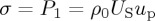). Figure 4a illustrates the determination of the Hugoniot parameters using the slope of the target Rayleigh line ρ₀U_S. In addition, the Hugoniot parameters can also be calibrated by σ_x, V_P and the known EOS of the standard flyer material.

Figure 6.

(a) Stress gauge trace from gabbro at a V_P of 826 m s⁻¹. (b) The beat waveform showing amplitude fluctuations of the moving surface. (c) The expanded time base revealing the individual beat cycles. (d) The velocity trace from the spectrogram calculated by Fourier transform. (Online version in colour.)

In the reverse impact tests, the beat waveform in figure 6b shows amplitude fluctuations of the moving surface, and the expanded time base in figure 6c reveals the individual beat cycles. The surface of the target moves through a distance equal to one-half of the laser wavelength (1550 nm), and a measured period of 5.1 ns corresponds to a free surface velocity u_fs of 152 m s⁻¹. Figure 6d shows the free surface velocity trace from the spectrogram calculated by Fourier transform and the numbers (2, 4, 6 and 8) denote the shock states for the determination of the shock release behaviour. The Hugoniot state can be determined from the slope of the target Rayleigh line ρ₀(C₀ + Su_p), and the particle velocity u_p (approx. u_p = 0.5u_fs, as described by Duvall & Fowles [56]) and impact velocity V_P, as schematically shown in figure 5b.

While each of the methods should lead to the same Hugoniot data, it should be mentioned that the method has advantages and disadvantages depending on precisely the measurement and the material being investigated. The PDV system has excellent time resolution, but monitors only the material surface. Manganin gauges provide in-material results, and simultaneously with the use of more than one gauge to determine the opportunity to measure shock velocity and/or shock wave attenuation. In addition, the cost of the gauges is significantly less than that of the PDV system. However, it has also been demonstrated that for certain rock-like materials the noise associated with gauge traces is sufficient to warrant using a reverse impact configuration and the PDV system to obtain more reliable results [57]. Shock behaviour plotted in P–u_p space is preferred in this study because either P or u_p is directly measured in experiments. The other parameters in U_S–u_pand P–V graphs can be computed by classical shock equations.

Figure 7a presents the measured Hugoniot states for these rock materials in shock velocity–particle velocity (U_S–u_p) space. The EOS relations between U_S and u_p are linearly fitted U_S = 5.485 + 1.038u_p and U_S = 2.62 + 3.319u_p for gabbro and marble, respectively. Although U_S–u_p results of gabbro [26,31] and marble [58] were also presented in the literature, the values of C₀ and S and the bulk wave speed of rocks were not given. For gabbro, the fitted values of C₀ and S are 6.409 (0.286 < u_p< 0.60) [26], 5.965 (0.286 < u_p< 0.60) [31], and 0.215 [26], 0.411 [31], respectively. For marble, the fitted values of C₀ and S are 2.57 and 2.50 (0.115 < u_p< 0.958) [58], respectively. It was found that, for gabbro, the constant C₀ that is the same as the bulk wave speed of 5.485 km s⁻¹ and S = 1.038 are similar to the values for ceramics [45]. By contrast, marble appears to have the value of C₀ (2.62 km s⁻¹), significantly below the calculated bulk wave speed (4.25 km s⁻¹) in table 2. It perhaps indicates a significant loss of strength or a phase transition of calcite (Carrara marble has 98% calcite composition) at a pressure of approximately 1.2 GPa [27,45]. Moreover, marble indicates a much higher value of S, which probably reveals the subsequent yield or transition attested by the third wave during shock compression [45].

Figure 7.

Measured Hugoniot states in: (a) the shock velocity--particle velocity (U_S–u_p) space, (b) the stress–particle velocity (P–u_p) space (the elastic response is calculated by P = ρ₀C_Lu_p) and (c) the pressure-specific volume (P–V) space. (Online version in colour.)

Above the HEL, the material loses much of its shear strength, though generally this is without the two-wave behaviours generally seen in shocked metals, for example. Attempts have been made to measure the shear strength and to then determine the deviation from elastic behaviour and infer an HEL [33]. In addition, the following relationship between the HEL and spall strength (σ_spall) with the Griffith criterion is given by [59]

4.1

Spall strength and Poisson's ratio v of most rock materials are 0.01–0.13 GPa [60] and 0.10–0.35 [61], respectively, suggesting that the HEL values are in the range of 0.11–7.51 GPa.

The Hugoniot data derived from the stress gauge and PDV records are shown in figure 7b. The Hugoniots lie slightly below the theoretical elastic lines (). The Hugoniot of gabbro in the pressure–particle velocity (P–u_p) plane is well fitted by a linear function . The data for marble fit better with a second-order polynomial relation , which might be induced by the phase transition of calcite [27,45].

The specific volumes of rocks are derived using the Hugoniot equations (equation (2.2), conservation of energy), and the Hugoniot curves in pressure (P) and relative specific volume (V₁/V₀) are shown in figure 7c. Unlike the gabbro that is the linear relation, , the marble has a nonlinear P–V curve, , and does not converge towards any value in this stress range. In addition, at a pressure close to 10 GPa, the gabbro is compressed to approximately 90% of its initial volume, which is less than 84% of that observed in the marble. As proposed by Eakins & Thadhani [41] the complete collapse of porosities occurs at high pressure. The phase transition of calcite is at a pressure of 1.2 GPa [27,45], which is lower than the shock pressure in this study. Thus, the primary reasons are that the gabbro with large well-formed interlocking crystals has less porosity (here, the porosity is defined by microcracks along crystals and scattered intergranular pores) than the marble and the phase transition of calcite in marble.

5. Conclusion

Plate impact experiments were conducted to determine the Hugoniot EOS of fine-grained marble and coarse-grained gabbro at high pressures up to 12 GPa. Manganin stress gauges and a PDV system were used for the measurement of stress, shock particle velocity and free surface velocity. Two compression testing methods conducted to obtain Hugoniot curves provided satisfactory results. The shock velocity–particle velocity (U_S–u_p) data of two rocks were fitted by straight lines in this pressure range. The Hugoniot curves in the plane of both the pressure–particle velocity (P–u_p) and pressure–relative specific volume (P − V₁/V₀) are well fitted by a linear function, and a polynomial function for gabbro and marble, respectively.

Authors' contributions

Q.B.Z. made substantial contributions to the conception, acquisition of data, analysis and interpretation of data; and drafted the article for important intellectual content. C.H.B. made substantial contributions to the conception and design. J.Z. gave final approval of the version to be published.

Competing interests

We have no competing interests.

Funding

This work is supported by the Swiss National Science Foundation (grant no. 200020_129757).

References

- 1.Boehler R. 2000. High-pressure experiments and the phase diagram of lower mantle and core materials. Rev. Geophys. 38, 221–245. ( 10.1029/1998RG000053) [DOI] [Google Scholar]
- 2.Short NM. 1966. Effects of shock pressures from a nuclear explosion on mechanical and optical properties of granodiorite. J. Geophys. Res. 71, 1195–1215. ( 10.1029/JZ071i004p01195) [DOI] [Google Scholar]
- 3.Trunin RF. 1994. Shock compressibility of condensed materials in strong shock waves generated by underground nuclear explosions. Phys. Usp. 37, 1123–1145. ( 10.1070/PU1994v037n11ABEH000055) [DOI] [Google Scholar]
- 4.Ross M, Graboske HC, Nellis WJ. 1981. Equation of state experiments and theory relevant to planetary modelling. Phil. Trans. R. Soc. Lond. A 303, 303–313. ( 10.1098/rsta.1981.0204) [DOI] [Google Scholar]
- 5.Kenkmann T, Poelchau MH, Wulf G. 2014. Structural geology of impact craters. J. Struct. Geol. 62, 156–182. ( 10.1016/j.jsg.2014.01.015) [DOI] [Google Scholar]
- 6.Anderson OL. 1995. Equations of state of solids for geophysics and ceramic science. Oxford, UK: Oxford University Press. [Google Scholar]
- 7.Ahrens TJ. 1993. Equation of state. In High-pressure shock compression of solids (eds Asay JR, Shahinpoor M), pp. 75–113. New York, NY: Springer. [Google Scholar]
- 8.Marsh SP. 1980. LASL shock Hungoniot data. Berkeley, CA: University of California Press. [Google Scholar]
- 9.McQueen RG, Marsh SP, Fritz JN. 1967. Hugoniot equation of state of twelve rocks. J. Geophys. Res. 72, 4999–5036. ( 10.1029/JZ072i020p04999) [DOI] [Google Scholar]
- 10.Trunin R. 1998. Shock compression of condensed materials. Cambridge, UK: Cambridge University Press. [Google Scholar]
- 11.Trunin R, Simakov G, Podurets M, Moiseyev B, Popov L. 1971. Dynamic compressibility of quartz and quartzite at high pressure. Izv. Acad. Sci. USSR Phys. Solid Earth 1, 13–20. [Google Scholar]
- 12.Trunin RF. 2001. Shock compression of condensed materials (laboratory studies). Phys. Usp. 44, 371–396. ( 10.1070/PU2001v044n04ABEH000919) [DOI] [Google Scholar]
- 13.Stöffler D. 1982. Terrestrial impact breccias. In Lunar breccias and soils and their meteoritic analogs (eds Taylor GJ, Wilkening LL), pp. 139–146. LPI Technical Report 82-02. Houston, TX: Lunar and Planetary Institute; See http://articles.adsabs.harvard.edu/full/1982lbsm.work.139S/0000146.000.html. [Google Scholar]
- 14.Stöffler D. 1982. 1.3 Density of minerals and rocks under shock compression. In Landolt-Börnstein—group V geophysics 1A (subvolume A) (eds Angenheister G.), pp. 120–126. Berlin, Germany: Springer. [Google Scholar]
- 15.Grady DE, Kipp ME. 1979. The micromechanics of impact fracture of rock. Int. J. Rock Mech. Min. Sci. Geomech. Abstr. 16, 293–302. ( 10.1016/0148-9062(79)90240-7) [DOI] [Google Scholar]
- 16.Kanel GI, Bless SJ, Rajendran AM. 2000. Behavior of brittle materials under dynamic loading. Technical report no. ADA386439. Institute for Advanced Technology, The University of Texas at Austin, Austin, TX, USA. See http://www.dtic.mil/cgi-bin/GetTRDoc?AD=ADA386439.
- 17.Rossmanith HP, Daehnke A, Nasmillner REK, Kouzniak N, Ohtsu M, Uenishi K. 1997. Fracture mechanics applications to drilling and blasting. Fatig. Fract. Eng. Mater. Struct. 20, 1617–1636. ( 10.1111/j.1460-2695.1997.tb01515.x) [DOI] [Google Scholar]
- 18.Zhao J, et al. 1999. Rock dynamics research related to cavern development for ammunition storage. Tunn. Undergr. Sp. Tech. 14, 513–526. ( 10.1016/S0886-7798(00)00013-4) [DOI] [Google Scholar]
- 19.Willmott GR, Proud WG. 2007. The shock Hugoniot of Tuffisitic Kimberlite Breccia. Int. J. Rock Mech. Min. 44, 228–237. ( 10.1016/j.ijrmms.2006.07.006) [DOI] [Google Scholar]
- 20.Braithwaite C. 2009. High strain rate properties of geological materials. Cambridge, UK: University of Cambridge. [Google Scholar]
- 21.Zhang QB. 2014. Mechanical behaviour of rock materials under dynamic loading. Lausanne, Switzerland: École Polytechnique Fédérale de Lausanne. [Google Scholar]
- 22.Kirk S. 2014. Shock compression and dynamic fragmentation of geological materials. Cambridge, UK: University of Cambridge. [Google Scholar]
- 23.Lysne PC. 1970. A comparison of calculated and measured low-stress Hugoniots and release adiabats of dry and water-saturated tuff. J. Geophys. Res. 75, 4375–4386. ( 10.1029/JB075i023p04375) [DOI] [Google Scholar]
- 24.Ahrens TJ, Gregson VG Jr. 1964. Shock compression of crustal rocks: data for quartz, calcite, and plagioclase rocks. J. Geophys. Res. 69, 4839–4874: ( 10.1029/JZ069i022p04839) [DOI] [Google Scholar]
- 25.Larson DB, Anderson GD. 1980. Plane shock wave studies of Westerly granite and Nugget sandstone. Int. J. Rock Mech. Min. Sci. Geomech. Abstr. 17, 357–363. ( 10.1016/0148-9062(80)90519-7) [DOI] [Google Scholar]
- 26.Boslough MB, Ahrens TJ. 1985. Shock wave properties of anorthosite and gabbro. J. Geophys. Res. 90, 7814–7820. ( 10.1029/JB090iB09p07814) [DOI] [Google Scholar]
- 27.Davies FW, Smith EA. 1994. High pressure equation of state investigation of rocks. Contract no. ADA284761. Albuquerque, NM: Ktech Corp. [Google Scholar]
- 28.Nakazawa S, Watanabe S, Kato M, Iijima Y, Kobayashi T, Sekine T. 1997. Hugoniot equation of state of basalt. Planet. Space Sci. 45, 1489–1492. ( 10.1016/S0032-0633(97)00070-6) [DOI] [Google Scholar]
- 29.Sekine T, Kobayashi T, Nishio M, Takahashi E. 2008. Shock equation of state of basalt. Earth Planets Space 60, 999–1003. ( 10.1186/BF03352857) [DOI] [Google Scholar]
- 30.Shang JL, Shen LT, Zhao J. 2003. Hugoniot equation of state of the Bukit Timah granite. Int. J. Rock Mech. Min. 37, 705–713. ( 10.1016/S1365-1609(00)00002-2) [DOI] [Google Scholar]
- 31.Millett JCF, Tsembelis K, Bourne NK. 2000. Longitudinal and lateral stress measurements in shock-loaded gabbro and granite. J. Appl. Phys. 87, 3678–3682. ( 10.1063/1.372399) [DOI] [Google Scholar]
- 32.Lomov IN, Hiltl M, Vorobiev OY, Glenn LA. 2001. Dynamic behavior of berea sandstone for dry and water-saturated conditions. Int. J. Impact Eng. 26, 465–474. ( 10.1016/S0734-743X(01)00097-5) [DOI] [Google Scholar]
- 33.Tsembelis K, Proud WG, Field JE. 2002. The principal Hugoniot and dynamic strength of Dolerite under shock compression. AIP Conf. Proc. 620, 1385–1388. ( 10.1063/1.1483797) [DOI] [Google Scholar]
- 34.Johnson D, Chapman DJ, Tsembelis K, Proud WG. 2007. The response of dry limestone to shock-loading. AIP Conf. Proc. 995, 1387–1390. ( 10.1063/1.2832984) [DOI] [Google Scholar]
- 35.Yuan F, Prakash V. 2013. Plate impact experiments to investigate shock-induced inelasticity in Westerly granite. Int. J. Rock Mech. Min. 60, 277–287. ( 10.1016/j.ijrmms.2012.12.024) [DOI] [Google Scholar]
- 36.Zhernokletov MV. 2006. Methods and devices for producing intense shock loads. In Material properties under intensive dynamic loading. Shock wave and high pressure phenomena (eds Zhernokletov MV, Glushak BL), pp. 33–71. Berlin, Germany: Springer. [Google Scholar]
- 37.Bourne N. 2013. Materials in mechanical extremes: fundamentals and applications. Cambridge, UK: Cambridge University Press. [Google Scholar]
- 38.Ahrens TJ. 1987. 6. Shock wave techniques for geophysics and planetary physics. In Methods in experimental physics, vol. 24, part A (eds Charles GS, Thomas LH), pp. 185–235. New York, NY: Academic Press. [Google Scholar]
- 39.Lexow B, Wickert M, Thoma K, Schäfer F, Poelchau M, Kenkmann T. 2013. The extra-large light-gas gun of the Fraunhofer EMI: applications for impact cratering research. Meteorit. Planet. Sci. 48, 3–7. ( 10.1111/j.1945-5100.2012.01427.x) [DOI] [Google Scholar]
- 40.Ramesh KT. 2008. High rates and impact experiments. In Springer handbook of experimental solid mechanics (ed. Sharpe WN.), pp. 929–960. New York, NY: Springer. [Google Scholar]
- 41.Eakins DE, Thadhani NN. 2009. Shock compression of reactive powder mixtures. Int. Mater. Rev. 54, 181–213. ( 10.1179/174328009X461050) [DOI] [Google Scholar]
- 42.Meyers MA. 1994. Dynamic behavior of materials. New York, NY: John Wiley & Sons, Inc. [Google Scholar]
- 43.Bourne NK, Millett JCF, Gray GT III. 2009. On the shock compression of polycrystalline metals. J. Mater. Sci. 44, 3319–3343. ( 10.1007/s10853-009-3394-y) [DOI] [Google Scholar]
- 44.Field JE, Walley SM, Proud WG, Goldrein HT, Siviour CR. 2004. Review of experimental techniques for high rate deformation and shock studies. Int. J. Impact Eng. 30, 725–775. ( 10.1016/j.ijimpeng.2004.03.005) [DOI] [Google Scholar]
- 45.Grady DE. 1998. Shock-wave compression of brittle solids. Mech. Mater. 29, 181–203. ( 10.1016/S0167-6636(98)00015-5) [DOI] [Google Scholar]
- 46.Hiermaier S. 2008. Structures under crash and impact: continuum mechanics, discretization and experimental characterization. Berlin, Germany: Springer Science & Business Media. [Google Scholar]
- 47.Chapman DJ. 2009. Shock compression of porous materials and diagnostic development. Cambridge, UK: University of Cambridge. [Google Scholar]
- 48.Bourne NK, Rosenberg Z, Johnson DJ, Field JE, Timbs AE, Flaxman RP. 1995. Design and construction of the UK plate impact facility. Meas. Sci. Technol. 6, 1462 ( 10.1088/0957-0233/6/10/005) [DOI] [Google Scholar]
- 49.Strand OT, Goosman DR, Martinez C, Whitworth TL, Kuhlow WW. 2006. Compact system for high-speed velocimetry using heterodyne techniques. Rev. Sci. Instrum. 77, 083108 ( 10.1063/1.2336749) [DOI] [Google Scholar]
- 50.Lea LJ, Jardine AP. 2016. Application of photon Doppler velocimetry to direct impact Hopkinson pressure bars. Rev. Sci. Instrum. 87, 023101 ( 10.1063/1.4940935) [DOI] [PubMed] [Google Scholar]
- 51.Al'tshuler LV, Kormer SB, Brazhnik MI, Vladimirov LA, Speranskaya MP, Funtikov AI. 1960. The isentropic compressibility of aluminium, copper, lead, and iron at high pressures. [English translation.] Sov. Phys. JETP. 11, 761–775. See http://www.jetp.ac.ru/cgi-bin/dn/e_011_04_0766.pdf. [Google Scholar]
- 52.Zhang QB. 2016. Shear strength and Hugoniot elastic limit (HEL) of rock materials under shock loading. In Rock dynamics: from research to engineering (eds Li HB, Li JC, Zhang QB, Zhao J), pp. 227–232. Boca Raton, FL: CRC Press. [Google Scholar]
- 53.Murri WJ, Grady DE, Mahrer KD. 1975. Equation of state of rocks. SRI Project PYU-1883. Stanford Research Institute, Menlo Park, CA, USA. [Google Scholar]
- 54.Millett JCF, Tsembelis K, Bourne NK, Field JE. 2000. The shock Hugoniot of two igneous rocks. AIP Conf. Proc. 505, 1247–1250. ( 10.1063/1.1303687) [DOI] [Google Scholar]
- 55.Rosenberg Z, Yaziv D, Partom Y. 1980. Calibration of foil-like manganin gauges in planar shock wave experiments. J. Appl. Phys. 51, 3702–3705. ( 10.1063/1.328155) [DOI] [Google Scholar]
- 56.Duvall G, Fowles G. 1963. Shock waves. In High pressure physics and chemistry, vol. 2 (ed. Bradley RS.), pp. 209–291. New York, NY: Academic Press. [Google Scholar]
- 57.Guest AR, Braithwaite CH, Proud WG, Field JE.. 2007. The shock Hugoniot properties of geological materials and relationship to static properties. AIP Conf. Proc. 995, 1379–1382. ( 10.1063/1.2832981) [DOI] [Google Scholar]
- 58.Furnish M. 1994. Dynamic properties of Indiana, Fort Knox and Utah test range limestones and Danby marble over the stress range 1 to 20 GPa. Albuquerque, NM: Sandia National Labs. [Google Scholar]
- 59.Rosenberg Z. 1993. On the relation between the Hugoniot elastic limit and the yield strength of brittle materials. J. Appl. Phys. 74, 752–753. ( 10.1063/1.355247) [DOI] [Google Scholar]
- 60.Grady DE, Hollenbach RE. 1979. Dynamic fracture strength of rock. Geophys. Res. Lett. 6, 5 ( 10.1029/GL006i002p00073) [DOI] [Google Scholar]
- 61.Gercek H. 2007. Poisson's ratio values for rocks. Int. J. Rock Mech. Min. Sci. 44, 1–13. ( 10.1016/j.ijrmms.2006.04.011) [DOI] [Google Scholar]