Metrics for rapid quality control in RNA structure probing experiments

Abstract

Motivation: The diverse functionalities of RNA can be attributed to its capacity to form complex and varied structures. The recent proliferation of new structure probing techniques coupled with high-throughput sequencing has helped RNA studies expand in both scope and depth. Despite differences in techniques, most experiments face similar challenges in reproducibility due to the stochastic nature of chemical probing and sequencing. As these protocols expand to transcriptome-wide studies, quality control becomes a more daunting task. General and efficient methodologies are needed to quantify variability and quality in the wide range of current and emerging structure probing experiments.

Results: We develop metrics to rapidly and quantitatively evaluate data quality from structure probing experiments, demonstrating their efficacy on both small synthetic libraries and transcriptome-wide datasets. We use a signal-to-noise ratio concept to evaluate replicate agreement, which has the capacity to identify high-quality data. We also consider and compare two methods to assess variability inherent in probing experiments, which we then utilize to evaluate the coverage adjustments needed to meet desired quality. The developed metrics and tools will be useful in summarizing large-scale datasets and will help standardize quality control in the field.

Availability and Implementation: The data and methods used in this article are freely available at: http://bme.ucdavis.edu/aviranlab/SPEQC_software.

Contact: saviran@ucdavis.edu

Supplementary information: Supplementary data are available at Bioinformatics online.

1 Introduction

RNA plays an integral role in many biological processes, spanning an enormous range of functionalities (Sharp, 2009), whose root often lies in structure. Discerning structure is thus of paramount importance, but it remains a challenging task, as traditional methods such as crystallography are time consuming whereas computational approaches struggle to correctly predict it by sequence alone. The recent advent of affordable and efficient high-throughput structure probing experiments has helped address these deficiencies (Cheng et al., 2015; Ding et al., 2014; Hector et al., 2014; Kertesz et al., 2010; Kielpinski and Vinther, 2014; Lucks et al., 2011; Mortimer et al., 2012; Poulsen et al., 2015; Rouskin et al., 2014; Sager et al., 2015; Seetin et al., 2014; Smola et al., 2015; Spitale et al., 2014, 2015; Talkish et al., 2014; Underwood et al, 2010; Wan et al., 2013; Watters et al., 2016). Furthermore, their outputs can be used to constrain structure prediction algorithms and improve prediction accuracy (Deigan et al., 2009; Lorenz et al., 2015, 2016; Markham and Zuker, 2008; Reuter and Mathews, 2010) or utilized in other applications (Kutchko et al., 2015, Lavender et al., 2015). Probing experiments use reagents, such as SHAPE and DMS, which modify RNA residues in a structure-dependent manner (Weeks, 2010). Modifications are detected via reverse transcription, which terminates at modified sites. Noise due to random terminations is measured in a control assay. Modification and control measurements are then combined to yield a final reactivity score: residues with high reactivities are more likely to be unstructured, while low reactivities are suggestive of pairing interactions (Sükösd et al., 2013).

The newest generation of experiments utilizes high-throughput sequencing to detect modifications, allowing for unprecedented multiplexing capabilities. Focus is now shifting towards in vivo and transcriptome-wide studies, leading to a breadth of new insights (Mortimer et al., 2014). While these developments are exciting, they face significant challenges in standardizing data due to differences in chemistries, protocols and analysis strategies. For example, most techniques detect modifications as reverse transcriptase (RT) terminations, but others induce mutations at modified sites (Smola et al., 2015). Despite these differences, reactivity calculation reduces to a comparison of detection rates between modified and control channels, giving rise to a unified approach for evaluating and optimizing data analysis (Shih et al., in revision). But even if methods are standardized, tools are needed to evaluate data quality obtained by each of these experiments (Aviran and Pachter, 2014).

The problem of quality control can be addressed in rudimentary ways when examining a few transcripts, through visual inspection or simple statistical tests. As the field moves towards large-scale genome-wide and in vivo experiments, evaluating quality of datasets or individual transcripts becomes increasingly difficult. Examination of these data must consider issues such as non-uniform coverage, priming biases, increased transcript lengths, large number of transcripts and increased number of replicates. Similar to challenges faced in early stages of microarrays and RNA-Seq (Bolstad et al., 2003; Ritchie et al., 2015), a convenient and standardized method for quality control must be developed.

We present broadly applicable methods to analyze and to improve reproducibility of structural data. At the core of our approach is a generalizable metric that we introduce, which quantifies agreement among replicates. We validate and characterize it on SHAPE-Seq data obtained in highly controlled in vitro conditions, featuring multiple replicates and very deep coverage across eight well-characterized RNAs (Loughrey et al., 2014). Our validation then reveals a quality threshold to be used with this metric, thereby facilitating simple and rapid preliminary quality screenings. We also address situations where multiple replicates are not available and present methods for quality control, which quantify technical variability in experiments. Finally, we explore additional applications of our approach, such as analysis of large-scale in vivo datasets, reproducibility verification for differential analysis and experiment design. Our tools are designed with simplicity in mind, making quality assessment accessible to experimentalists. Our work represents the first generation of broadly applicable quality control methods in structure probing experiments, a necessary step in the maturation of this field.

2 Methods

We extracted SHAPE-Seq counts for three replicates of eight RNAs with lengths ranging from 74 to 338 nt and for a single replicate of TPP riboswitch in absence and presence of ligand, all probed in vitro. Three processed SHAPE-Seq replicates of HIV RRE before and after Rev-RRE complex formation in vitro were provided by Yun Bai. We also processed raw reads into counts from two replicates of yeast and mouse transcriptome-wide in vivo Mod-Seq and icSHAPE experiments, respectively. See Supplementary Information for details.

2.1 Reactivity reconstruction

Extracted counts tally the number of modifications detected at each residue k in the modified (plus) and control (minus) channels. In SHAPE-Seq and similar assays, counts represent RT stop or termination events, obtained by identifying all sequenced cDNAs whose 3′ ends map to one residue downstream of k. SHAPE-Seq profiles were obtained by initializing RT at a single priming site at each transcript’s 3′ end, resulting in cDNAs spanning sequences between priming and stop sites. Such targeted priming allowed us to recover the local coverage, which is the sequencing depth at a residue, defined as the number of reads that either stop at or pass through said residue (see Supplementary Fig. S1). We denote stop counts in plus and minus channels by X_k and Y_k, respectively, and local coverages in said channels by C_k+and C_k-, respectively. We then converted counts into two stop rates, X_k/C_k+ and Y_k/C_k-, to normalize them for variation in local coverages among residues and channels.

Transcriptome-wide profiles were obtained from random primer extension (RPE) experiments coupled with single-end reads to identify stop sites only. In such protocols, absence of mate-pair reads precludes recovery of local coverages (Supplementary Fig. S1). Instead, for each transcript, we used its average number of mapped reads per residue.

Plus channel stop counts reflect a combined effect of modification and natural RT termination, or noise. To measure the degree of modification at residue k, we defined its reactivity, β_k, as its probability of being modified. To estimate the noise component in the plus channel counts, we introduced an auxiliary parameter, γ_k, as the probability that RT stops at residue k due to factors others than modification. Our goal was to estimate the β_k’s from sequencing data.

We used a model-based maximum-likelihood (ML) approach to estimation, previously developed for similar data (Aviran et al., 2011a). The ML estimate (MLE) of γ_k was directly recovered from minus channel data as the ratio of the kth stop count to the kth local coverage count, Y_k/C_k-. A simple and intuitive way to account for noise in plus channel is to estimate β_k as the difference of stop rates between channels (Eq. 1):

$${\widehat{\beta }}_k=\mathrm{ }\frac{X_k}{C_{k+}}-\mathrm{ }{\widehat{\mathrm{ }\gamma }}_k;\mathrm{ }{\widehat{\mathrm{ }\gamma }}_k=\mathrm{ }\frac{Y_k}{C_{k-}}$$

We chose this estimate for its simplicity and because its outputs closely matched those of β_k’s MLE, which takes a more complex form (Aviran et al., 2011b; Shih et al., in revision). Note that while β_k is constrained by definition to lie in the unit interval, there is no guarantee that ${\widehat{\beta }}_k\ge 0$, as it is a difference of two terms from independent channels. Indeed, such data inconsistencies between channels arise in practice, and we employed a standard remedy of setting negatives to 0. Notably, ML estimation yields the same principle (Aviran et al., 2011b).

Differences in experimental conditions and transcript properties result in varying degrees of modification (i.e. signal power) among reactivity profiles. The extent to which a transcript was modified, or its modification rate, was computed by summing the ${\widehat{\beta }}_k$’s. To bridge these differences, we normalized each profile with the commonly used 2–8% strategy (Sloma and Mathews, 2015; Low and Weeks, 2010). This step amounts to scaling by a constant and it is necessary for placing all measurements on common scale prior to any comparative or joint analysis. Normalized values would then be placed both below and above 1.

For transcriptome-wide data, reactivities were similarly reconstructed, with the difference that stop rates were evaluated with respect to transcript coverages. See Supplementary Information for further details.

2.2 SNR calculation

SNR per residue k was calculated as the ratio of its reactivity’s sample mean to sample standard deviation (Equation 2):

$${\mathrm{S}\mathrm{N}\mathrm{R}}_k=\frac{{\mathrm{\mu }}_k}{{\mathrm{\sigma }}_k}.$$

It is undefined when standard deviation is zero (reactivities are equal). SNR can be summarized over a stretch of residues or entire transcript in various ways, e.g. mean, boxplot or pie chart. To reduce the sensitivity of the mean to outliers and improve its robustness, we clipped all values above 35 and set them to 35 (see Supplementary Information for details).

2.3 Bootstrap analysis

Bootstrap resampling was performed using the sample function in R. Resampling of both start and stop counts could be done for paired-end reads. However, SHAPE-Seq experiments used single-primer extension with fixed start site. Hence, only resampling of stop counts was required. Local coverage was determined by summing stop counts at or downstream of a residue. More detail and performance evaluation are included in Supplementary Information.

2.4 Variance estimates

A closed-form expression was derived to estimate variances of reactivity estimates as alternative to bootstrap. Assuming (i) binomial distribution; (ii) statistical independence of terminations in plus and minus channels; and (iii) fixed local coverage; variance can be estimated as (Equation 3):

$$\widehat{Var}\left({\widehat{\beta }}_k\right)=\frac{\widehat{Var}(X_k)}{C_{k+}^2}+\frac{\widehat{Var}(Y_k)}{C_{k-}^2}=\frac{\left({\widehat{\beta }}_k+{\widehat{\gamma }}_k\left(1-{\widehat{\beta }}_k\right)\right)\left(1-{\widehat{\beta }}_k-{\widehat{\gamma }}_k\left(1-{\widehat{\beta }}_k\right)\right)}{ C_{k+}}+\frac{{\widehat{\gamma }}_k\left(1-{\widehat{\gamma }}_k\right)}{C_{k-}}.$$

Its derivation and the derivation for reactivity calculated as a ratio are described in Supplementary Information.

2.5 Coverage quality index (CQI)

We developed a scoring strategy—coverage quality index (CQI)—to assess coverage adjustments required to meet user-specified quality criteria. Specifically, we asked for an acceptable range of variation (ε_k) around the mean reactivity and a significance level, which represents the likelihood that reactivity estimates from experiments with predicted coverage level would deviate from current estimates within that allowed range. Range of variation is defined as a percentage error around the reactivity. Given the percentage error and z-value corresponding to significance level, we estimated the variance of reactivities, under the assumption that they are Gaussian random variable, as (Equation 4):

$${\widehat{Var}}_{\mathrm{N}\mathrm{o}\mathrm{r}\mathrm{m}\mathrm{a}\mathrm{l}}\left({\widehat{\beta }}_k\right)=\mathrm{ }{\left(\frac{{\epsilon }_k\mathrm{*}\mathrm{ }{\widehat{\beta }}_k}{z_{\mathrm{v}\mathrm{a}\mathrm{l}\mathrm{u}\mathrm{e}}}\right)}^2.$$

This variance is then substituted into Equation (3) to solve for desired local coverage, C_k+, keeping ${\widehat{\beta }}_k$ and ${\widehat{\mathrm{ }\mathrm{\gamma }}}_k$ fixed. CQI is calculated as the ratio of desired coverage to current coverage. The indices for low, medium and high reactivities were summarized as the 95th percentile for each category and presented together as what we call ‘95% CQI’. See Supplementary Information for more details and for validation.

3 Results

Differences in experimental conditions result in inevitable variability between replicates. For experiments that probe a few RNAs, visual/manual inspection of replicate data makes quality control relatively straightforward (Aviran and Pachter, 2014). However, the recent emergence of transcriptome-wide experiments presents challenges in rapidly screening a multitude of long transcripts or regions within them for strong or weak replicate agreement. Here, we propose a quantitative and broadly applicable approach to automatically assess this, which will be useful for researchers as they evaluate small or large datasets. We first introduce the basic concept and validate its efficacy using a small high-quality dataset obtained in well-controlled conditions. This not only confirms the method’s indicative power but also results in simple guidelines for rapid quality assessment. With a simple approach at hand, we strive to broaden its scope through its application to additional problems and biological scenarios. These include reproducibility assessment in the absence of replicates, experiment design for improved reproducibility, analysis of transcriptome-wide data and reproducibility measurement in differential analysis situations. Some of these instances also triggered us to develop novel adjoining methods, which we describe below.

3.1 Using signal-to-noise ratio to assess reproducibility

At the core of our approach is a concept co-opted from signal processing, the signal-to-noise ratio (SNR), as a simple and informative metric of reproducibility, which quantifies disagreement between replicates irrespective of the underlying sources of variation. Here, we calculate SNR as ratio of a reactivity’s mean to its standard deviation (see Section 2), as commonly done in image analysis (Bushberg et al., 2012).

We use a SHAPE-Seq dataset (Loughrey et al., 2014) to demonstrate our metric’s capacity to discern high-quality data, as this set encompasses numerous well-characterized and highly structured RNAs, featuring three replicates for each RNA (see Section 2). Even though replicates were generated under the same conditions, differences arise in a similar manner to those observed in biological replicates, though in this case RNAs were transcribed in vitro. This allows us to validate our method in a simple setting before applying it to more complex situations.

To establish the diagnostic capacity of SNR, we look at agreement among pairs of replicates. We generate reactivity profiles for each replicate using a previously derived estimation method coupled with a widely used normalization strategy (see Section 2). Three replicates of eight RNAs give rise to 24 pairwise comparisons. To qualitatively demonstrate how SNR measures replicate concurrence, consider two pairs that contrast in their level of agreement: the hepC IRES domain features consistent overlaps, while cyclic di-GMP has several regions of discrepancies (Fig. 1A–B). SNR captures these differences well, as can be seen from box plots of residue SNR distributions per transcript. Such differences are clearly observed when represented as the mean value of a transcript (Fig. 1A, insets). Thus, summary statistics such as mean SNR may be useful in assessing agreement over regions of RNA.

Fig. 1.

Validation and characterization of SNR as a measure of replicate agreement in a small synthetic library. (A) Two RNAs that display strong or poor replicate agreement (continuous and dashed lines). Insets show box plots of their residue SNR distributions, with corresponding mean SNRs marked by horizontal (blue) lines as well as annotated on SNR axes. The box plots reveal the presence of high residue SNR values, leading to high mean SNR, for hepC IRES, while for cdGMP, residue SNR is concentrated at low values, resulting in low mean SNR. (B) Scatter plot representations of pairwise replicate agreement for each RNA. (C) Relationship of mean SNR and Pearson correlation for 24 pairwise replicate comparisons. Line marks high-quality threshold of 5. (D) Correlation of mean SNR with the following controllable experimental parameters (top to bottom): minus channel coverage rate, plus channel coverage rate and modification rate. Each panel features 24 dots corresponding to 24 SHAPE-Seq profiles. SNR for each profile was estimated from bootstrap simulations of stop counts (Color version of this figure is available at Bioinformatics online.)

Next, we quantitatively evaluate how well mean SNR captures replicate agreement for all 24 pairwise comparisons. We examine mean SNR’s relationship with a common pairwise evaluation statistic—Pearson correlation. We find that both provide reliable evaluations of agreement, as replicate pairs with strong SNR also display high correlation coefficients (Fig. 1C). Notably, a sharp increase in correlation coefficients toward 1 is associated with mean SNR values ranging from 3 to 5, with 5 marking a plateauing of such step-like relationship. This observation further simplifies the use of mean SNR, as it allows for rapid preliminary screening: replicates with SNR greater than 5 can be confidently classified as high quality. It is also worth noting that values between 3 and 5 may also signify good replicate agreement, although with lower confidence. For transcripts that fall in this ambiguous range, we recommend further examination via boxplot analysis of residue SNR scores, to reveal where the bulk of the distribution lies (Fig. 1A, insets). Finally, SNR confers another advantage: it accommodates an arbitrary number of replicates, a feature that traditional correlation tests do not have unless they involve complex statistical considerations.

3.2 Reproducibility assessment in the absence of replicates

Numerous factors other than biological variation exert their effect on probing measurements. For example, chemical reactions and detections are inherently stochastic, and repeated library preparation followed by sequencing results in technical variability. In the absence of multiple replicates, it is still possible to assess such form of variability. Here, we propose two methods, one data-driven and the other model-based.

Non-parametric approach. A simple and well-established approach is to leverage resampling methods in order to synthesize ‘fake’ replicates in lieu of real ones. An appealing feature is their capacity to generate large numbers of replicates, which is infeasible in the lab. This has the potential to improve mean and variance estimation precision. It is thus advantageous to use SNR in such setting, as traditional reproducibility metrics or visual inspection become prohibitive when replicate numbers exceed 2 or 3. By readily accommodating a multitude of replicates, SNR allows us to reap the benefits of both powerful computers and large-sample statistics. We mimic replicates through bootstrap simulations, synthesizing multiple datasets from the original one rather than relying on any model assumptions. We repeatedly resample the distribution of SHAPE-Seq counts a hundred times and reconstruct reactivities as described above, keeping coverage at original level (approximately 8000 reads per residue on average). See Section 2 and Supplementary Information for implementation details.

Parametric approach. It is important to acknowledge potential limitations of bootstrap. The computational resources required in resampling can be limiting, especially as complexity and scale of experiments increase. Bootstrapping SHAPE-Seq data is straightforward because of the small number of RNAs and the usage of a single primer. Thus, all reads start at the same site and one merely resamples stop sites. In contrast, paired-end reads originating from RPE experiments warrant greatly increased computational effort to account for both start and stop sites, amounting to quadratic growth in the size of count distributions from which one resamples. This is exacerbated in transcriptome-wide studies, as transcript numbers, lengths and the sequencing volume render resampling computationally demanding, if not infeasible.

To address such issues, we derive a formula to estimate variance in reactivities given stop counts and local coverage at a residue (see Section 2). We treat the probability of a read as binomially distributed and then express the standard deviation of the simplified MLE described in Section 2. To validate the efficacy of such formula-based estimate, we compare it to the bootstrap-based one (see Supplementary Information for details). Overall, we find that formula calculations yield results similar to those generated by laborious simulations.

3.3 Application to experiment design

In experiment design, one seeks to identify key controllable determinants to data variability (Aviran and Pachter, 2014). We accomplish this by comparing mean SNR per transcript with controllable factors from each probing experiment: plus and minus channel per-residue coverage, total coverage per channel, ratio of channel coverages, and modification rate (see Section 2). Interestingly, we find that plus channel coverage shows a stronger correlation (r = 0.74) than minus channel coverage (r = 0.4) (Fig. 1D). In contrast, modification rate (Fig. 1D) and ratio of coverage between plus and minus channels (not shown) have no correlation with SNR strength. Notably, we see similar trends for experimental replicates, with moderate correlation between SNR and coverage levels (not shown). The agreement between experimental and simulated results not only validates our method, but more importantly highlights how SNR elucidates key determinants of quality.

3.3.1 Data-informed coverage adjustment

Increasing coverage is an obvious route to improving quality; yet, it is costly. One may want to first evaluate the extent of necessary adjustments—a non-trivial task. Here, we address this need by developing a new metric: coverage quality index (CQI). Given desired reproducibility, CQI measures if current local coverage levels are sufficient to maintain them and, if not, approximates how much more coverage is needed.

We first frame reproducibility in terms of individual constraints on admissible degrees of fluctuation at each residue. For realistic modeling, we turn to SHAPE-Seq data, where we observe differing variabilities. We find that the relationship between a reactivity’s mean and its standard deviation is linear on a log scale, such that standard deviation increases at nearly the same rate as the mean (Supplementary Fig. S2).

Based on this, we assume that a reactivity’s variability is proportional to itself. A target coefficient of proportion (ε_k) is to be set by the user. For example, if a reactivity is 0.5, ε = 20% would result in values within (0.4, 0.6). We use ε_k and a user-defined significance level (α) to calculate the corresponding variance (σ²_k) of reactivities, under the assumption that fluctuation magnitudes are Gaussian (Fig. 2; see Section 2). For example, if we use α = 95%, then σ²_k would be the variance at which Gaussian samples fall within the set interval with 95% confidence. We then insert σ²_k into our variance estimation formula, which allows us to solve for the local coverage (C_k*) required for maintaining the target variability (Equation 4; see Section 2). CQI is the ratio of desired coverage to original coverage (C_k*/C_k). Residues with CQI scores less than 1 are considered adequately covered, while those higher than 1 may warrant higher coverage to ensure desired quality. CQIs that exceed 1 can also provide an estimate of the fold-increase in coverage required.

Fig. 2.

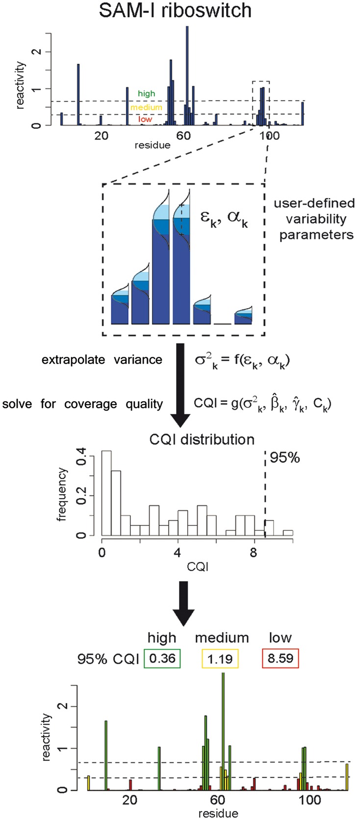
Workflow for CQI calculations. Top bar graph shows data for SAM-I riboswitch. Dashed lines separate reactivities into low/medium/high categories. Zoomed inset of reactivities highlights two user-defined parameters: significance level, illustrated by the shaded area under the Gaussian curves placed on top of each reactivity bar, and desired fluctuation intensity, depicted by the dashed error bar. Vertical arrow and formulas below the inset represent core calculations for each residue: extrapolation of desired variance and its subsequent use in conjunction with reactivity and noise estimates to determine desired local coverage and ultimately the ratio of desired to existing coverages (CQI). Lower two panels show the resulting CQI residue distribution and its summarization for each category into a single number by taking the 95% percentile of CQIs in that category (vertical dashed line). Reactivities and CQIs in bottom panel are color-coded by categories (low/medium/high) (Color version of this figure is available at Bioinformatics online.)

An example of CQI calculation is shown for the SAM-I riboswitch (Fig. 2). As CQI is generated for each residue, we summarize indices for an entire transcript by taking the 95th percentile of CQIs (95% CQI) (vertical dashed line). This conservative metric identifies the residue requiring the most coverage to ensure desired quality after trimming potential outliers (see Supplementary Information for details). Since low probability events require large sample sizes for precise estimation, lower reactivities demand higher coverage to meet desired quality criteria and can push 95% CQI to a high value. But small reactivities remain small even in the face of large fluctuations, and such imprecision may not be a major concern. To provide a comprehensive yet structurally relevant view of coverage, we apply the same approach to three ranges: low, medium and high. In our example, the SAM-I riboswitch has adequate coverage to limit variability to 10% in high and medium reactivities, but not in low ones (Fig. 2). 95% CQIs for each transcript and reactivity category correlate well with their corresponding bootstrap-based mean SNRs, where low 95% CQIs correlate with high mean SNRs (Supplementary Fig. S3). This is consistent with our findings that coverage and mean SNR are correlated (Fig. 1D).

For the target variabilities we tested, we find that all high reactivities and most medium ones in our data are adequately covered (Supplementary Fig. S3), as well as a majority of low reactivities. To test whether CQI is a good estimator of the coverage necessary to confine variability, we simulate predicted coverage adjustments via bootstrap (see Supplementary Information for details). We find that CQI is an accurate predictor of necessary coverage adjustment; it appropriately limits variability in 85% of our simulations, with better success in high reactivities (94%) than low reactivities (71%) (Supplementary Table F1). The dependence of success rates on reactivity magnitude is consistent with our formula’s tendency to be less accurate at low coverage. By utilizing variance estimates from both bootstrapping and formula, we validate CQI as another informative quality control and experiment design metric.

3.4 Application to other biological scenarios

3.4.1 Transcriptome profiling in vivo

Having demonstrated our method on a small synthetic library, we now examine quality characteristics when data are obtained with more advanced protocols and in a cellular environment. Such data display significantly higher complexities in terms of spectrum of coverages, lengths and structural properties. A Mod-Seq experiment (Talkish et al., 2014) used DMS to probe yeast cells via RPE coupled with single-end reads to map stop sites. To showcase SNR’s application to identifying regions of high or poor quality within a long transcript, we consider a well-covered 18S rRNA from this dataset. We calculate rolling mean SNR for center-aligned windows of 51 nt (Fig. 3A). Since DMS probes only A and C and since zero reactivities frequently arise in both replicates, the rolling mean summarizes only a subset of residues in a window. For robust inference, we limit attention to means reporting a relatively high fraction of residues (dark bars) and identify two regions whose good/poor quality stands out. We find that this quality disparity could be explained by local stop counts statistics (see inset), which are less controllable with RPE. Interestingly, the poor-quality region has very low counts in all four channels, hinting at a possible systematic bias. Similar cause-and-effect relationship can be seen at the 3′ end, as commonly observed in stop-based data. This analysis demonstrates SNR’s utility in picking up variations within transcripts and in exploring technical biases.

Fig. 3.

Transcriptome profiling in vivo. (A) Mod-Seq data: bars represent center-aligned rolling mean of SNR over windows of 51 nt. Color gradient indicates fraction of residues in a window for which SNR is defined. Windows of considerably high or low quality, where SNR is defined for high fraction of residues (dark bars), are marked with arrows pointing to window range in inset. Inset shows mean of stop counts in both channels of two replicates. (B–C) icSHAPE data: (B) Pearson correlation vs. mean SNR. Marker shapes denote Gini index of residue SNRs for a transcript. Colors indicate plus coverage rate averaged over replicates. Inset highlights a more pronounced trend in well-covered transcripts (labeled blue in B) and their fit to a theoretical relationship. Also shown is a similar trend in pairwise SHAPE-Seq comparisons. (C) Tukey boxplots of residue SNRs for well-covered transcripts (labeled blue in B) with mean SNR > 5. A continuous line connects their mean SNRs. Markers on top indicate their Gini index (as labeled in B) and color gradient indicates Pearson correlation. Ensembl gene IDs are given, where * stands for ENSMUSG000000. In panels A and C, background is divided into three quality zones: green for good (>5), yellow for ambiguous (3–5), red for poor (<3) (Color version of this figure is available at Bioinformatics online.)

Furthermore, differences in counts may be more dramatic when gleaned across a transcriptome. Since Mod-Seq contains robust information for a small portion of cellular RNAs, we analyze a more comprehensive icSHAPE dataset (Spitale et al., 2015) of mouse stem cells in vivo. Here, large variation in transcript abundances, manifested as coverage differences, is an additional factor modulating quality. An SNR-Pearson plot reveals a trend reminiscent of SHAPE-Seq’s step-like behavior, albeit with much greater scatter (Fig. 3B). While this scatter may be expected due to noisy conditions, we find that much of it is attributed to transcripts with low coverage and to those in which a small proportion of residues dominates the overall sum of residue SNRs (quantified by high Gini index, marked by ‘+’ in Fig. 3B). Indeed, when restricting analysis to well-covered transcripts, a clearer and tighter trend emerges, which closely matches SHAPE-Seq’s characteristics (Fig. 3B, inset). This suggests simple guidelines for identifying subsets of better precision and more robust information. Interestingly, both datasets are fit well by known theoretical relationship (see Supplementary Information). Such quantitative agreement between two vastly different datasets attests to the generality of SNR as a quality metric.

Since coverage re-emerges as major determinant of quality, we next screen for transcripts with mean SNR > 5 and plus coverage rate > 25. Boxplot analysis (Fig. 3C) shows that for most of them, SNR distributions substantially overlap medium (yellow) and high-quality (green) zones. With the exception of a few RNAs with borderline mean SNR, they display good correlation. This further validates mean SNR’s discriminative power in preliminary screening. We further find that most transcripts with poor correlation also have high Gini index (+ marks), suggesting simple quantitative tools for further refinement. Our analysis also highlights that challenging conditions might impact screening specificity, warranting careful analysis. It is worth noting that both datasets appear to be of poorer quality than SHAPE-Seq, possibly because of less favorable conditions, randomness in priming and less precise reactivity calculation due to missing coverage information when using single-end reads (see Section 2).

3.4.2 Reproducibility of differential signals

Thus far, we have defined reproducibility in a restricted sense as mean SNR > 5, but other experimental situations may justify other criteria. For example, Bai et al. (2014) used SHAPE-Seq to detect differences between protein-bound and protein-free states of HIV’s Rev-response element (RRE) in vitro. Reactivity changes observed in three replicates, each consisting of profiles before and after Rev-RRE complex formation, signified protein binding. In such differential analysis situations, we consider data as sufficiently reproducible if replicate agreement within conditions exceeds that of in-between conditions. This confirms that differential signals can be reliably estimated. To address this notion quantitatively, we analyze five SNR distributions: within conditions (two distributions, three replicates each) and between conditions (one distribution each for three replicates). Restricting analysis to binding sites (which consist a small fraction of the entire sequence), we find that within each condition, a greater fraction of residues shows strong agreement, whereas agreement degrades in between-conditions comparisons (Supplementary Fig. S4). This quantitatively validates that data are sufficiently reproducible. See Supplementary Information for an additional application to differential analysis of structural changes in a riboswitch.

4 Scope and constraints

Current techniques encompass diverse chemistries, modification detection methods, library preparation strategies (random/targeted priming, size selection), sequencing choices (single/paired-end reads) and analysis pipelines. This diversity presents challenges for proposed quality control methods, as they should bridge these differences to standardize assessment and facilitate comparative analysis.

Aside from its simplicity and computational ease, SNR is a versatile metric applicable directly to reactivities, irrespective of how they were reconstructed or of the specifics of the experiment and sequencing. Another advantage that renders SNR suitable for comparative analysis of datasets is that it accommodates an arbitrary number of replicates.

While SNR calculations may follow any reactivity reconstruction, for a given transcript, different reconstructions might result in different SNR values. Consistency in the informatics approach taken is thus imperative to quality comparisons across datasets. Due to a multitude of proposed analysis options (Shih et al., in revision), here we carried out all analyses using a single choice. We caution, however, that the dependency of SNR values on the analysis method may warrant recharacterizing the ‘high quality’ threshold for other choices. Note that we repeated the analysis in Figure 1C for another commonly used alternative (i.e. ratio of stop rates) and found that the general SNR-Pearson trend remains the same (see Supplementary Information). Also, in less controlled conditions, it may be beneficial to refine the threshold test by closely examining its outcomes. Accounting for additional metrics may also be informative.

Direct applicability to reactivities grants SNR its universality, yet it also results in ambiguity, particularly when zeros are concordantly observed across replicates. If capturing a structure signal, they are informative, but they could also be a manifestation of a fading signal (i.e. no counts). Importantly, coverage disparities within transcriptome-wide data make them more prone to this deficiency, which can be remedied by sensible integration of coverage information. Resolving such ambiguity may also improve data-directed structure inference (Deng et al., 2016).

Finally, while SNR reveals discordant measurements, it cannot resolve sources of variation. Possible sources include poor coverage, low sequencing or alignment quality, structure differences, biological/technical variability, high background and inefficient reactions. Even design choices, such as single-end reads or cDNA size selection, discard information that might then affect reproducibility. Because SNR measures a compound effect as well as lacks an underlying statistical model, it cannot determine, for example, if variation can be explained by changes in structure (up to a desired confidence level). Although the approach can be equipped with such model to facilitate hypothesis testing, this would compromise its simplicity, which we consider to be its most appealing property for practical purposes. Yet, in its present form, it may become useful as rapid pre-screen for differential analysis, based on the expectation that when differential effects are present, replicates would better agree within conditions than between conditions.

The two approaches we proposed for estimating SNR’s variance component differ in their generality. Bootstrap is straightforward to apply and requires no modeling assumptions. In contrast, the formula relies on simplifying assumptions and requires re-derivation to other reconstruction methods, e.g. when estimating reactivity as a ratio between plus and minus channel rates (see Supplementary Information). It also makes direct use of local coverage information. In its absence (e.g. when combining single-end sequencing with RPE), its accuracy might degrade. Note that these limitations carry over to CQI.

When deriving the formula, we also fixed the local coverage, although it is currently unclear how realistic this is, especially in transcriptome-wide setting, where coverage is not easily controllable. Loss of coverage may also adversely affect the formula’s performance, as we diverge from our assumption as well as deviate in the parameter estimates we use. Our tests using simulations indicate that while our formula performs well at high coverage, its robustness breaks down at low coverage (see Supplementary Information). Thus, we recommend using it in high coverage situations to save time while maintaining accuracy, whereas bootstrap may be favorable at low coverage, for its consistency and speed.

5 Discussion

As structure probing experiments increase in scope and complexity, analytical tools must keep pace to ensure efficient processing and reliable results. Whereas manual inspection of data was once sufficient, the extent of newer experiments precludes such approaches. The quantitative tools and framework we presented here are a first step in addressing this deficiency, providing quality controls that are standardized, generally applicable, automatable and scalable. We envision these tools to be used in design and analysis of new and emerging large-scale experiments.

To evaluate reproducibility, we used the concept of SNR as well as developed a new metric, CQI, which predicts coverage levels needed to achieve a desired fluctuation level. Both metrics involve straightforward calculations; yet they are informative at both the replicate and transcript levels. One favorable characteristic of SNR is its flexibility to handle multiple replicates, experimental or simulated. While it is a useful quantification at both the residue and whole-transcript levels, the mean SNR statistic has the advantage of distilling reproducibility information across any number of residues into a single number, allowing for rapid preliminary screening of large-scale datasets. More elaborate summarizations of residue SNR distributions or subsets thereof, such as boxplot and categorical chart analyses, may complement this approach as means of inspecting borderline outcomes, detecting regions of special interest, or accommodating alternative criteria for overall reproducibility.

CQI performs a similar task, aggregating coverage information across a transcript into three indices. This metric has similar advantages as SNR: it serves as rapid quantification with a clear quality threshold and is easily automated. It provides a preliminary estimate of the coverage increase necessary to limit variability and can be subsequently fine-tuned via resampling. Importantly, the variability we simulated does not encapsulate all sources of noise; thus, recommendations by CQI should be seen as a minimum recommended coverage increase rather than a fix-all solution. This metric builds off of our formula-based estimate, which explicitly links coverage to data variability. It thereby demonstrates the usefulness of this classical approach compared to modern resampling methods. The formula also has the added benefit of rapid estimation compared to bootstrap, though the latter may be more accurate at low coverage. Nonetheless, the tandem of bootstrap and formula provide a computational way to quantitatively evaluate data quality.

The data summarization we employed here is readily generalizable to other proposed quality measures (Smola et al., 2015; Talkish et al., 2014; Yang et al., 2002). One common strategy in microarrays is to report the ratio of signal to background (Yang et al., 2002). We derived a formula for this ratio’s variability (see Supplementary Information). While this may be a good way to evaluate enrichment, it did not perform as well as the mean SNR as summary statistic when correlated with coverage or modification rate (not shown). The ratio measure is also not as broadly applicable, as it is limited to single residues/transcripts.

The presented methods are relatively straightforward and by no means address all issues, but are a first step towards ensuring high-quality data. As the field continues to grow, effort must be spent on both pioneering new techniques as well as analysis and visualization tools (Choudhary et al., in revision). One plausible avenue for improvement is to combine RPE with paired-end sequencing for better consistency in recovering local coverage information. Our methods attempt to unify how researchers quality-control their data. We kept our work simple and accessible, to make its adoption as painless and fruitful as possible. We aim to establish a foundation for more sophisticated platforms, which will ultimately bridge differences among protocols and expedite the field’s maturation.

References

- Aviran S. et al. (2011a) Modeling and automation of sequencing-based characterization of RNA structure. Proc. Natl. Acad. Sci., 108, 11069–11074. [DOI] [PMC free article] [PubMed] [Google Scholar]
- Aviran S. et al. (2011b) RNA structure characterization from chemical mapping experiments. In: Proceedings of the 49th Annual Allerton Conference on Communication, Control, and Computing. Monticello, IL, pp. 1743–1750.
- Aviran S., Pachter L. (2014) Rational experiment design for sequencing-based RNA structure mapping. RNA, 20, 1864–1877. [DOI] [PMC free article] [PubMed] [Google Scholar]
- Bai Y. et al. (2014) RNA-guided assembly of Rev-RRE nuclear export complexes. Elife, 3, e03656. [DOI] [PMC free article] [PubMed] [Google Scholar]
- Bolstad B.M. et al. (2003) A comparison of normalization methods for high density oligonucleotide array data based on variance and bias. Bioinformatics, 19, 185–193. [DOI] [PubMed] [Google Scholar]
- Bushberg J.T. et al. (2012) The Essential Physics of Medical Imaging. Lippincott Williams & Wilkins, Philadelphia, Pennsylvania, USA. [Google Scholar]
- Cheng C.Y. et al. (2015) Consistent global structures of complex RNA states through multidimensional chemical mapping. Elife, 44, e07600. [DOI] [PMC free article] [PubMed] [Google Scholar]
- Deigan K.E. et al. (2009) Accurate SHAPE-directed RNA structure determination. Proc. Natl. Acad. Sci., 106, 97–102. [DOI] [PMC free article] [PubMed] [Google Scholar]
- Deng F. et al. (2016) Data-directed RNA secondary structure prediction using probabilistic modeling. RNA, 22, 1109–1119. [DOI] [PMC free article] [PubMed] [Google Scholar]
- Ding Y. et al. (2014) In vivo genome-wide profiling of RNA secondary structure reveals novel regulatory features. Nature, 505, 696–700. [DOI] [PubMed] [Google Scholar]
- Hector R.D. et al. (2014) Snapshots of pre-rRNA structural flexibility reveal eukaryotic 40S assembly dynamics at nucleotide resolution. Nucl. Acids. Res., 42, 12138–12154. [DOI] [PMC free article] [PubMed] [Google Scholar]
- Kertesz M. et al. (2010) Genome-wide measurement of RNA secondary structure in yeast. Nature, 467, 103–107. [DOI] [PMC free article] [PubMed] [Google Scholar]
- Kielpinski L.J., Vinther J. (2014) Massive parallel-sequencing-based hydroxyl radical probing of RNA accessibility. Nucl. Acids. Res., 42, e70.. [DOI] [PMC free article] [PubMed] [Google Scholar]
- Kutchko K.M. et al. (2015) Multiple conformations are a conserved and regulatory feature of the RB1 5′ UTR. RNA, 21, 1274–1285. [DOI] [PMC free article] [PubMed] [Google Scholar]
- Lavender C.A. et al. (2015) Model-free RNA sequence and structure alignment informed by SHAPE probing reveals a conserved alternative secondary structure for 16S rRNA. PLoS Comput. Biol., 11, e1004126. [DOI] [PMC free article] [PubMed] [Google Scholar]
- Lorenz R. et al. (2015) SHAPE directed RNA folding. Bioinformatics, 32, 145–147. [DOI] [PMC free article] [PubMed] [Google Scholar]
- Lorenz R. et al. (2016) Predicting RNA secondary structures from sequence and probing data. Methods, 103, 86–98. [DOI] [PubMed] [Google Scholar]
- Loughrey D. et al. (2014) SHAPE-Seq 2.0: systematic optimization and extension of high-throughput chemical probing of RNA secondary structure with next generation sequencing. Nucl. Acids. Res., 42, e165. [DOI] [PMC free article] [PubMed] [Google Scholar]
- Low J.T., Weeks K.M. (2010) SHAPE-directed RNA secondary structure prediction. Methods, 52, 150–158. [DOI] [PMC free article] [PubMed] [Google Scholar]
- Lucks J.B. et al. (2011) Multiplexed RNA structure characterization with selective 2′-hydroxyl acylation analyzed by primer extension sequencing (SHAPE-Seq). Proc. Natl. Acad. Sci., 108, 11063–11068., [DOI] [PMC free article] [PubMed] [Google Scholar]
- Markham N.R., Zuker M. (2008) UNAFold: software for nucleic acid folding and hybridization. Methods Mol. Biol., 453, 3–31. [DOI] [PubMed] [Google Scholar]
- Mortimer S.A. et al. (2012) SHAPE-Seq: high throughput RNA structure analysis. Curr. Protoc. Chem. Biol., 4, 275–297. [DOI] [PubMed] [Google Scholar]
- Mortimer S.A. et al. (2014) Insights into RNA structure and function from genome-wide studies. Nat. Rev. Genet., 15, 469–479. [DOI] [PubMed] [Google Scholar]
- Poulsen L.D. et al. (2015) SHAPE Selection (SHAPES) enrich for RNA structure signal in SHAPE sequencing-based probing data. RNA, 21, 1042–1052. [DOI] [PMC free article] [PubMed] [Google Scholar]
- Reuter J.S., Mathews D.H. (2010) RNAstructure: software for RNA secondary structure prediction and analysis. BMC Bioinformatics, 11, 129.. [DOI] [PMC free article] [PubMed] [Google Scholar]
- Ritchie M.E. et al. (2015) limma powers differential expression analyses for RNA-sequencing and microarray studies. Nucleic Acids Res., 43, e47. [DOI] [PMC free article] [PubMed] [Google Scholar]
- Rouskin S. et al. (2014) Genome-wide probing of RNA structure reveals active unfolding of mRNA structures in vivo. Nature, 505, 701–705. [DOI] [PMC free article] [PubMed] [Google Scholar]
- Sager J.G. et al. (2015) Global analysis of the RNA-protein interaction and secondary structure landscapes of the Arabidopsis nucleus. Mol. Cell, 57, 376–388., [DOI] [PMC free article] [PubMed] [Google Scholar]
- Seetin M.G. et al. (2014) Massively parallel RNA chemical mapping with a reduced bias MAP-seq protocol. Methods Mol. Biol., 1086, 95–117. [DOI] [PubMed] [Google Scholar]
- Sharp P.A. (2009) The centrality of RNA. Cell, 136, 577–580. [DOI] [PubMed] [Google Scholar]
- Sloma M.F., Mathews D.H. (2015) Improving RNA secondary structure prediction with structure mapping data. Methods Enzymol., 553, 91–114. [DOI] [PubMed] [Google Scholar]
- Smola M.J. et al. (2015) Selective 2′-hydroxyl acylation analyzed by primer extension and mutational profiling (SHAPE-MaP) for direct, versatile and accurate RNA structure analysis. Nat. Protoc., 10, 1643–1669. [DOI] [PMC free article] [PubMed] [Google Scholar]
- Spitale R.C. et al. (2014) RNA structural analysis by evolving SHAPE chemistry. Wiley Interdiscip. Rev. RNA, 5, 867–881. [DOI] [PMC free article] [PubMed] [Google Scholar]
- Spitale R.C. et al. (2015) Structural imprints in vivo decode RNA regulatory mechanisms. Nature, 519, 486–490. [DOI] [PMC free article] [PubMed] [Google Scholar]
- Sükösd Z. et al. (2013) Evaluating the accuracy of SHAPE-directed RNA secondary structure predictions. Nucleic Acids Res., 41, 2807–2816. [DOI] [PMC free article] [PubMed] [Google Scholar]
- Talkish J. et al. (2014) Mod-seq: high-throughput sequencing for chemical probing of RNA structure. RNA, 20, 713–720. [DOI] [PMC free article] [PubMed] [Google Scholar]
- Underwood J.G. et al. (2010) FragSeq: transcriptome-wide RNA structure probing using high-throughput sequencing. Nat. Methods, 7, 995–1001. [DOI] [PMC free article] [PubMed] [Google Scholar]
- Wan Y. et al. (2013) Genome-wide mapping of RNA structure using nuclease digestion and high-throughput sequencing. Nat. Protoc., 8, 849–869. [DOI] [PubMed] [Google Scholar]
- Watters K.E. et al. (2016) Simultaneous characterization of cellular RNA structure and function with in-cell SHAPE-Seq. Nucleic Acids Res., 44, e12. [DOI] [PMC free article] [PubMed] [Google Scholar]
- Weeks K.M. (2010) Advances in RNA structure analysis by chemical probing. Curr. Opin. Struct. Biol., 20, 295–304. [DOI] [PMC free article] [PubMed] [Google Scholar]
- Yang Y.H. et al. (2002) Normalization for cDNA microarray data: a robust composite method addressing single and multiple slide systematic variation. Nucleic Acids Res., 30, e15. [DOI] [PMC free article] [PubMed] [Google Scholar]
Associated Data
This section collects any data citations, data availability statements, or supplementary materials included in this article.